Waste haven effect: unwrapping the impact of environmental regulation

(1)

HAL Id: halshs-01339837

https://halshs.archives-ouvertes.fr/halshs-01339837

Submitted on 30 Jun 2016

HAL is a multi-disciplinary open access

archive for the deposit and dissemination of sci-entific research documents, whether they are

pub-L’archive ouverte pluridisciplinaire HAL, est destinée au dépôt et à la diffusion de documents scientifiques de niveau recherche, publiés ou non,

Waste haven effect: unwrapping the impact of

environmental regulation

Thais Nuñez-Rocha

To cite this version:

Thais Nuñez-Rocha. Waste haven effect: unwrapping the impact of environmental regulation. 2016. �halshs-01339837�

(2)

Documents de Travail du

Centre d’Economie de la Sorbonne

Waste haven effect: unwrapping the impact

of environmental regulation

Thais N

UNEZ-

R

OCHA

(3)

Waste haven effect: unwrapping the impact

of environmental regulation

Thais Nunez-Rocha

May, 2016

Abstract

A new branch of the literature on international trade and environment suggests that developing countries are becoming waste havens for their developed counterparts, due to environmental regulation differences with trade partners. This paper analyses the effectiveness of the Basel Convention formalisation in the European Union (EU-WSR), by studying the impact of the EU-WSR on hazardous waste trade, first on the less developed EU countries, and then on regions of developing countries. It does so, by means of a gravity model framework applied to a panel data-set. Results show that there is no enough evidence to call for waste haven effect in the less developed EU countries, with both aggregated and disaggregated measures of environmental regula-tions, but increasing institution efficiency differences could lead to increasing imports of waste. In the regional analysis, there is no evidence of the efficacy of the EU-WSR. These findings provide insights into the efficacy of European engagements on waste trade, indicating that there is no simple answer as to its effect.

Keywords: Hazardous waste, waste haven effect, international trade,

international environmental agreements, difference-in-differences, log-linear and ppml gravity model.

(4)

1 Introduction

The relationship between trade and environment has raised a great deal of interest among economists, despite the fact that simultaneity of the two poses serious empirical challenges, because when trade increases the environmental damage tends to increase as well. Addi-tionally, even if the simultaneity issue is addressed, whether trade has a positive or negative impact on the environment has not emerged consensual answer yet.

A first theoretical puzzle is to assess the environmental impact of trade. Such impact can be decomposed into three main components: the scale effect, due to the increasing magnitude of trade, the technique effect, i.e. the impact that new technologies may have on pollution intensity, and the composition effect, caused by a change in the type of production in place (Grossman and Krueger [1991]). This paper focuses on the latter effect, by controlling for scale and technique effect. Following Copeland and Taylor [2003], the composition effect is broken down into its two driving forces: factor of endowments and environmental regulation differences.

The second puzzle is the challenge that estimating this effect empirically can represent. In general, empirical research concentrates in cross-sectional studies, observing environ-mental impact of trade through emissions as in Cole and Elliott [2003] Frankel and Rose [2005], Managi et al. [2009] and Baghdadi et al. [2013] or industry location as channel of attraction of possible pollution haven effect (?, Dean et al. [2009]). The literature is much less extensive when it comes to estimate the hazardous waste trade, despite the natural intuition that some negative effect is likely to be found. Exporting hazardous waste to countries with lenient environmental regulation saves the cost from industry relocation, Jug and Mirza [2005] support the fact that environmental regulation has an impact in trade flows. From a policy point of view, this is unfortunate, because waste trade harms the country environmental quality, not even leaving much of an investment, as is the case of the pollution haven effect.

According to Misra and Pandey [2005] hazardous waste, when mishandling in any envi-ronmental media may have both short- and long-term effects on both human and environ-mental systems. Improper treatment, storage, and disposal of hazardous waste can result in contaminant during possible exposures, and potential adverse health and environmental impacts. In the case of this study, even if the flow of hazardous waste shipped from de-veloped to developing countries represents less then 3% of total trade, irresponsible waste management practices can create hazardous conditions and considerable risks to human health. In general, any toxic component can cause severe health consequences, even death if taken by humans in sufficiently large amounts.

(5)

concern because even in small doses, can cause adverse health impacts. Some anecdotal evidence show that irresponsible management of heavy metals included in some devises as in this analyses ”Waste and scrap of primary cells, primary batteries and electric articles” are highly toxic even in low doses, specially to those repeatedly exposed to them. Those substances can have effects to the nervous systems, kidneys and other organs. The effects of particular concern are those from lead and mercury on the development of the nervous system in children, other chemicals including some brominated flame retardants can build up in human bodies from repeated exposures and for some there is evidence of long term effects including brain development and the whole immune system, many chemicals in

electronic devises are also environmental persistent.1 There are illegal and legal waste

shipments (Bernard [2011]), in the framework of this study due to data-availability only legal shipments are studied.

Among the studies that directly address waste trade, several are based on cross-sectional data and treat the phenomenon as a pollution haven effect, either including capital abun-dance (Baggs [2009]), or including the analysis of environmental regulation differences be-tween countries (Kellenberg [2012]), also these two papers concentrate in all waste and not only hazardous waste. In order to control for endogenous simultaneity between trade and environment, panel-data offer a better setting; this is in line with Kellenberg and Levin-son [2014], although their analysis is not extensive in terms of disentangling the groups of countries or regions being more (or less) affected by this trade, and the composition ef-fect, including the differences in environmental regulation between countries, is not directly investigated.

This article is most closely related to Kellenberg [2012]. Kellenberg [2012] uses cross-sectional data-set from the 2003-2004 and also directly asses the environmental regulation difference issue. He uses the Global Competitiveness Report, as a proxy of the environ-mental regulation, this index is based on a report having answers of company executives ranking the enforcement of environmental regulations at country-level. The findings of this paper are that environmental regulation across countries are an important determinant of waste trade in developing countries.

This analysis differs from Kellenberg [2012] in several respects, some are methodological and other are conceptual, but all of them make more accurate results for policy recommen-dation.

First, in the methodological part the contribution is that this analysis uses panel data-set in order to disentangle the possible simultaneity of the formalisation, which could be a result of countries selecting themselves into the formalisation depending on their volume of waste trade (Baier and Bergstrand [2007]). Also, the environmental regulation index used

1

(6)

is a composite index, this index has multiple dimensions in order to asses different features of the environmental regulation (Brunel and Levinson [2013]). It contains information about three complementary indicators as in ?, but in this case, those that are relevant

for waste trade are taken. The advantage of using such index is that it captures the

solidity of institutions, the actual state of the environmental outcome and the presence of environmental trade barriers. Relevance of institutions to trade has been proven important in Rodriguez and Rodrik [2001] and to pollution in Barrett and Graddy [2000] and in Candau and Dienesch [2015], this is the first study to include institution quality in waste trade analysis. These contributions are discussed in detail in the methodology and results sections.

Second, in the conceptual differences, here only hazardous waste are analyzed due to their polluting potential, and also because non-hazardous waste can also be recycled and used as raw materials. The work of Kellenberg and Levinson [2014] is also on a panel data frame-work but frame-works with all types of waste, and uses only two groups of countries developed and developing. In this work goes one step forward and explore the waste haven effect both in the less developed EU countries and in developing countries; this separation on different country-group, allows to give more precise conclusions on the determinants in force when waste trade is studied. Finally, developing countries are also separated into regions to see

closer the effect in each region.2

The remainder of this paper is organized as follows. Section 2 introduces the international context on waste trade and some stylized facts. Section 3 describes the empirical strategy. The results are presented in section 4. Section 5 concludes.

2 International context on waste

In the late eighties, claims made by developing countries attracted the attention of the International community. Those complaints were mainly addressed by African developing countries, claiming that waste was being illegally disposed in their territories. Their efforts resulted in the Basel Convention on waste trade, which entered into force in 1992. In its early days, the instrument implemented by the convention was the Prior Informed Consent (PIC), a formal mechanism allowing a country to send waste shipments to another country, conditional on the ’prior consent’ of the corresponding importing authority.

Some years later, developing countries claimed that waste trade had in fact increased over time (Kellenberg [2012]). This situation lead to the implementation of the Basel Ban Amendment in 1995. The Ban Amendment is intended to clearly prohibit shipments

2

(7)

of hazardous waste from developed to developing countries. Yet, because of the lack of

sufficient ratifying members, such instrument is still not in force. The effect of these

two instruments, in case of the Basel Convention, have shown no effect (Kellenberg and Levinson [2014]).

However, all the European Union (EU) members signed the Basel Convention and com-mitted to the Ban Amendment. To formalise this commitment, it had then to be written in the official journal of the EU, whence an EU regulation on shipments of waste was

cre-ated (EU-WSR).3 The formalisation of the Basel Convention in the EU passed in 2006

and it entered into force in 2007. It includes the Ban Amendment, despite the fact that the latter is not in force up to date. Even if European countries were to engage into not sending hazardous waste to developing countries, no legal binding procedure nor enforcing authority exist to settle potential cases of no compliance.

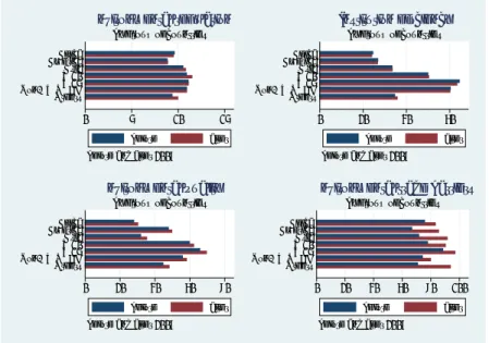
Being restricted to send waste to developing countries, the former and richer EU countries

(the EU-154) could be tempted to change their waste trading partners to their neighbors,

the new arrived and specially less developed countries (EU-105), which also have laxer

environmental regulations (See Figure 1).

2.1 Stylized facts

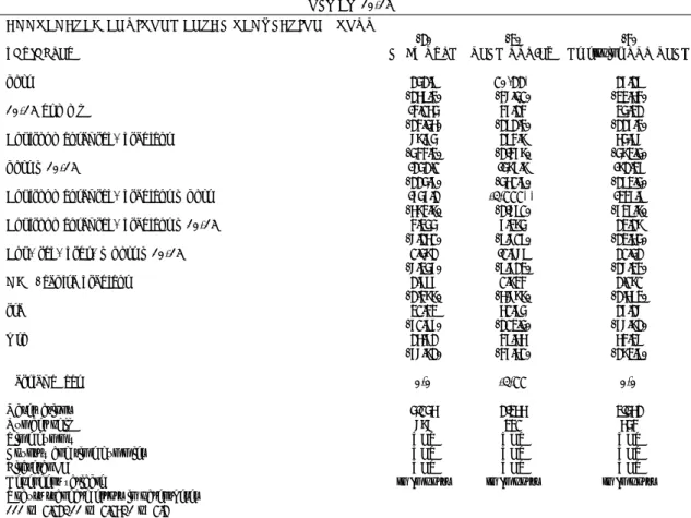
To see if increased trade was due to EU-WSR, I estimate first a simple difference regression; results are shown in Table 4 and 5 in appendix. The difference-in-difference estimation is not appropriate to disentangle the effect of environmental regulation as a determinant of waste trade. In order to include differences in environmental regulation and to control for time variant and invariant determinants of trade, these estimations are set up in a gravity model. Nevertheless, is interesting to have a first glance of the effect of this formalisation, the magnitude of the trade in each group of country and also how results change once adding all the controls.

Table 4 shows EU-10 waste imports coming from the EU-15 before and after the EU-WSR; this is the treatment group. As control group, the waste exports of the EU-15 to three groups of countries are considered: all countries of the world except the EU-10, the OECD non-EU and developing or non-OECD countries. Results vary in magnitude depending on

3

Council Regulation. No 1013/2006 of European parliament and of the council of 14 June 2006 on shipments of waste. It will be in force from, 12:1-98, 2007.

4

EU-15=Austria, Belgium, Denmark, France, Finland, Germany, Greece, Ireland, Italy Luxembourg, Netherlands, Portugal, Spain, Suede, United Kingdom

5_{EU-10=Cyprus, Czech Republic, Estonia, Hungary, Latvia, Lithuania, Malta and Poland. Bulgaria}

(8)

the group, but in all cases there is an increase in trade, although results are not significant in the difference-in-differences estimator.

In the regional analysis, the treatment groups are the African, Asian and American devel-oping countries whose waste imports are coming from the EU. As control groups, I consider their imports coming from non-EU OECD countries. All of them are studied before and after EU-WSR. Table 5 shows the results. A decrease in waste trade is observed in the African and American regions, although the results lose significance in the difference-in-differences estimator. In the case of Asia, the waste trade increases, but results are not significant.

3 Empirical strategy

3.1 Data

The key point in evaluating the effectiveness of the EU-WSR is to correctly define hazardous waste. To select the appropriate products, I referred to the definition of hazardous waste contained in the text of the Basel Convention ”A substance in order to be defined as hazardous waste, it must both be listed and possess a characteristic such as being explosive, flammable, toxic, or corrosive. Also, a product could enter in this category if it is defined as or considered to be a hazardous waste under the laws of either the exporting country,

the importing country, or any of the countries of transit”.6

The data-set used here is a matching process of these two sources of information: the COMTRADE data-set and the Basel Convention data-set, in time period 2003-2010. Due to the PIC the Basel Convention has information about the shipments of waste of countries reported to the importing authority, with the 6-digit HS codes a matching process was done of the shipments in the Basel Convention registers and the COMTRADE data-set. The advantage of such combination is that the number of observations is almost doubled, taking into account possibly mislabeling or irregular shipments.

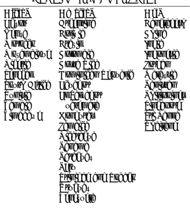
The type of products selected are those that have disposable waste in their description and/or in their name. Such definition includes industrial waste, municipal waste, waste oils, pharmaceutical waste, organic solvents waste, hydraulic fluids waste, brake fluids and anti freeze fluids waste, chemical products waste, primary cells waste, metal scrap, primary batteries and electric articles waste. For a full list of the products with their 6-digit harmonized system (HS) codes, refer to Table 6 in the appendix.

6_{This study concentrates only on hazardous waste, the broader definition of waste includes also non}

(9)

3.2 Variables

As explanatory variables, in order to represent the period (post)t after the EU-WSR and

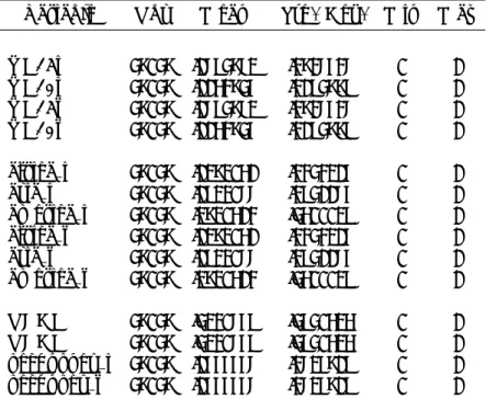
the country-group, a set of dummies is used. The country-groups are listed in Table 1. Moreover, following Kellenberg [2012], a measure of differences in costs is also constructed it helps to control for a matter of specialisation in some countries, due differences in costs rather than in environmental regulation within countries.

Variable Obs Mean Std. Dev. Min Max

UE15i 48048 .1794872 .3837637 0 1 UE10i 48048 .1153846 .3194889 0 1 UE15j 48048 .1794872 .3837637 0 1 UE10j 48048 .1153846 .3194889 0 1 africa i 48048 .1282051 .3343216 0 1 asia i 48048 .1923077 .3941176 0 1 america i 48048 .2820513 .4500029 0 1 africa j 48048 .1282051 .3343216 0 1 asia j 48048 .1923077 .3941176 0 1 america j 48048 .2820513 .4500029 0 1 OCDE 48048 .4230769 .4940525 0 1 OCDEP 48048 .4230769 .4940525 0 1 oecdnoneu i 48048 .1666667 .3726819 0 1 oecdnoeu j 48048 .1666667 .3726819 0 1

Table 1: Explained and explanatory variables

The dependent variable is the aggregated waste trade. It has been constructed using total weight imported, aggregated from the 6-digit HS, for the specific products that are subject to the definition of waste mentioned above. Those countries that do not trade certain products for the entire period under study are excluded from the main analysis. Even then, the quantity of zeros in the dependent variable is important.

Imports weight rather than value is used because it makes more sense from an environ-mental point of view (Kellenberg [2012]) and because, waste being not a regular product, the direction of the payment is not well established. Inside the products considered, there could be some of them that are exported to extract some material e.g. electronic devises, others could be exported just to disposal at lower costs either labor costs or environmental costs, for this reason there is not clear way to know if the value is the payment of importer country or exporter country.

(10)

3.3 Environmental regulation gradient

Studying hazardous waste imports derives its relevance from the polluting potential of such products. This is particularly true in developing countries, since countries who do not possess the installed capacity of producing products which ensue those waste products or by-products, improbably could manage their treatment or disposal in an environmentally

friendly way (Briggs [2003]).7 If a phenomenon of specialisation is emerging, it should be

captured by the costs gradient.

Furthermore, if a waste haven effect exists, developing countries environment and health outcomes could be affected not only by lax environmental regulations in loco, but also by stricter environmental regulations with trading partner countries. Measuring the difference in environmental regulation between countries helps identifying this channel, specifically in the case of waste imports, that cannot be considered as an importing ”good”, but rather as an environment-harming ”bad”. 0 5 10 15 Others Non-EU OECDEU 15 EU 10Asia AmericaAfrica

before and after 2007

by group of countries Environmental regulation before after 0 20 40 60 Others Non-EU OECDEU 15 EU 10Asia AmericaAfrica

by group of countries Institution efficiency before after 0 20 40 60 80 Others Non-EU OECDEU 15 EU 10Asia AmericaAfrica

by group of countries Environmental quality before after 0 20 40 60 80 100 Others Non-EU OECDEU 15 EU 10Asia AmericaAfrica

by group of countries Environmental trade barriers

before after

Figure 1: Environmental regulation components

The claims made by developing countries about the increased imports of hazardous waste after the enforcement of the Basel Convention pointed to the fact that institutions could

7

”Scope of the Chemicals and Waste Subprogramme” (UNEP and Harmful Sub-stances at a glance Division of Technology, Industry and Economics United Na-tions Environment Programme (UNEP) International Environment House. June 2010), http://www.unep.org/chemicalsandwaste/About/tabid/258/Default.aspx.

(11)

be corrupted. This fact could have lead to increased waste imports or maintained trends in this trade, as underlined by Kellenberg and Levinson [2014].

According to Ben Kheder and Zugravu [2012] and Brunel and Levinson [2013] a composed index of environmental regulation is necessary to measure the multidimensional features of the matter and to capture fundamental aspects such as the institutional efficiency, environ-mental outcomes and environenviron-mental trade barriers. The environenviron-mental regulation variable is estimated as an aggregated variable composed of these three indexes; estimations of these three complementary variables are also conducted in a disaggregated form in order to account for their individual effect. Further explanation about each variable is to be found in the appendix.

The environmental regulation gradient (ERG) ERGijt= (Ejt− Eit)/[(Ejt+ Eit)/2] that

captures the differences between countries, is constructed following Kellenberg [2012]. The gradient will increase as the differences in environmental regulation within a couple of countries trading waste increases, either because one country makes his regulation stricter or because the other makes it looser. The construction of the environmental regulation gra-dient, the normalisation of the three proxy variables and the estimation of the aggregated gradient are detailed in the Appendix A5 .

3.4 Model specification

In 2006, the EU parliament approved a regulation intended to ban shipments of hazardous waste to developing countries EU-WSR. This regulation is a formalisation of the Basel Convention and of its related Ban Amendment on hazardous waste. Using this information, I construct an indicator variable for bilateral trading pairs where exporting countries are the EU-15 and importing countries are EU-10; this dummy variable is coupled with a period variable, which distinguishes periods before and after 2007, the year in which the regulation entered into force. Finally, the interaction between these two variables and the ERG is considered.

To this difference-in-differences specification is joined gravity model of trade as the workhorse in estimating the effect of policy-based bilateral agreements on bilateral trade flows (Head and Mayer [2014]) and following the most recent developments of the gravity specification (Baier and Bergstrand [2007], Santos Silva [2011]).

An important issue in the estimation of the effects of a policy aimed at changing trade patterns is that potential self-selection of country pairs into more or less trading of the targeted products generates endogeneity bias in the estimates.

(12)

In order to deal with this several techniques are adopted; first, to avoid endogeneity bias by incorporating bilateral effects in a log-levels specification, panel data-set methods are used. Second, multilateral resistant factors (MRF), which represent relative-price differ-ences across countries with respect to all their trading partners, are included in the model (Anderson and Van Wincoop [2004]). In a panel data-set framework, since these factors vary over time, they are proxied using time-varying exporter and importer fixed effects, which will capture not only price effects, but also all the unobservable heterogeneity that varies over time for each origin and for each destination. Furthermore, bilateral fixed effects are used to control for time invariant determinants.

One of the main challenges to face when working with empirical trade models is that in esti-mating a gravity model, the dependent variable often takes the value of zero, which creates problems of convergence in the model. This is especially true with trade in products such as hazardous waste. In order to deal with this drawback, the model is first estimated esti-mated in a log-linear form; such procedure does not account for the zeros in the dependent variable, because of convergence problems. Nevertheless, to test the robustness of results and deal with the convergence issue, a pseudo-Poisson maximum likelihood (ppml) model (Santos Silva [2011]) is used under different subsets of fixed effects. Further explanation is in robustness subsection.

The empirical form of the gravity model of trade adopted here is due to Anderson and Van Wincoop [2004]; it has a log-linear form given by:

lnMijt= lnYit+ lnYjt− lnYtW + (1 − σ)lntijt− (1 − σ)lnPit− (1 − σ)lnPjt (1)

where lnMijt denotes imports of country i coming form countries j in year t.8 lnYit,

lnYjt and lnYtW represent GDP of country i, GDP of country j and GDP of the world,

respectively. lntijt, lnPit and lnPjt stand for the so-called MRF and σ is the elasticity of

substitution of all goods.

In order to combine the policy impact analysis to the gravity one, Equation 2, rejoins the difference-in-differences estimation and the gravity model. To control for the MRF, a set of θ dummy variables is added to the empirical specification of equation 1.

lnMijt= β0+ β1(ERG)ijt+ β2(post)t+ β3(treat)ij+ β4(post ∗ treat)ijt+

8_{Imports are used instead of exports, because they are known in the trade literature for being more}

(13)

β5(ERG ∗ post)ijt+ β6(ERG ∗ treat)ijt+ β7(ERG ∗ post ∗ treat)ijt+

β8Costgradijt+ θ1it+ θ2jt+ θ3F Eij+ θ4t+ µijt (2)

here, the dependent variable lnM represents the imports of waste in logs, (ERG) is the environmental regulation gradient, (post) the period after the EU-WSR and (treatgroup) the country-group. Additionally, the model contains the interactions of the three variables (ERG ∗ post ∗ treat) and a cost gradient (Costgrad). The remaining variables are country-time, time dummy variables, bilateral fixed effects, and an idiosyncratic error term. The

coefficient of interest is β7, which represents the effect of the EU-WSR in the specific

country-group while taking into account the differences in environmental regulation.

4 Results

4.1 Main results

Estimation results for the flow of imports of the 10 EU countries from the 15 called EU-10 15 are presented in Table 2. The control country-groups are: the world, the OECD non-EU and the non-OECD countries. The second one would be the best candidate as

con-trol group.9 A cost gradient is used to control for cost differences; the elasticity associated

to the latter variable is almost systematically not significant.

The variable, representing the interaction between the difference-in-differences estimator and the environmental regulation, is not significant in its aggregated form, suggesting that for the EU-10 after 2007 the environmental regulation differences did not have an increasing impact on waste imports. Nevertheless, the total effect of the variable of period

(ERG ∗ post)ijt is negative and significant, suggesting a decrease in waste trade due to

environmental regulation differences, that however has not been greater in magnitude than for other OECD non-EU countries.

Decomposing the ERG variable in its three complementary elements, it is observed as a partial effect that environmental trade barriers are positive and significant in all three groups. This suggests that international environmental agreements do not have the effect of stopping trade, but rather of increasing it, or at least of increasing the transparency in shipments records, a fact that was already underlined in the literature on waste trade. This

9

Ideally, the best control group would be represented by the OECD non-EU countries that are the least developed or similarly developed as the EU-10. But the available data about waste shipments is not sufficient to conduct the estimation and aggravates the zero problem in the dependent variable.

(14)

is true not only for the EU-10 but for all countries considered, this rise the question if that could be the driving variable of the effect in the aggregated analysis of the ERG.

The environmental performance gradient in the world control group and in the OECD NON-EU has negative and significant effect, suggesting a decrease on trade when the EU-15 increase their environmental performance, probably stricter standards also impede waste to leave the country in this case. Complete results are reported in the Appendix.

OLS EU 10-15 AGGREGATED ERG

(1) (2) (3)

VARIABLES CG: WORLD OECD NON-EU Developing NON OECD

post 141.9 70.88* 16.19

(159.3) (37.40) (23.53)

Environmental reg. gradient x post -646.1 -3,777** -239.9

(583.8) (1,690) (629.8)

Partial effect Environmental reg. gradient x post 0,0 -3,77 0,0

OLS EU 10-15 DISAGGREGATED ERG

(1) (2) (3)

VARIABLES CG: THE WORLD OECD NON-EU Developing NON OECD

Env. performance gradient x 10-15 4.891** 5.168 -4.550

(2.453) (3.222) (3.829)

Env. perf. grdt. x post x 10-15 -7.402*** -6.109* -4.787

(2.614) (3.672) (4.906)

Env. trade barriers gradient x post 28.49** 37.92** 27.80**

(12.80) (17.02) (13.75)

Partial effect Env. performance gradient x 10-15 4,891 0 0

Partial effect Institution efficiency 0 0 0

Partial effect Env. trade barriers gradient x post 28,29 37,92 27,8

Total effect environmental performance gradient -7,402 -6,109 0

Observations 4,045 1,255 2,451

Number of ij 787 230 543

Time dummy YES YES YES

Country and time dummies YES YES YES

Bilateral FE YES YES YES

Dependent variable ln Imports ln Imports ln Imports

Robust standard errors in parentheses *** p<0.01, ** p<0.05, * p<0.1

Table 2: Effect of EU-WSR on the EU-10

Next, regarding the regional analysis. The treatment groups are the flow of imports from African, Asian and American developing countries coming from the EU, and the control groups are flow of imports of the same regions from OECD non-EU countries. Results are displayed in Table 3. There is no global effect, particularly in the aggregated form of the environmental regulation gradient.

(15)

In the disaggregated form of the ERG, no effect of the interaction term of the difference-in-differences estimator and the ERG is found in African or Asia region, but there is an increasing effect in the American region. This results challenge the efficacy of the EU-WSR, the partial effects are hard to generalize. Those results are valid for the specific region and period, but not distinguishing from the EU and the OECD non-EU countries as exporter countries. Full tables of results are presented in the Appendix.

4.2 Robustness

As robustness, first it was estimated the same model using different specifications of ppml models, so as to mitigate the zero problem in the dependent variable. Second, applying the same model to the BACI data-set (Gaulier and Zignago [2010]) to see if the results found

are not driven by our data-set.10

For the ppml model, some convergence problems emerged. To face them, different sets of fixed effects and dummy variables were used in order the model to converge. In the case of

EU-10 imports, setting the OECD non-EU countries as control group,11a decrease of waste

trade is perceived as a result of environmental regulation differences. The β7 coefficient is

negative and significant in the aggregated form of the ERG and in two of the variables in the disaggregated approach, the environmental performance and the environmental trade barriers, but is positive and significant for the Institution efficiency gradient. We cannot call for a waste haven effect because some decreased trade is observed, but nevertheless, decreasing Institution efficiency in the EU-10 countries vis-a-vis their EU-15 can be a possible channel for increased waste imports and to call for a waste haven effect. These results highlight the drawback of the log-linear form in gravity models, that cannot account zero values in the dependent variable, but also raise another question that is interesting that is the difference between the OLS model and the ppml model that in the first we can take into account the quantity of flow of imports and in the second one the decision to import or not plus the quantity traded.

In the case of the regional analysis, the ppml model could only converge for Africa, but without any total effect of environmental regulation in the aggregate form, but a negative significant effect for differences in environmental performances, nevertheless this result is without country-time dummies. For the other two regions Asia there is no effect in the case of the aggregated form of the environmental regulation variable and an increasing waste imports in the disaggregated form due to environmental trade barriers differences. In the case of America region, there is a decreasing effect in the aggregated and disaggregated form

10

BACI data-set is the World trade database developed by the CEPII at a high level of product disag-gregation. http://www.cepii.fr/cepii/fr/bddmodele/presentation.asp?id = 1

11

(16)

OLS Developing-EU AGGREGATED ENVIRONMENTAL REGULATION PROXY

VARIABLES Africa-EU Asia-EU America-EU

Africa/Asia/America - EU dummy -401.7** 0 -87.14**

(200.1) (204.2) (43.69)

Environmental reg. gradient 3,536** 1,081 788.2**

(1,742) (1,323) (397.2)

post x Af/As/Am - EU 327.6* 159.9 72.16*

(198.4) (200.2) (38.14)

Environmental reg. gradient x Af/As/Am - EU 3.773 -3.287 -4.810*

(9.260) (2.966) (2.734)

GDP/capita gradient 3.105 -2.212*** 0.548

(5.039) (0.808) (1.838)

Partial effect of Africa/Asia/America - EU dummy -401,7 -167,2 -87,14

Partial effect of environmental reg. gradient 3,536 0 788,2

Partial effect of post x Af/As/Am - EU 327,6 0 72,16

Partial effect of environmental reg. gradient x Af/As/Am - EU 0 0 -4,81

OLS Developing-EU DISAGGREGATED ENVIRONMENTAL REGULATION PROXY

post 15.23 -55.31*** 3.514

(34.08) (16.35) (25.26)

Af/As/Am dummy -19.74** -26.94*** 19.08*

(9.936) (8.928) (9.751)

Env. performance gradient 16.11*** -3.548** 14.51

(4.758) (1.484) (18.26)

Env. performance gradient x post -13.71** 2.657 18.91

(5.922) (1.765) (19.01)

Institution efficiency gradient x post -7.985 -25.56** 9.374

(17.07) (10.25) (10.54)

Env. trade barriers gradient -43.43*** 18.17** -6.334

(13.24) (7.114) (8.494)

Env. trade barriers gradient x post 48.76** -20.01* -15.55

(23.81) (11.26) (10.96)

Env. trade barriers grdt. x post x Af/As/Am 0.509 0.925 4.514***

(3.196) (1.691) (1.720)

GDP/capita gradient 4.633 -1.013 0.286

(4.891) (0.848) (2.067)

Total effect Env. trade barriers 0 0 4,514

Observations 593 1,847 1,165

(17)

of the environmental regulation, in the disaggregated due to environmental performance differences. Nevertheless, there no country-time dummies were used due to convergence problems, so these two last results are to be taken cautiously. Summary of the results are displayed in Table A14 Table:16 in the Appendix, while full results are available upon request.

Replicating the same estimations with the BACI set, it is observed that BACI data-set has much less observations then the data-data-set used in the benchmark model, which

is a matching of the World trade data-set and the Basel Convention records. In the

case of EU-10 15 it is observed a decrease of waste imports, which is also confirm in the disaggregated analysis, due to institution efficiency differences and environmental trade barriers. The drawback is that these results cannot be separated from EU or OECD non-EU countries.

For the regional analysis however what attracts the attention, is the result for Africa region with an increase of waste trade in the aggregated form of the variable, nevertheless results are not maintained with the disaggregated analysis of the ERG, with the BACI data-set. These contradictory results could be due to a mismatch between information reported by countries to the Basel Convention and to the world trade organisation. Main results are

in A14 Table:14 in the Appendix.12

The consideration of all models estimated suggests that we cannot call for a Waste Haven Effect for the less developed countries of the EU, nevertheless, when we take into account the decision of importing or not waste and the quantity imported we observe that increasing differences of those countries with respect with the more developed countries of the EU increases imports of waste after the EU-WSR. In the case of developing countries analyzed by regions there is no evidence to call for the efficacy of the EU-WSR which is in line with the literature Kellenberg [2012].

5 Conclusions

Differences in environmental regulation can be drivers for transboundary movements of pollutants, in this paper its showed robust evidence about decreasing flows of waste in the less developed countries of the EU, as a consequence of the EU-WSR. Nevertheless, these results also highlight that there is an increased flow of waste when analysing institution efficiency differences.

Results contribute to the literature by providing evidence in a more precise way about

haz-12

(18)

ardous waste trade. The effect of the European engagements as with the EU-WSR could be positive for the EU zone, but there is no effect for developing countries. And including also the EU-10 as the receivers of hazardous waste, besides the so-called developing countries, as previews works pointed out.

Additionally, showing that using a disaggregated form of the ERG helps studying the different features of the ERG in a more detailed manner. Similarly, the regional sep-aration contributes to observe differences in waste imports across groups of developing countries.

The aftermath is that differences in environmental regulations are not only a concern for developing countries, but to all countries exposed to a gap in regulation with regard to the trading partners. Nevertheless, results conduct to believe that reinforced institutions are likely to be effective in inverting this trend.

(19)

References

J. Anderson and E. Van Wincoop. Trade costs. Technical report, National Bureau of Economic Research, 2004.

J. Baggs. International trade in hazardous waste. Review of international economics, 17 (1):1–16, 2009.

L. Baghdadi, I. Martinez-Zarzoso, and H. Zitouna. Are rta agreements with environmental provisions reducing emissions? Journal of International Economics, 90(2):378–390, 2013. S. Baier and J. Bergstrand. Do free trade agreements actually increase members’

interna-tional trade? Journal of internainterna-tional Economics, 71(1):72–95, 2007.

S. Barrett and K. Graddy. Freedom, growth, and the environment. Environment and development economics, 5(4):433–456, 2000.

S. Ben Kheder and N. Zugravu. Environmental regulation and French firms location abroad: An economic geography model in an international comparative study. Ecological Eco-nomics, 77:48–61, 2012.

S. Bernard. Transboundary movement of waste: second-hand markets and illegal ship-ments. CIRANO-Scientific Publications 2011s-77, 2011.

D. Briggs. Environmental pollution and the global burden of disease. British Medical Bulletin, 68(1):1–24, 2003.

C. Brunel and A. Levinson. Measuring environmental regulatory stringency. 2013.

F. Candau and E. Dienesch. Pollution haven and corruption paradise. Available at SSRN 1864170, 2015.

M. Cole and R. Elliott. Determining the trade–environment composition effect: the role of capital, labor and environmental regulations. Journal of Environmental Economics and Management, 46(3):363–383, 2003.

B. Copeland and M. Taylor. Trade and the Environment. Princeton University Press Princeton, 2003.

J. Dean, M. Lovely, and H. Wang. Are foreign investors attracted to weak environmental regulations? evaluating the evidence from china. Journal of Development Economics, 90(1):1–13, 2009.

(20)

J. Frankel and A. Rose. Is trade good or bad for the environment? sorting out the causality. Review of economics and statistics, 87(1):85–91, 2005.

G. Gaulier and S. Zignago. Baci: international trade database at the product-level (the 1994-2007 version). 2010.

G. Grossman and A. Krueger. Environmental impacts of a north american free trade agreement. Technical report, National Bureau of Economic Research, 1991.

K. Head and T. Mayer. Gravity equations: Workhorse, toolkit, and cookbook, ch. 3 in handbook of international economics, gopinath, g, e. helpman and k. rogoff (eds), vol. 4, 131-95, 2014.

J. Jug and D. Mirza. Environmental regulations in gravity equations: evidence from europe. The World Economy, 28(11):1591–1615, 2005.

D. Kellenberg. Trading wastes. Journal of Environmental Economics and Management, 64:68–87, 2012. ISSN 00950696. doi: 10.1016/j.jeem.2012.02.003.

D. Kellenberg and A. Levinson. Waste of Effort? International Environmental Agreements. Journal of the Association of Environmental and Resource Economists, 2014.

S. Managi, A. Hibiki, and T. Tsurumi. Does trade openness improve environmental quality? Journal of environmental economics and management, 58(3):346–363, 2009.

V. Misra and SD Pandey. Hazardous waste, impact on health and environment for devel-opment of better waste management strategies in future in india. Environment interna-tional, 31(3):417–431, 2005.

F. Rodriguez and D. Rodrik. Trade policy and economic growth: a skeptic’s guide to the cross-national evidence. In NBER Macroeconomics Annual 2000, Volume 15, pages 261–338. MIT Press, 2001.

S. Santos Silva, J.and Tenreyro. Further simulation evidence on the performance of

the Poisson pseudo-maximum likelihood estimator. Economics Letters, 112(2):220–222, 2011.

(21)

Appendix

A1

EU-10 WASTE IMPORTS

THE NEW EUROPEAN COUNTRIES AS TREATMENT GROUP BASEL CONVENTION FORMALISATION

CONTROL GROUP THE WORLD Number of observations in the DIFF-IN-DIFF: 8624

Baseline Follow-up

Control: 3808 3808 7616

Treated: 504 504 1008

4312 4312 8624

R-square: 0.0013 DIFFERENCE IN DIFFERENCES ESTIMATION

BASE LINE FOLLOW UP

Outcome Variable Control Treated Diff(BL) Control Treated Diff(FU) DIFF-IN-DIFF

Imports 5 700 000 240 000 -5 500 000 6 000 000 850 000 -5 100 000 390 000

P>t 0.000 0.908 0.013** 0.000 0.683 0.021** 0.901

CONTROL GROUP OECD NON-EU

Number of observations in the DIFF-IN-DIFF: 18200

Baseline Follow-up

Control: 8596 8596 17192

Treated: 504 504 1008

9100 9100 18200

BASE LINE FOLLOW UP

Imports 3 000 000 240 000 -2 700 000 3 300 000 850 000 -2 400 000 300 000

P>t 0.000 0.871 0.073* 0.000 0.565 0.111 0.888

CONTROL GROUP NON OECD

Number of observations in the DIFF-IN-DIFF: 37856

Baseline Follow-up

Control: 18424 18424 36848

Treated: 504 504 1008

18928 18928 37856

BASE LINE FOLLOW UP

Imports 2 200 000 240 000 -1 900 000 23 000 000 850 000 -1 500 000 470 000

P>t 0.000 0.880 0.231 0.000 0.592 0.366 0.836

*** p<0.01, ** p<0.05, * p<0.1

(22)

A2

DEVELOPING COUNTRIES REGIONAL EFFECTS TREATMENT GROUP AFRICA

BASEL CONVENTION FORMALISATION

CONTROL GROUP AFRICAN IMPORTS FROM NON EUROPEAN OECD COUNTRIES Number of observations in the DIFF-IN-DIFF: 23848

Baseline Follow-up

Control: 10964 10964 21928

Treated: 960 960 1920

11924 11924 23848

BASE LINE FOLLOW UP

Imports 3 600 000 59 000 -3 500 000 3 900 000 120 000 -3 700 000 -230 000

P>t 0.000 0.967 0.019** 0.000 0.935 0.013** 0.915

TREATMENT GROUP ASIA BASEL CONVENTION FORMALISATION

Baseline Follow-up

Control: 11380 11380 22760

Treated: 1440 1440 2880

12820 12820 25640

BASE LINE FOLLOW UP

Imports 3 200 000 3 000 000 -290 000 3 400 000 5 300 000 1 900 000 2 200 000

P>t 0.000 0.010 0.813 0.000 0.000 0.123 0.209

TREATMENT GROUP AMERICA BASEL CONVENTION FORMALISATION

Baseline Follow-up

Control: 11940 11940 23880

Treated: 2112 2112 4224

14052 14052 28104

BASE LINE FOLLOW UP

Imports 3 300 000 61 000 -3 200 000 3 500 000 39 000 -3 500 000 -270 000

P>t 0.000 0.880 0.001*** 0.000 0.965 0.000*** 0.846

*** p<0.01, ** p<0.05, * p<0.1

(23)

A3

Codes HS6 of products considered as waste

251720 Macadam of slag/dross/similar industrial waste.

262110 Ash & residues from the incineration of municipal waste

271091 Waste oils containing polychlorinated biphenyls, terphenyls, biphenyls.

271099 Waste oils other than those containing polychlorinated biphenyls, terphenyls, biphenyls.

300680 Waste pharmaceuticals

300692 Waste pharmaceuticals

382510 Municipal waste

382530 Clinical waste

382541 Halogenated waste organic solvents

382549 Waste organic solvents other than halogenated waste organic solvents

382550 Waste of metal pickling liquors, hydraulic fluids, brake fluids & anti-freeze fluids

382561 Miscellaneous chemical products, mainly containing organic constituents

382569 Miscellaneous chemical products, allied industries, n.e.s. In Ch 38

382590 Residual products of the chem/allied industries, n.e.s. In Ch 38

391530 Waste, parings and scrap, of polymers of vinyl chloride

711230 Waste and scrap of precious metal or of metal clad with precious metal

740400 Copper waste and scrap

780200 Lead waste and scrap

790200 Zinc waste and scrap

810730 Cadmium waste and scrap

811020 Antimony waste and scrap

811213 Beryllium waste and scrap

811222 Chromium waste and scrap

854810 Waste and scrap of primary cells, primary batteries and electric art.

(24)

A4

Environmental Performance Index Environmental Trade Barriers:

Source: InforMEA: United Nations Dummy of ratification of:

Basel : Waste including hazardous waste Rotterdam : Hazardous chemicals

Stockholm : Persistent Organic Pollutants Institution Efficiency:

Source: The Worldwide Governance Indicators project Government Effectiveness

Regulatory Quality Rule of Law

Control of Corruption Environmental Quality:

Source: Environmental Performance Index: Yale University Environmental burden of disease, Air pollution and Water

Biodiversity, Habitat, Agriculture, Forestry, Fisheries, Climate Change Table 7: Environmental regulation components

(25)

A5

Environmental regulation gradient

The environmental regulation gradient was constructed inspired by Ben Kheder and Zu-gravu [2012]. Only that in this case were chosen other complementary proxies of environ-mental regulation, because those are more suitable to study trade on waste. The proxies are: environmental trade barriers, institution efficiency and environmental quality.

Environmental trade barriers

Environmental trade barriers proxy is composed of treaties ratified by countries. This variable captures the ease of a country to trade dangerous substances. In this case not all ratification of treaties are used, in order to be more specific, only ratification of treaties that could affect trade in waste are taken into account.

The treaties are Basel convention (on waste and hazardous waste), Stockholm convention (on persistent organic pollutants) and Rotterdam convention (on hazardous chemicals). The information about the members, by convention, can be found in the United Nations

platform InforMEA.13

Institution efficiency

Institution efficiency proxy is a variable that captures the institutional solidity of a country. Four variables about institutional efficiency are used to construct this variable: government effectiveness, regulatory quality, rule of law and control of corruption.

Those variables are corruption perception indexes and were chosen from the Worldwide

Governance Indicators project.14

Environmental quality

Environmental quality proxy is the variable that measures the actual outcomes of the environment, at a country-level.

This variable ranks countries’ performance on environmental issues having two scopes:

pro-tection of human health and propro-tection of ecosystems.15

13

http://www.informea.org/fr

14_{http://info.worldbank.org/governance/wgi/index.aspxhome} 15

(26)

The time dimension is also taken into account in the three variables. First step, is the aggregation of the components of each variable, this is done as Ben Kheder and Zugravu [2012], doing an average of the variables. Second step, is the normalisation of these three variables. Once they are normalised, it is possible to construct the gradient according to Kellenberg [2012].

For the aggregated index, a regression of the log of waste imports is estimated. Using as explanatory variables, all the components of the three proxies. First, for country i and then for country j.

Then the predicted values ˆYit and ˆYjt are extracted, this procedure allows to have the

part of waste trade that could have been explained by environmental regulation reasons. Then these values are used to construct the gradient. Analogously, as in the case of the disaggregated index, the time dimension is also taken into account, as data-set in a dynamic panel.

(27)

A6

DEVELOPING COUNTRIES

Africa America Asia

Egypt Argentina Bangladesh

Kenya Bolivia China

Morocco Brazil India

Mozambique Colombia Indonesia

Nigeria Costa Rica Jordan

Senegal Dominican Republic Malaysia

South Africa Ecuador Pakistan

Tunisia El Salvador Philippines

Zambia Guatemala Singapore

Zimbabwe Honduras Sri Lanka

Jamaica Thailand

Nicaragua Panama Paraguay Peru

Trinidad and Tobago Uruguay

Venezuela

(28)

A7

OLS EU 10-15 AGGREGATED ENVIRONMENTAL REGULATION PROXY

(1) (2) (3)

VARIABLES CG: WORLD OECD NON-EU Developing NON OECD

post 141.9 70.88* 16.19

(159.3) (37.40) (23.53)

10-15 dummy -3.054 36.13 24.21

(13.45) (191.3) (116.3)

Environmental reg. gradient 78.64 193.8 54.97

(433.2) (1,368) (482.4)

post x 10-15 -141.0 -486.8 -81.26

(114.6) (450.9) (192.4)

Environmental reg. gradient x post -646.1 -3,777** -239.9

(583.8) (1,690) (629.8)

Environmental reg. gradient x 10-15 3.244 6.284 12.18

(7.150) (9.709) (12.54)

Env. reg. grdt. x post x 10-15 0.481 -0.679 10.41

(7.246) (9.612) (17.23) GDP/capita gradient 1.696 0.833 1.080 (1.388) (5.788) (1.592) rta 20.32 50.94 16.17 (60.96) (102.4) (67.81) wto 15.61 39.55 53.27 (67.81) (36.50) (182.9) Partial effect 0,0 -3,77 0,0 Observations 4,045 1,255 2,451 Number of ij 787 230 543

(29)

A8

OLS EU 10-15 DISAGGREGATED ENVIRONMENTAL REGULATION PROXY

(1) (2) (3)

VARIABLES CG: THE WORLD OECD NON-EU Developing NON OECD

post -6.330 -133.7 -19.05 (12.14) (82.30) (33.28) 10-15 dummy 6.529 -17.37 15.84** (18.65) (21.47) (6.727) post x 10-15 -2.169 46.40 -16.95 (16.38) (46.11) (10.57)

Env. performance gradient -1.656 24.71 -3.330

(2.792) (21.88) (2.928)

Env. performance gradient x 10-15 4.891** 5.168 -4.550

(2.453) (3.222) (3.829)

Env. performance gradient x post 3.322 3.180 3.189

(2.886) (28.57) (3.219)

Env. perf. grdt. x post x 10-15 -7.402*** -6.109* -4.787

(2.614) (3.672) (4.906)

Institution efficiency gradient 2.598 30.76 0.147

(7.202) (67.26) (7.761)

Institution efficiency gradient x 10-15 2.147 2.042 1.405

(2.486) (3.601) (3.335)

Institution efficiency gradient x post -4.930 21.11 -5.637

(7.189) (56.34) (8.315)

Institution efficiency grdt. x post x 10-15 -2.132 -2.867 -1.335

(2.684) (3.642) (4.622)

Env. trade barriers gradient -3.739 -3.028 -5.909

(7.017) (8.770) (7.593)

Env. trade barriers gradient x 10-15 1.252 1.482 -0.598

(1.321) (1.611) (2.314)

Env. trade barriers gradient x post 28.49** 37.92** 27.80**

(12.80) (17.02) (13.75)

Env. trade barriers grdt. x post x 10-15 -3.672 -3.839 -7.000

(3.310) (5.118) (5.855) GDP/capita gradient 1.732 -0.218 1.503 (1.638) (7.349) (1.844) rta -3.393 -62.23 24.12 (10.37) (50.62) (35.46) wto -2.939 -3.319 18.15 (9.551) (6.100) (19.06)

Partial effect Env. performance gradient x 10-15 4,891 0 0

Partial effect Institution efficiency 0 0 0

Partial effect Env. trade barriers gradient x post 28,29 37,92 27,8

Total effect envrionmental performance gradient -7,402 -6,109 0

Observations 4,045 1,255 2,451

df m 624 233 464

(30)

A9

OLS Developing-EU AGGREGATED ENVIRONMENTAL REGULATION PROXY

post 61.18 51.72 17.72

(356.6) (65.72) (88.86)

Africa/Asia/America - EU dummy -401.7** -167.2 -87.14**

(200.1) (204.2) (43.69)

Environmental reg. gradient 3,536** 1,081 788.2**

(1,742) (1,323) (397.2)

post x Af/As/Am - EU 327.6* 159.9 72.16*

(198.4) (200.2) (38.14)

Environmental reg. gradient x post -2,644 -984.2 -268.7

(1,787) (1,615) (710.3)

Environmental reg. gradient x Af/As/Am - EU 3.773 -3.287 -4.810*

(9.260) (2.966) (2.734)

Env. reg. grdt. x post x Af/As/Am - EU -3.521 1.722 3.331

(8.519) (3.636) (3.213) GDP/capita gradient 3.105 -2.212*** 0.548 (5.039) (0.808) (1.838) rta 0.784 1.245** 0.250 (1.272) (0.596) (0.483) wto -109.8* -21.24 -37.11** (56.74) (33.41) (18.89)

Partial effect of Africa/Asia/America - EU dummy -401,7 0 -87,14

Partial effect of environmental reg. gradient 3,536 0 788,2

Partial effect of post x Af/As/Am - EU 327,6 0 72,16

Partial effect of environmental reg. gradient x Af/As/Am - EU 0 0 -4,81

Observations 593 1,847 1,165

df m 142 343 306

(31)

A10

OLS Developing-EU DISAGGREGATED ENVIRONMENTAL REGULATION PROXY

VARIABLES Africa-EU Asia-EU America-EU post 15.23 -55.31*** 3.514 (34.08) (16.35) (25.26) Af/As/Am dummy -19.74** -26.94*** 19.08* (9.936) (8.928) (9.751) post x Af/As/Am 21.82* 42.97*** -15.93 (11.76) (12.21) (11.47) Env. performance gradient 16.11*** -3.548** 14.51

(4.758) (1.484) (18.26) Env. performance gradient x Af/As/Am -1.840 0.675 -2.665

(1.641) (0.561) (1.637) Env. performance gradient x post -13.71** 2.657 18.91

(5.922) (1.765) (19.01) Env. perf. grdt. x post x Af/As/Am 0.422 0.534 -0.932

(1.656) (0.514) (1.806) Institution efficiency gradient -0.375 -1.364 -5.344

(18.65) (5.551) (9.445) Institution efficiency gradient x Af/As/Am -3.551 -0.892 -0.0677 (2.378) (0.872) (1.365) Institution efficiency gradient x post -7.985 -25.56** 9.374

(17.07) (10.25) (10.54) Institution efficiency grdt. x post x Af/As/Am 3.336 -0.0997 -0.698

(2.159) (1.059) (1.249) Env. trade barriers gradient -43.43*** 18.17** -6.334

(13.24) (7.114) (8.494) Env. trade barriers gradient x Af/As/Am -0.357 -0.265 -0.685

(2.839) (1.138) (1.162) Env. trade barriers gradient x post 48.76** -20.01* -15.55

(23.81) (11.26) (10.96) Env. trade barriers grdt. x post x Af/As/Am 0.509 0.925 4.514***

(3.196) (1.691) (1.720) GDP/capita gradient 4.633 -1.013 0.286 (4.891) (0.848) (2.067) rta 1.107 1.009* 0.691 (1.568) (0.609) (0.743) wto -16.78** 17.93*** 2.031 (8.412) (5.020) (9.921) Total effect Env. trade barriers 0 0 4,514 Observations 593 1,847 1,165 Number of ij 164 348 316 Time dummy YES YES YES Country and time dummies YES YES YES Bilateral FE YES YES YES Dependent variable ln Imports ln Imports ln Imports Robust standard errors in parentheses

*** p<0.01, ** p<0.05, * p<0.1

(32)

A11 OLS EU 10-15 BA CI OLS EU 10-15 BA CI A GGREGA TED ENVIR ONMENT AL REGULA TION PR O XY DISA GGREGA TED E NVIR ONMENT AL REGULA TION PR O XY (1) (2) (3) (1) (2) (3) V ARIABLES CG: W ORLD OECD NON-EU Dev elop ing NON OECD V ARIABLES CG: THE W ORLD OECD NON-EU Dev elopi ng NON OECD p ost -270.3 574.5** -452.7*** p ost -9.819 3.218 -6.357 (190.0) (278.8) (156.1) (8.177) (21.89) (11.04) 10-15 dumm y 4.177 -265.2** 16.64 10-15 dumm y -6.004 2.070 1.681 (41.96) (123.3) (52.14) (7.031) (12.53) (5.490) En vironmen tal reg. gradien t 53.25 3,622** 163.5 p ost x 10-15 8.321 -10.09 15.85 (493.4) (1,694) (611.6) (7.077) (21.06) (12.53) p ost x 10-15 302.6 603.9 688.7*** En v. p erformance gradien t -1.184 14.74 -2.863 (212.6) (583.8) (239.3) (2.546) (14.62) (2.352) En vironmen tal reg. gradien t x p os t 1,005 -2,742 2,223** En v. p erform ance gradien t x 10-15 0.509 -0.111 3.241 (862.7) (3,308) (980.2) (2.200) (3.058) (4.969) En vironmen tal reg. gradien t x 10-15 10.31 18.02 -44.89 En v. p erformance gradien t x p ost 0.913 -12.55 2.125 (11.64) (14.91) (41.24) (1.975) (13.86) (1.897) En v. reg. grdt. x p ost x 10-15 -34.92** -39.86** -7.256 En v. p erf. grdt. x p ost x 10-15 0.481 0.867 -6.287 (15.86) (19.49) (89.96) (2.300) (2.993) (7.340) GDP/capita gradien t 0.658 -1.955 0.283 Institution effici e ncy gradien t -4.772 -1.122 -5.412 (0.906) (4.179) (1.011) (5.833) (48.54) (6.379) Institution effici e ncy gradien t x 10-15 4.845* 1.067 2.407 T otal effect En v. reg. grdt. x p ost x 10-15 -34,92 -39,86 0 (2.535) (2.916) (7.321) Institution effici e ncy gradien t x p ost 5.223 60.11 5.903 Observ ations 3, 338 1,017 1,909 (5.257) (44.86) (6.252) Num b er of ij 674 202 443 Institution effici e ncy grdt. x p ost x 10-15 -4.276* -2.279 11.53 Time dumm y YES YES YES (2.518) (2.551) (9.233) Coun try and time dummies YES YES YES En v. trade barriers gradien t -2.436 -9.505** -6.690* Bilateral FE YES YES YES (3.695) (4.562) (3.712) Dep enden t v ariable ln Imp orts ln Imp orts ln Imp orts En v. trade barriers gradien t x 10-15 -0.0839 1.499 -2.847 df m 473 175 356 (0.982) (1.368) (2.650) Robust standard err ors in paren theses En v. trade barriers gradien t x p ost 10.72 24.87** 13.95* *** p < 0.01, ** p < 0.05, * p < 0.1 (8.087) (10.35) (7.901) En v. trade barriers grdt. x p os t x 10-15 -2.151 -7.080* -14.59 (3.406) (3.878) (16.16) GDP/capita gradi e n t 0.944 -4.066 0.713 (1.047) (7.040) (1.177) T otal effect Institution efficiency grdt. x p ost x 10-15 -4,276 0 0 T otal effect en v. trade ba rriers grdt. x p ost x 10-15 0 -7,08 0 Observ ations 3,338 1,017 1,909 Num b er of ij 674 202 443 Time dumm y YES YES YES Coun try and time dummies YES YES YES Bilateral FE YES YES YE S Dep enden t v ariable ln Imp orts ln Imp orts ln Imp orts df m 560 202 401 Robust standard error s in paren theses *** p < 0.01, ** p < 0.05, * p < 0.1 T able 13: EU-10 15 BA CI

(33)

A12 OLS Dev eloping-E U BA CI OLS Dev eloping-EU BA CI A GGREGA TED ENVIR ONMENT AL REGULA TION PR O XY DISA GGREGA TED ENVIR ONMENT AL REGULA TION PR O XY V ARIABLES Africa-EU Asia-EU A merica-EU V ARIABLES Africa-EU Asia-EU America-EU p ost -2,257* 169.9 -120.3 p ost -15.82 16.03* -83.18** (1,325) (263.6) (130.0) (32.43) (9.156) (38.45) Africa/Asia/America -EU dumm y -60.98* -25.96* -7.819 Af/As/Am dumm y 4.099 2.517 3.450 (33.33) (14.21) (26.81) (11.22) (2.651) (34.15) En vironmen tal reg. gradien t -11,752* -2,686 169.4 p ost x Af/As/Am -9.985 -13.25** 62.95 (6,611) (1,739) (504.3) (11.13) (6.111) (50.54) p ost x Af/As/Am -E U 31.06 -270.8 -9.070 En v. p erformance gradien t 5.336 -1.814 11.39 (68.67) (186.0) (26.90) (5.171) (1.216) (26.37) En vironmen tal reg. gradien t x p ost 12,353* 4,830** 713.6 En v. p erformance gradien t x Af/As/Am 0.0552 0.744** -4.999** (7,002) (2,189) (788.2) (1.346) (0.376) (2.319) En vironmen tal reg. gradien t x Af/As/Am -EU -37.12*** -3.210 -3.913 En v. p erformance gradien t x p ost 6.056 0.282 68.68** (14.05) (3.350) (3.583) (5.792) (1.380) (33.48) En v. reg. grdt. x p ost x Af/As/Am -EU 30.98** -0.271 -0.434 En v. p erf. grdt. x p ost x Af/As/Am 1.199 0.147 0.170 (13.18) (3.501) (3.682) (2.010) (0.377) (2.114) GDP/capita gradien t -0.262 -1.844** 1.247 Institution efficiency gradien t -9.269 -6.563 -15.45 (3.872) (0.815) (2.004) (21.72) (5.064) (12.08) Institution efficiency gradien t x Af/As/Am -4.115** -0.0585 1.160 T otal effect 30,98 0 0 (1.978) (0.563) (1.329) Institution efficiency gradien t x p ost 8.403 4.235 14.75 Observ ations 321 954 603 (22.78) (6.595) (12.65) Num b er of ij 106 345 178 Institution efficiency grdt. x p ost x Af/As/Am 0.215 0.567 0.120 Time dumm y YES YES YES (1.788) (0.656) (1.172) Coun try and time dummies YES YES YES En v. trade barriers gradien t -17.87 4.757 -8.588 Bilateral FE YES YES YES (18.71) (2.937) (7.496) Dep enden t v ariable ln Imp orts ln Imp orts ln Imp orts En v. trade barriers gradien t x Af/As/Am -1.897 -0.226 0.0822 Robust standard e rr ors in paren theses En v. trade barriers gradien t x p ost 46.09** -2.135 4.009 *** p < 0.01, ** p < 0.05, * p < 0.1 (21.75) (3.802) (11.10) En v. trade barriers grdt. x p ost x Af/As/Am -3.774 0.0968 0.266 (8.489) (0.337) (0.814) GDP/capita gradien t -0.659 -0.700* 1.737 (4.318) (0.421) (2.327) Observ ations 321 1,806 680 Num b er of ij 106 345 178 Time dumm y YES YES YES Coun try and time dummies YES YES YES Bilateral FE YES YES YES Dep enden t v ariable ln Imp orts ln Imp orts ln Imp orts Robust standard e rr ors in paren theses *** p < 0.01, ** p < 0.05, * p < 0.1 T able 14: De v eloping-EU BA CI

(34)

A13 ppml EU 10-15 ppml EU 10-15 A GGREGA TED ER G DISA GGREGA TED ER G (2) (2) V ARIABLES OECD NON-EU V ARIABLES OECD NON-EU p ost -62.21 p ost -174.6*** (196.3) (56.12) 10-15 dumm y -57.44 10-15 dumm y 175.0** (192.3) (88.22) En vironmen tal reg. gradien t 420.9 En v. p erformance gradien t -145.0 (2,467) (135.5) p ost x 10-15 53.58 En v. p erformance gradien t x p ost 215.1* (202.8) (111.8) En vironmen tal reg. gradien t x p ost -338.7 En v. p erf. grdt. x p ost x 10-15 -14.07*** (1,023) (4.193) En vironmen tal reg. gradien t x 10-15 25.84** Insti tution efficiency gradien t 241.8 (12.72) (226.7) En v. reg. grdt. x p ost x 10-15 -9.274* Institution efficiency gradien t x p ost 254.8** (5.051) (100.3) Institution efficiency grdt. x p ost x 10-15 10.41** T otal effect En vironmen tal reg. gradien t x p ost -9,274 (4.190) En v. trade barriers gradien t 10.46 P ercen tage of zeros 41 (6.467) Observ ations 2,128 En v. trade barriers gradien t x 10-15 4.583* Time dumm y YES (2.734) Coun try and time dumm y YES En v. trade barriers grdt. x p ost x 10-15 -27.13*** Bilateral FE YES (9.286) Dep enden t v ariable Imp orts df m Robust standard e rrors in paren theses T otal effect En v. p erf. grdt. x p ost x 10-15 -14,07 *** p < 0.01, ** p < 0.05, * p < 0.1 T otal effect Institution efficiency grdt. x p ost x 10-15 10,41 T otal effect En v. trade barriers grdt. x p ost x 10-15 -27,13 P ercen tage of zeros 41 Observ ations 2,128 Time dumm y YES Coun try and time dumm y YES Bilateral FE YES Dep enden t v ariable Imp orts Robust standard e rr ors in paren theses *** p < 0.01, ** p < 0.05, * p < 0.1 T able 15: Pseudo p ois son maxim um lik eliho o d EU 10-15

(35)

A14 ppml Dev elopi ng -EU ppml Dev e loping-EU V ARIABLES Africa-EU Asi a-EU America-EU V ARIABLES Africa-EU Asia-EU America-EU p ost 129.6 1.543*** 1.449*** p ost -2.352 -1.559 3.035*** (199.4) (0.453) (0.461) (2.237) (1.198) (0.953) Africa/Asia/America -EU dumm y 14.69 -2.122*** -5.360*** Af/As/Am dumm y 1.277 -1. 932 -7.196*** (35.72) (0.331) (0.728) (2.939) (1.864) (2.395) En vironmen tal reg. gradien t 457.6 5.117* -0.768 p ost x Af/As/Am 1.166 0.952 0.469 (798.3) (2.667) (2.481) (2.366) (1.171) (1.051) p ost x Af/As/Am -E U -13.74 -0. 160 0.734 En v. p erformance gradien t -0.507 0.487 9.840** (34.77) (0.562) (0.528) (1.832) (2.355) (4.556) En vironmen tal reg. gradien t x p ost -460.8 8.809** -0.532 En v. p erformance gradien t x Af/As/Am 2.114 1.597* -2.465 (784.0) (3.479) (0.931) (1.746) (0.913) (1.589) En vironmen tal reg. gradien t x Af/As/Am -EU -10.55* -5.607*** 8.021** En v. p erformance gradien t x p ost 3.790*** -0.543** 4.212* (5.995) (1.971) (3.349) (1.352) (0.272) (2.554) En v. reg. grdt. x p ost x Af/As/Am -EU -2.245 -0. 542 -11.00** En v. p erf. grdt. x p ost x Af/As/Am -3.400** 0.546 -4.795* (6.292) (7.436) (5.078) (1.621) (0.817) (2.908) GDP/capita gradien t -6.718** -2.164 1.350 Institution efficiency gradien t -2.775 -4.607** 7.392 (2.635) (1.749) (1.918) (2.465) (1.849) (5.554) Institution efficiency gradien t x Af/As/Am -2.961 -2.635 1.213 T otal effect En v. reg. grdt. x p ost x Af/As/Am -EU 0 0 -11,00 (2.042) (1.847) (1.385) Institution efficiency gradien t x p ost -0.546 1.997*** -2.961* (1.724) (0.649) (1.639) Institution efficiency grdt. x p ost x Af/As/Am 1.265 -1. 574 -0.251 P ercen tage of zeros 78 46 89 (1.710) (1.142) (2.182) Observ ations 2,640 3,416 5,520 En v. trade barriers gradien t 0.271 0.166 -1.589** Time dumm y YES YES YES (1.658) (0.696) (0.807) Coun try dumm y YES YES YES En v. trade barriers gradien t x Af/As/Am 0.704 -0.745* 2.177 Coun try and time dumm y YES NO NO (1.743) (0.402) (1.612) Bilateral FE YES YES YES En v. trade barriers gradien t x p ost -0.337 0.104 0.646 Dep enden t v ariable Imp orts Imp orts Imp orts (0.553) (0.0769) (0.628) Robust standard e rr ors in paren theses En v. trade barriers grdt. x p ost x Af/As/Am 0.743 2.136** -0.794 *** p < 0.01, ** p < 0.05, * p < 0.1 (1.308) (0.971) (2.417) GDP/capita gradien t -2.274 -3.151 2.834 (2.212) (1.969) (1.754) T otal effect En v. p erf. grdt. x p ost x Af/As/A m -3,4 0 -4,795 T otal effect En v. trade barriers grdt. x p ost x Af/As/Am 0 2,136 0 P ercen tage of zeros 78 46 89 Observ ations 2,640 3,416 5,520 Time dumm y YES YES YES Coun try dumm y YES YES YES Coun try and time dumm y NO NO NO Bilateral FE YES YES YES Dep enden t v ariable Imp orts Imp orts Imp orts Robust standard e rrors in paren theses *** p < 0.01, ** p < 0.05, * p < 0.1 T able 16: Pseudo p oiss on maxim um lik elih o o d b y regions