Enhanced stiffness modeling of manipulators with passive joints

HAL Id: hal-00583167

https://hal.archives-ouvertes.fr/hal-00583167

Submitted on 5 Apr 2011

HAL is a multi-disciplinary open access

archive for the deposit and dissemination of

sci-entific research documents, whether they are

pub-lished or not. The documents may come from

teaching and research institutions in France or

abroad, or from public or private research centers.

L’archive ouverte pluridisciplinaire HAL, est

destinée au dépôt et à la diffusion de documents

scientifiques de niveau recherche, publiés ou non,

émanant des établissements d’enseignement et de

recherche français ou étrangers, des laboratoires

publics ou privés.

Enhanced stiffness modeling of manipulators with

passive joints

Anatol Pashkevich, Alexandr Klimchik, Damien Chablat

To cite this version:

Anatol Pashkevich, Alexandr Klimchik, Damien Chablat. Enhanced stiffness modeling of

manip-ulators with passive joints. Mechanism and Machine Theory, Elsevier, 2011, 46 (5), pp.662-679.

�10.1016/j.mechmachtheory.2010.12.008�. �hal-00583167�

Enhanced stiffness modeling of manipulators with passive joints

Anatol Pashkevich

a,b,*

, Alexandr Klimchik

a,b,

Damien Chablat

b

a _{Ecole des Mines de Nantes, 4 rue Alfred-Kastler, Nantes 44307, France}

b _{Institut de Recherches en Communications et en Cybernetique de Nantes, UMR CNRS 6597, 1 rue de la Noe, 44321 Nantes, France}

Abstract

The paper presents a methodology to enhance the stiffness analysis of serial and parallel manipulators with passive joints. It directly takes into account the loading influence on the manipulator configuration and, consequently, on its Jacobians and Hessians. The main contributions of this paper are the introduction of a non-linear stiffness model for the manipulators with passive joints, a relevant numerical technique for its linearization and computing of the Cartesian stiffness matrix which allows rank-deficiency. Within the developed technique, the manipulator elements are presented as pseudo-rigid bodies separated by multidimensional virtual springs and perfect passive joints. Simulation examples are presented that deal with parallel manipulators of the Ortholide family and demonstrate the ability of the developed methodology to describe non-linear behavior of the manipulator structure such as a sudden change of the elastic instability properties (buckling).

Keywords

Stiffness, parallel mechanisms, external and internal loading, equilibrium configuration, stability.

1 Introduction

Mechanical stiffness1 of a manipulator is one of the most important indicators in performance evaluation of robotic systems [1-3]. In particular, for industrial robots where the primary target is the precise manipulation of a technological tool, the manipulator stiffness defines the positioning errors due to the external loading arising during the workpiece processing. Similarly, in industrial pick-and-place applications which are intended for simple but fast manipulations, the stiffness defines admissible velocity/acceleration while approaching the target point, in order to avoid undesirable displacements due to inertia forces [4]. Other examples include large robotic manipulators for a patient positioning in medical treatment, where elastic deformations of mechanical components under the task load (and under own link weight) is the primary source of positioning errors [5]. It is obvious that in all of these cases, the desired stiffness should be high enough to meet the requirements of the relevant application.

In contrast, for service robots, which interact directly with humans, a rather low stiffness is required to eliminate collisions causing an operator injury. This leads to special “soft” (bionic or biologically inspired) manipulator architectures that are based on utilization of numerous elastic links, joints and actuators [6,7]. Some more recent examples incorporating elastic elements, are wire-driven (cable-based) robots that are potentially interesting for medical rehabilitation and rescue operations [8]. Another active research area that needs sophisticated stiffness analysis is micromanipulation where the motions are generated due to piezoelectric actuators but conventional passive joints are replaced with elastic hinges [9-11].

1

Here, we distinguish the mechanical stiffness of the manipulator (passive compliance) and the stiffness of the robotic system, which may be adjusted by regulating the virtual elasticity of actuators due to dedicated control algorithm (active compliance).

* Corresponding author. Tel. +33 251 85 83 00; fax. +33 251 85 83 49; E-mail address: Anatol.Pashkevich@emn.fr (A. Pashkevich).

Similar to general structural mechanics [12,13], the robot stiffness analysis evaluates the manipulator resistance to the deformations caused by an external force or torque applied to the end-effector [14]. Numerically, this property is usually defined through the stiffness matrix K, which is incorporated in a linear relation between the translational/rotational

displacement and static forces/torques causing this transition (assuming that all of them are small enough). The inverse of

K is usually called the compliance matrix and is denoted as k. As it follows from related works, for conservative systems

that are considered in this paper, K is 66 semi-definite non-negative symmetrical matrix2 but its structure may be

non-diagonal to represent the coupling between the translation and rotation [22].

In robotics, because of some specificity, the matrix K is usually referred to as the “Cartesian Stiffness Matrix” and it

is distinguished from the “Joint-Space Stiffness Matrix” K that describes the relationship between the static forces/torques and corresponding deflections in the joints, [23]. Both of these stiffness matrices can be mapped to each other using the Conservative Congruency Transformation [24,25], which is trivial if the external (or internal) loading is absent.

The existing approaches for the manipulator stiffness modeling may be roughly divided into three main groups: (i) the Finite Element Analysis (FEA), (ii) the Matrix Structural Analysis (SMA), and (iii) the Virtual Joint Method (VJM) that is

often called the lumped modeling. The most accurate of them is the FEA-based technique[26-30], which allows modeling

links and joints with their true dimension and shape. However, it is usually applied at the final design stage because of the high computational expenses required for the repeated remeshing of the complicated 3D structure over the whole workspace [31-33]. The SMA [34-37] also incorporates the main ideas of the FEA, but operates with rather large elements – 3D flexible beams that are presented in the manipulator structure. This leads obviously to the reduction of the computational expenses, but does not provide clear physical relations required for the parametric stiffness analysis. And finally, the VJM method is based on the extension of the traditional rigid model by adding the virtual joints (localized springs), which describe the elastic deformations of the links, joints and actuators. The VJM technique is widely used at the pre-design stage and will be further developed in this paper.

It should be stressed that conventional stiffness analysis of robotic manipulators focuses on so-called unloaded mode, which ignores influence of the external or internal forces applied to the end-effector or to the joints. Consequently, relevant techniques are targeted at the linearization of the “force-deflection” relation in the neighborhood of the non-loaded equilibrium, which is topologically trivial and is perfectly described by the stiffness matrix. However, since many practical applications implicitly assume external and/or internal loading, the existing techniques must be extended to the case of the

loaded mode where the manipulator may demonstrate essentially non-linear behavior, which is not exposed in the unloaded

case. In particular, as it follows from general theory of elasticity, the loading may potentially lead to multiple equilibriums, to bifurcations of the equilibriums and to static instability of certain manipulator configurations. Some aspects of multiple equilibrium problem for robotic manipulators was examined in the works of Duffy et. al. [38, 39] who applied the Catastrophe theory for the stability analysis of the planar parallel manipulators with several flexural elements under external loading. In structural mechanics, similar phenomena are well-studied for the case of “axially compressed column” that exhibits buckling (sudden lost of static stability and rapid change of the shape) if the loading exceeds the critical value. Nevertheless, in robotics, relevant problems did not attract much attention, mainly due to high rigidity of commercially available robots. But current trends in mechanical design of manipulators that are targeted at essential reduction of moving masses motivate relaxing this assumption and enhancement of existing stiffness analysis techniques.

Thus, this paper focuses on non-linear stiffness analysis of robotic manipulators and presents computational technique that is able to detect buckling and other non-linear phenomena in elastic behaviors of manipulators under loading. The remainder of this paper is organized as follows. Section 2 presents detailed analysis of existing results and their limitations. Section 3 defines the research problem and formulates basic assumptions. Section 4 proposes a numerical algorithm for computing of the loaded static equilibrium and its stability analysis. Section 5 focuses on the stiffness matrix evaluation taking into account the external and internal loading and presence of passive joints. Section 6 contains a set of illustrative examples that demonstrate possible nonlinear behavior of loaded serial kinematic chains and relevant parallel manipulator. Section 7 presents some discussion concerning limitations and possible extensions of the developed method. And finally, Section 8 summarizes the main results and contributions.

2 Related works

At the preliminary design stage, the stiffness analysis can be performed using the virtual joint method (VJM) that describes all types of flexibility (both distributed and lumped) by localized virtual springs located in the manipulator joints. Then, for this compliant mechanism, it is computed the Cartesian stiffness matrix that depends on current configuration (posture) of the manipulator. Mathematical background for this computation originates from the work of Salisbury [40] who derived a closed-form expression for the Cartesian stiffness matrix of a serial manipulator assuming that the mechanical elasticity is concentrated in the actuated joints. Retaining this assumption, Gosselin [41] extended this result for the case of parallel manipulators (where the links were assumed to be rigid, and the passive joints to be perfect). Further development of this approach allowed taking into account the elasticity of the links, which were presented as rigid beams

2 _{In general, for non-conservative systems and/or some special parameterisations of end-effector location, in the loaded mode the stiffness matrix may be}

supplemented by linear and torsional springs [42]. At present, there are a number of variations and simplifications of VJM, which differ in modeling assumptions and numerical techniques. In particular, it was applied to the CaPAMan, Orthoglide and H4 robots, specific variants of Stewart–Gough platform, manipulators with US/UPS legs and other kinematic architectures [43-48].

In the first works, the stiffness parameters of the virtual springs describing the link elasticity were evaluated rather approximately, using rough presentation of the link shape by rectangular beams. Besides, it was assumed that all linear and angular deflections (compression/tension, bending, torsion) are decoupled and are presented by independent one-dimensional springs that produce a diagonal stiffness matrix of size 66 for each link. Afterwards, this elasticity model was enhanced by using complete 66 non-diagonal stiffness matrix of the cantilever beam that is known from structural mechanics. This allowed taking into account all types of the translational/rotational compliance and relevant coupling between different deflections. Further advance in this direction (applicable to the links of complicated shape) led to the

FEA-based identification technique that involves virtual loading experiments in CAD environment and stiffness matrix

estimation using dedicated numerical routines [49,50]. The latter essentially increased accuracy of the VJM-modeling while preserving its high computational efficiency. It is worth mentioning that usual high computational expenses of FEA is not a critical issue here, because it is applied only once for each link (in contrast to the straightforward FEA-modeling for the entire manipulator, which requires complete re-computing for each manipulator posture).

Another important research issue is related to passive joints which are widely used in parallel manipulators. In the simplest case, when number/type of geometrical constraints perfectly corresponds to number/type of passive joints, the redundant variables (passive joint coordinates) may be just eliminated from the kinematic model. This allows computing the conventional Jacobian and enables a direct application of the Salisbury formula. However, in the case of over-constrained or under-over-constrained manipulators, the elimination technique can not be used directly.

For serial kinematic chains with passive joints, the problem was solved for the general case [51]. In particular, it was proposed an algorithmic solution that extends the Salisbury formula and is able to produce the rank-deficient stiffness matrices describing “zero-resistance” of the end-effector to certain type of displacements, which do not require deflections in the virtual springs (due to presence of passive joints and/or kinematic singularity of the examined posture). Relevant technique involves inversion of dedicated square matrix of size (n_6)(n_6) which is composed of the links stiffness matrices and kinematic Jacobians of both virtual springs and passive joints (here n_ is the number of passive joints). Then, the desired Cartesian stiffness matrix is obtained by simple extraction of an appropriate 66 sub-matrix from the computed inverse. The main advantage of this method is its computational simplicity, since the number of the virtual springs do not influence on the size of the matrix to be inverted3. Besides, the method does not require manual elimination of the redundant spring corresponding to the passive joints, since this operation is inherently included in the numerical algorithm.

However, for parallel manipulators with passive joints, solutions were obtained for less general cases. They include “pure” parallel architectures where the base and the end platform are connected by strictly serial kinematic chains. Here, the total stiffness matrix can be presented as the sum of partial matrices corresponding to separate chains (computed using the above described technique), so the passive joints are taken into account easily. Besides, in this case the over-constraining of the mechanism does not create additional difficulties. For instance, for the over-constrained manipulator of Orthoglide family [52], each of the parallel chains yields the stiffness matrix of rank 4 while their aggregation gives the matrix of full rank 6. But if there exists a cross-linking between the parallel chains (like in kinematic parallelograms, for instance), this method can not be applied directly. For this case, some interesting results are presented in [53-55] where the geometrical constraints were treated in a general way but detailed computational techniques were not developed.

The majority of related works implicitly assume that the stiffness is evaluated in a quasi-static configuration with no

external or internal loading. There are very limited number of publications that directly address the loaded working mode

(or so-called “large deflections” case), where in addition to the conventional “elastic stiffness” in the joints it is necessary to take into account the “geometrical stiffness” due to the change in the manipulator configuration under the load. Although the existence of this additional stiffness component for elastic structures has been known for a long time [56], the importance of this problem for robotic manipulators has been highlighted rather recently. The most essential results in this area were obtained in [57-59] where there are presented both some theoretical issues and several case studies for serial and parallel manipulators. Several authors [60-62] addressed the problem of stiffness analysis for the manipulators with internal preloading or antagonistic actuating, but in relevant equations some of the second order kinematic derivates were neglected.

To out knowledge, the first detailed study of the second-order coefficients in stiffness analysis was done in [15,16], who took into account external loads, gravity, active and passive stiffness in actuated and unactuated joints and also considered antagonistic redundant actuation. However, the derived model requires solution of non-linear matrix equation (where the joint stiffnesses and external/internal loadings are parameters), which includes a number of first- and second-order matrix derivatives that obviously must be computed in the neighborhood of loaded equilibrium that also depends on the loadings. But this issue was not considered in details and, as result, any nonlinear effects were no detected in stiffness behavior of the examined manipulators.

3 _{It should be noted that, in the frame of VJM approach, the Cartesian stiffness matrix may be computed for all manipulator postures, including singular}

ones (singular in usual sense, with respect to actuated joints). This is because the virtual joints produce the Jacobian which is always non-singular, independently of spatial location of the links. Some examples of the stiffness matrices for singular configurations can be found in [51].

Table 1

Summary of the related works and expressions for the Cartesian stiffness matrix

Publications Model & assumptions Stiffness matrix

Salisbury [40] _{elasticity in actuators} Serial manipulator, T 1

c       K J K J Gosselin [41], Ciblak & Lipkin [19,23],

Pigoski et al., [20] Parallel manipulator, elasticity in actuators, non over-constrained 1 T c       K J K J

Zhang et al. [63,64] without passive joints, Serial kinematic chain elasticity in virtual joints

1 1 T c i i i i           



 K J K J Pashkevich et al. [49]

Serial kinematic chain with passive joints, elasticity in virtual joints

1 1 T q c T q               _{ }       J K J J K J 0

Zhang & Gosselin, [65]

Parallel manipulator without cross-linking between kinematic chains

1 1 ; T c ci ci j j j i j         _{  }  





K K K J K J Pashkevich et al., [49] Parallel manipulator without cross-linking between kinematic chains

1 1 ; T i i i qi ci c ci T i qi            _{   }   _{ }    



K J K J J K K J 0

Alici & Shirinzadeh, [57] Chen & Kao [24,59], Marlet & Gosselin [66]

Serial or parallel manipulator with external loading

(non over-constrained)





1 T c F        K J K K J

Quennouelle & Gosselin [53,54]

Parallel manipulator with external loading and supplementary geometric constraints (cross-linkings)





1 T c F I         K J K K K J Yi & Freeman [15,16]

Parallel manipulator with external loading, inertia and gravity loads, joint stiffness,

actuation redundancy 1 T c u      K J K J u

K - solution of non-linear matrix equation

that includes joint stiffnesses and external/internal loadings as parameters

c

K - Cartesian stiffness at the end-effector (66)



K - aggregated stiffness of the virtual springs (n_n_)



J - Jacobian of the virtual springs (6n_)

q

J - Jacobian of the passive joints (6nq) F

K - stiffness matrix induced by external loading (n_n_)

I

K - stiffness matrix induced by constraints (cross-linking) (n_n_)

Therefore, in most of the related works the problem of finding the loaded equilibrium was omitted, so the Jacobian and Hessian were computed in a traditional way, i.e. for the unloaded configuration. The latter yielded essential computational simplification but also imposed crucial limitations, not allowing detecting the buckling and other non-linear phenomena known from general theory of elastic structures. On the other side, these issues become more and more critical in robotics applications where the geometrical buckling of the manipulator structure is more likely than the buckling in separate links.

The above mentioned publications are briefly summarised in Table 1, where all notations are adopted to those used in this paper. As it follows from their analysis, the stiffness modeling in loaded working mode for both serial and parallel manipulators with passive joints needs further improvement. In particular, it is required to develop dedicated numerical techniques that are well adopted for robotic applications and provide a designer with capability of computing the loaded equilibriums (which may be non-unique), their stability analysis, local linearization of the force-deflection relation, and also evaluation of possible non-linear phenomena (such as buckling) that can be potentially dangerous in practical applications. This motivates enhancement of our previous results [49,67,68] and extending them for the case of the external loading.

3 Problem of stiffness modeling

3.1 Basic Assumptions

The examined class of manipulators that is in the focus of this paper includes serial and parallel architectures with flexible actuated joints and flexible links that may be separated by a number of passive joints. In the case of a parallel manipulator, its architecture can be decomposed into several kinematic chains that should be studied separately. Thus, the stiffness analysis of the serial chain with passive joints (taking into account external and internal loading) is a key issue of this study. It is obvious that such kinematic chains are statically under-constrained and their stiffness analysis can not be performed by direct application of the standard methods.

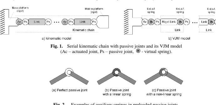
To describe most of existing parallel architectures, it is assumed that the general serial kinematic chain under study consists of a fixed “Base”, a number of flexible actuated joints “Ac”, a serial chain of flexible “Links”, a number of passive joints “Ps” and a moving “Platform” at the end (Fig. 1). It is also assumed that all links are separated by the joints (actuated or passive, rotational or translational) and their order is arbitrary. Besides, it is admitted that some links may be separated by actuated and passive joints simultaneously. Typical examples of the examined kinematic chains can be found in 3-PUU translational parallel kinematic machine [69], in Delta parallel robot [70] or in parallel manipulators of the Orthoglide family [52] and other manipulators[71]. It is worth mentioning that here a specific spatial arrangement of under-constrained chains yields the over-constrained mechanism that posses a high structural rigidity with respect to the external force.

Fig. 1. Serial kinematic chain with passive joints and its VJM model (Ac – actuated joint, Ps – passive joint, - virtual spring).

Fig. 2. Examples of auxiliary springs in preloaded passive joints.

To evaluate stiffness of the considered serial manipulator, let us apply a modification of the virtual joint method (VJM), which is based on the lump modeling approach [41]. According to this approach, the original rigid model should be extended by adding virtual joints (localized springs), which describe elastic deformations of the links. Besides, virtual springs are included in the actuating joints, to take into account stiffness of the control loop. Detailed description of such presentation as well as related assumptions are given in our previous publications [49, 67], where the kinematic model is presented as a product of homogeneous transformation matrices that after extraction of position and orientation of end-effector is transformed into the vector function [72]

( , )



t g q θ (1)

Here the vector t( ,p φ)T includes the position p ( ,x y z, )T and orientation φ ( _x,_y,_z)T of the end-platform (or end-effector) in the Cartesian space, the vector ( 1, 2, ..., )

T n

q q q



without internal preloading), the vector ( 1, 2, ..., )

T m

   

θ collects coordinates of all virtual joints and “preloaded passive

joints” (with auxiliary internal springs); n, m are the sizes of q and θ respectively.

Physical nature of passive joints with internal preloading is illustrated in Fig. 2. Such joints include internal springs, so their statics is described by the following expression



0



i K i i i

 

      (2)

where _i is the torque/force caused by deviation of the joint coordinate _i from its non-loaded (“zero”) value _{0 i}, and coefficient K_i defines the spring stiffness. For the purpose of generality, let us introduce similar “zero” values _{0 i} for the virtual springs that described flexibility of the links (obviously they are equal to zero for this subset of θ). This allows to define vector θ₀ of the same size as θ and to present the static equations corresponding to all variables (corresponding to perfect and preloaded passive joints, virtual springs of links and actuators) in general form τ K



θθ0



, τq 0. Here

, q 

τ τ are the generalized torque/force in joints corresponding to the variables θ and q, the matrix K_ collects stiffness coefficients of all springs of the kinematic chain.

It worth mentioning that in the case without internal preloading (see for example [49, 67]) the vector θ describes only flexibility of manipulator links/actuators that are presented by virtual springs, while vector qcollects entire set of passive joint coordinates. In contrast, in this paper, the passive joint coordinates are divided into two subsets: (i) “perfect passive joints” included in q, and (ii) “preloaded passive joints” included in θ together with traditional virtual springs. Besides, if a passive joint includes a nonlinear spring (see Fig. 2), the corresponding joint variable may be included either in θor q, depending on current configuration of manipulator. However, for each configuration, this assignment is strictly unique.

3.2 Problem statement

The designed stiffness model describes the resistance of manipulator to deformations caused by an external force or torque. It can be defined by the relation F f(Δt), where f(...) is a so-called “force-deflections” function that associates a deflection Δt with an external force F that causes the transition. It is worth mentioning that the function f(...) can de determined even for the singular configurations (or redundant kinematics) while the inverse statement is not generally true. Hence, enhanced stiffness analysis must include computing of this function and detailed analysis of its singularities that may provoke various nonlinear phenomena (such as buckling). In the unloaded case, this function is usually defined through the “stiffness matrix” K, which describes the linear relation

0 0

( , )

 

F K q θ Δt (3)

between small six-dimensional translational/rotational displacements Δt, and the external forces/torques F causing this transition. Here, it is assumed that Δt includes thee positional components



x, y,z



describing displacement in Cartesian space and three angular components



_x,_y, _z



that describe the end-platform rotation around the Cartesian axes, while the vectors q₀,θ₀ correspond to the manipulator equilibrium for which the loadings (both internal and external) are equal to zero. However, for the loaded mode, similar linear relation is defined in the neighborhood of

another static equilibrium, which corresponds to a different manipulator configuration ( , )q θ , that is modified by external forces/torques F. Respectively, in this case, the stiffness model describes the relation between the increments of the force

δFand the position δt

( , )

F

 

δF K q θ δt (4)

where qq₀Δq and θθ₀Δθ denote the new configuration of the manipulator, and Δ q, Δ θ are the deviations in the coordinates q θ, respectively.

Hence, the considered problem of enhanced stiffness analysis may be divided into several sequential subtasks:

(i) non-linear stiffness modeling that includes computing full-scale “force-deflections relation” for the externally loaded manipulator (taking into account internal preloading) and checking stability of corresponding equilibrium configurations;

(ii) linearization of the relevant force-deflection relations in the neighborhood of this equilibrium and computing corresponding stiffness matrix that in general case can be singular due to presence of passive joints;

(iii) determining the critical forces that may cause undesired buckling phenomena or sudden change of current configuration of the loaded manipulator.

4 Static equilibrium for the loaded mode

Computing of the static equilibrium is a key issue for the non-linear stiffness analysis, since it defines the manipulator configuration ( , )q θ required for the linearization of the “load-deflection” relation. In previous works, this issue was usually ignored and the linearization was performed in the neighborhood of the unloaded configuration assuming that the external load is small enough. It is obvious that the latter essentially limits relevant results and does not allow detecting non-linear effects such as buckling. From mathematical point of view, the problem is reduced to solving of a system of non-linear static equilibrium equations that may produce unique or non-unique, stable or unstable solutions.

4.1 Configuration of loaded manipulator

For computational reasons, let us consider the dual problem that deals with determining the external force F and the

manipulator equilibrium configuration ( ,q θ) that correspond to the end-effector location t taking into account internal preloading in the joints. Let us assume that the joints are given small, arbitrary virtual displacements q,θ in the neighborhood of ( ,q θ). According to the principle of virtual displacements, the virtual work of the external force F applied to the end-effector along the corresponding displacement  t J  θ Jq q is equal to the sum



T





T



q 

      

F J θ F J q (here J_ and J_qare the kinematic Jacobians with respect to the coordinates , q). Since the passive joints do not produce the force/torque reactions, the virtual work corresponding to the generalized forces/torques

, _q



τ τ includes only one component T



τ  θ (the minus sign takes into account the force-displacement directions for the virtual spring). In the static equilibrium, the total virtual work of all forces is equal to zero for any virtual displacement,

therefore the equilibrium conditions may be written as T

   

J F τ ; T

q  

J F 0, and taking into account assumptions and

notations from the previous section, the static equilibrium conditions can be presented as



0



; ; ( , )

T T

q

       

J F K θ θ J F 0 t g q θ (5)

where the vector θ₀ defines internal preloading in the joints, the matrix K_ describes stiffness of all springs in the adopted VJM model, while the external loading F and the configuration ( , )q θ are treated as an unknown for given end-effector location tg q θ( , ). Hence, the designed equilibrium configuration must satisfy the system of nonlinear equations (5).

It is evident that there is no general method for analytical solution of this system and it is required to apply numerical techniques. To derive the numerical algorithm, let us linearize the kinematic equation in the neighborhood of the current position (q θ_i, _i)

1 1

( _i, _i) _q( _i, _i) ( _{i i}) _( _i, _i) ( _{i i})

      

t g q θ J q θ q q J q θ θ θ (6)

and rewrite the static equilibrium equations as





1 1 0 1 ( , ) ; ( , ) T T i i i i q i i i           J q θ F K θ θ J q θ F 0, (7)

which leads to a system of linear algebraic equations with respect to (q_i1,θ_i1,F_i1) that includes the Jacobians J_(q θ_i, _i),

( , )

q i i

J q θ and geometrical location function g q θ( _i, _i) computed in the previous point (q θ_i, _i):

1 1 1 1 1 0 ( , ) ( , ) ( , ) ( , ) ( , ) ; ( , ) ( , ) q i i i i i i i i q i i i i i i T q i i i T i i i i                            J q θ q J q θ θ t g q θ J q θ q J q θ θ J q θ F 0 J q θ F K θ K θ (8)

This gives the following iterative scheme





1 1 1 1 0 ( , ) ( , ) , ( , ) ( , ) ( , ) 0 ( , ) i q i i i i i i q i i i i i i T i q i i T i i i                          _{  }                      F J q θ J q θ t g q θ J q θ q J q θ θ q J q θ θ J q θ K K θ (9)

that may be reduced down to 1 1 1 1 1 1 0 1 ( , ) ( , ) ( , ) ; ( , ) ( , ) 0 0 T i i i i i q i i i T i i i i T i q i i                                      F J q θ K J q θ J q θ ε θ K J q θ F θ q J q θ (10)

where ε_i  t g q θ( _i, _i)J q θ_q( _i, _i)q_iJ q θ_( _i, _i)θ_i. The latter is more convenient computationally, since it requires inversion of a lower dimension matrix



n6

 

 n6



instead of



nm6

 

 nm6



, where n, m are the sizes of the vectors q and θ respectively. For instance, for the kinematic chains of the Orthoglide manipulator (see example in section 6), expression (9) requires inversion of 3434 matrix, while iterative scheme (10) needs inversion of 1010

matrix only. It should be mentioned that 1



K is computed only ones, outside of the iterative loop.

Similar to other iterative schemes, convergence of this algorithm highly depends on the starting point. However, due to physical nature of the considered problem, it is possible to start iterations from the non-loaded configuration (q₀,θ₀). Besides, it is useful to modify the target point for each iteration in accordant with expression ti i t



1i



t0 using

scalar variable _i that is monotonically increasing from 0 up to 1. Another approach can be used for computing the

force-deflection curve. Here, the starting point can be taken from previously computed loaded configuration corresponding to another value of deflection that is very close to the target one. As it follows from computational experiments, for typical values of deformations the proposed iterative algorithm possesses rather good convergence (3-5 iterations are usually enough if a configuration is stable). In our simulation studies, the convergence was evaluated as the weighted sum of residual norms corresponding to equations (5) and the iterations were terminated when this criterion achieved prescribe value.

However, some computational difficulties may arise in the case of buckling or in the area of multiple equilibriums, where convergence problem becomes rather critical and highly depends on the initial guess. Here, number of iterations increase significantly and computational time becomes non-negligible. To overcome these difficulties, it is proposed to modify the developed iterative scheme and repeat computations several times, with slightly modified initial points that are obtained by adding small random noise to q₀,θ₀. Another option is adding small disturbances to



θ q_i, _i



at each iteration. These techniques were used in case studies presented section 6.

The proposed iterative scheme can be also slightly modified to solve the dual problem: computing an equilibrium configuration corresponding to given external loading F(instead of given t). In this case, expressions (9), (10) are used in internal loop, while the designed algorithm is supplemented by external loop, which provides iterative searching for t

corresponding to given F





1 1 i i i i       t t K F F (11)

where t_i,F_i and K_i are respectively the location, loading and stiffness matrix at the i-th iteration. It worth mentioning that the dual problem is meaningful only if the stiffness matrix K_i is non-singular. It is obvious that for a separate serial chain with passive joints the matrix K_i is always singular, while for the parallel manipulator it is usually non-singular due to specific assembling of kinematic chains. On the other hand, the original problem considered in this subsection (i.e.

computing F corresponding to t) is always physically meaningful and has at least one solution. More details concerning

the developed algorithms are contained in web-appendix to this paper, which includes pseudo-code versions of relevant procedures [74].

4.2 Stability of the loaded configuration

To investigate possible non-linear effects that may be caused by external and internal loading, it is necessary to extend the notion of stability associated with the stiffness analysis. Traditionally, the stability of compliant mechanical systems (including manipulators) is defined as resistance of end-point location t with respect to the “disturbing” effects of external force F applied at this point. In such formulation, the stability is completely defined by the stiffness matrix F

K that

describes linear relations (4) between the force and deflection deviations δ F δ t, with respect to the values F, t. It is

obvious that the matrix F

K is positive definite for the stable location t.

However, in compliant manipulators with passive joints, the configuration ( , )q θ corresponding to the same location t can be not unique. Moreover, these configurations may be both “stable” and “unstable” and correspond to different values of potential energy stored in the springs. From this point of view, it is worth to distinguish stability of end-point location t and stability of the corresponding configuration ( , )q θ . This issue becomes extremely important for the loaded mode, when due to kinematic redundancy caused by passive joints and excessive number of virtual springs, small disturbances in ( , )q θ

may provoke essential change of current equilibrium configuration that leads to reduction of the potential energy and transition to another equilibrium state, while keeping the same end-location. Hence, it is necessary to evaluate internal properties of the kinematic chain in the state of the loaded equilibrium that may correspond either to minimum or

maximum of potential energy for fixed value of t. Section 6 contains a number of illustrative examples that demonstrate

equilibrium bifurcations while incrementing the external loading, buckling phenomena and difference between two types of stability notions mentioned above. Also, additional animated illustrations describing this issue are available in web-appendix [74].

To evaluate stability of the static equilibrium configuration ( ,q θ), let us assume that the manipulator end-effector is fixed at the point t( ,p φ)T corresponding to the external load F, but the joint coordinates are given small virtual displacements q, θ satisfying the geometrical constraint (1), i.e.

( , ); ( , )

     

t g q θ t g q q θ θ (12)

For these assumptions, let us compute the total virtual work in the joints that must be positive for a stable equilibrium and negative for an unstable one. To achieve the virtual configuration (q q θ,  θ) and restore the equilibrium conditions, each of the joints must include virtual motors that generate the generalized forces/torques τq, τ which

satisfies the equations:



0



; ( ) ( 0 ) 0; ( ) T T T T q q q q                          J F K θ θ J J F K θ θ θ τ J F J J F τ (13)

After relevant transformations, the virtual torques may be expressed as

( T ) ; q ( Tq )

  

τ   J F K  θ τ   J F (14)

where (...) denotes the differential with respect to q, θ that may be expanded via Hessians of the scalar function

( , )T  g q θ F: ( T ) Fq F ; ( Tq ) Fq q qF  J F H   q H  θ  J F H   q H  θ (15) provided that 2 2 2 2 2 / ; / ; / F F F F q q          q  q      H q H θ H H q θ (16)

Further, taking into account that the virtual displacement from ( ,q θ) to (q q θ,  θ) leads to a gradual change of the virtual torques from (0, 0) to (τq,τ), the virtual work may be computed as a half of the corresponding scalar

products





1 2 T T q W _    τ    θ τ  q , (17)

where the minus sign takes into account the adopted conventions for the positive directions of the forces and displacements. Hence, after appropriate substitutions and transformation to the matrix form, the desired stability condition may be written as 1 0 2 F F q T T F F q q q W                 _   _       H K H θ θ q H H q (18)

where q and θ must satisfy to the geometrical constraints (12).

In order to take into account the relation between q and θ that is imposed by (12), let us apply the first-order expansion of the function g θ q( , ) that yields the following linear relation

q       _{ }   _   θ J J 0 q . (19)

Then, applying the SVD- factorization [73] of the integrated Jacobian

T r q q T q            _{ }            V S J J U U V 0 (20)

and extracting from V_, Vq the sub-matrices

o 

V , o

q

V corresponding to the zero singular values, a relevant null-space of

the system (19) may be presented as

o o

; q



 θ V  μ  q V  μ (21)

where μ is the arbitrary vector of the appropriate dimension (equal to the rank-deficiency of the integrated Jacobian). Hence, the stability condition (18) may be rewritten as an inequality

o o o o 1 0 2 T F F q T F F q q qq W                                     V H K H V μ μ V H H V (22)

that must be satisfied for all arbitrary non-zero μ. In other words, the considered static equilibrium ( ,q θ) is stable if (and only if) the matrix

o o o o 0 T F F q F F q q qq                                  V H K H V V H H V (23)

is negative-definite. It is worth mentioning that the obtained result is in a good agreement with previous studies [58], where

(for manipulators without passive joints) the stiffness properties were defined by the matrix F

 

K H that evidently must

be positive-definite for stable configurations. In Section 6 these results are applied for detecting bifurcations and buckling phenomena in typical serial kinematic chains and parallel manipulators.

5 Stiffness matrix for the loaded mode

The previous section presents technique that generally allows obtaining an exact relation between the elastic deformations and corresponding external force/torque. It is based on sequential computations of loaded equilibriums (and relevant force/torque) for various displacements of the manipulator end-point with respect to its unloaded location. However, though this relation is highly non-linear, common engineering practice operates with the stiffness matrix derived via the linearization.

To compute the desired stiffness matrix, let us consider the neighborhood of the loaded configuration and assume that the external force and the end-effector location are incremented by some small values F, t. Besides, let us assume that a new configuration also satisfies the equilibrium conditions. Hence, it is necessary to consider simultaneously two equilibriums corresponding to the manipulator state variables ( ,F q θ t, , ) and (F F q,  q θ,  θ t,  t). Relevant equations of statics may be written as



0



; 0 T T q        J F K θ θ J F (24) and



 















0 ; 0 T T                 θ θ θ q q J J F F K θ θ θ J J F F (25)

where J_q( ,q θ) and J_( ,q θ) are the differentials of the Jacobians due to changes in ( ,q θ). Besides, in the neighborhood of ( ,q θ), the kinematic equation may be also presented in the linearized form:

( , ) q( , )



   

δt J q θ δθ J q θ δq, (26)

Hence, after neglecting the high-order small terms and expanding the differentials via the Hessians of the function

( , )T

 g q θ F (similar to sub-section 4.2), equations (24), (25) may be rewritten as

( ) ( ) ( ) ( ) ( ) ( ) T F F q T F F q q q q                          J q , θ F H q , θ q H q , θ θ K θ J q , θ F H q , θ q H q , θ θ 0 (27)

and the general relation between the increments of the state variables can be presented as

q T F F q qq q T F F q               _{ } _           _ _  _{ }   0 J J F t J H H q 0 J H H K θ 0 (28)

The latter gives a straightforward numerical technique for computing the desired stiffness matrix: direct inversion of the matrix in the left-hand side of (28) and extracting from it the upper-left sub-matrix of size 66. Similarly, the matrices defining linear relations between the end-effector increment t and the increments of the joint variables θ, q can be computed, i.e.: ; ; C  q  F K  t  θ K  t  q K  t (29) where 1 * * C q T F F q q qq q T F F q                         _{ }  _      K 0 J J K J H H K J H H K (30)

It worth mentioning that the internal preloading (expressed by the variable θ₀) is not included in the latter expression in explicit way, but it directly influences on the variables ( ,q θ) describing the equilibrium configuration and corresponding Jacobians and Hessians, which are elements of (30). Besides, in contrast to previous works, here it is possible to obtain supplementary matrices K_,K_q that give additional measures of the manipulator stiffness which evaluate sensitivity of the joint coordinates ( ,q θ) with respect to the external loading.

In the case when the matrix inverse (30) is computationally hard, the variable θ can be eliminated analytically, using

corresponding static equation: F T F F

q

   

 θ k J   F k H  q, where F





1

   

F

k K H . This leads to a reduced system of

matrix equations with unknowns F and q

F T F F q T F F T F F F F q q q q q q                          _{     }              q θ J k J J J k H δF δt J H k J H H k H δq 0 . (31)

that may be treated in the similar way, i.e. the desired stiffness matrix is also obtained by direct inversion of the matrix in the left-hand side of (31) and extracting from it the upper-left sub-matrix of size 66:

1 F T F F C q q T F F T F F F F q q q qq q q                            _               K J k J J J k H K J H k J H H k H (32)

Similar to subsection 4.1, this approach allows reducing the dimension of the inverted matrix from



nm6

 

 nm6



to



n6

 

 n6



, that in the case of Orthoglide corresponds to 3434 and 1010respectively. It is worth mentioning that the structure of the latter matrix is similar to one obtained for the unloaded manipulator in [49] and differs only by Hessians that take into account the influence of the external load. It should also be noted that, because of the presence of the passive joints, the stiffness matrix of a separate serial kinematic chain is always singular, but aggregation of all the chains for a parallel manipulator produces a non-singular stiffness matrix. Some examples of such aggregation are presented in our previous papers [49, 67], where the stiffness matrices of separate kinematic chains are

expressed with respect to the same end-point and the resulting stiffness matrix for the parallel manipulator is computed as a

straightforward sum of these components, i.e. _C ( )_Ci

i





K K where the index „(i)‟ denotes the number of kinematic chain.

The later follows from the superposition principle, since the total external force corresponding to the same end-effector displacement is expressed as the sum of partial forces of the separate chains.

Further simplification can be obtained by applying the block matrix factorization technique (Frobenius equation) [75] that yields the following expression







 





 

 









 



1 1 1 1 1 F T F T F F C q q F F F F T F F T F T F F q q q q q q q q T F F T F T q q                                                                   K J k J J k J J J k H H H k H J H k J J k J J J k H J H k J J k J (33)

where the first term exactly corresponds to the classical formula defining stiffness of the kinematic chain without passive joints.

Hence, the presented technique allows computing the Cartesian stiffness matrix in the presence of the external and internal loading. It generalizes our previous results both for serial kinematic chains and for parallel manipulators [49,67]. In the following Section, it will be applied to several case-studies that deal with kinematic chains employed in typical parallel manipulators and demonstrate particularities of stiffness analysis of loaded manipulator with passive joints.

6 Illustrative examples

To demonstrate the efficiency of the proposed technique, let us present two examples that focus on the loaded working mode and deal with (i) the stiffness analysis of a serial kinematic chain with passive joints and (ii) the stiffness analysis of a translational parallel manipulator. Within this study, it is assumed that the external wrench is acting upon the manipulator end point and the influence of the gravity is negligible. In previous works [49,67], this problem was studied for the unloaded working mode and/or for small deflections in elastic elements, so any non-linear abnormality in the manipulator behavior (buckling, etc.) was non detected. This Section includes only summary of this computational study, while more details are presented in web-appendix [74]

6.1 Stiffness analysis of a serial kinematic chain

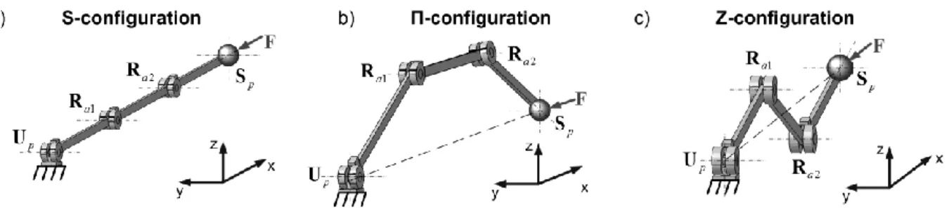
First, let us consider a serial kinematic chain consisting of three similar links separated by two similar rotating actuated joints. It is assumed that the chain is a part of a parallel manipulator and it is connected to the robot base via a universal passive joint, and the end-platform connection is achieved via a spherical passive joint. For each of these configurations, let us investigate three types of the virtual springs corresponding to different physical assumptions concerning the stiffness properties of the actuators/links. They cover the cases, in which the main flexibility is caused by the torsion in the actuators, by the link bending, and by the combination of elementary deformations of the links.

6.1.1 Geometric model

The geometry of the examined kinematic chain (Fig. 3) can be defined as UpRaRaSp where R, U and S denote

respectively the rotational, universal and spherical joints, and the subscripts „p‟ and „a’ refer to the passive and active joints respectively. Using the homogeneous matrix transformations, it can be described by the equation

0 1 1 2 2 3

( ) ( ) ( ) ( ) ( ) ( ) ( ) ( ) ( ) ( )

u x L s z qa x L s z qa x L s s t

         

T R q T T θ R T T θ R T T θ R q (34)

where R_z(...) and T_x(...) are the elementary rotation/translation matrices around/along the z- and x-axes, R_u(...) is the homogeneous rotation matrix of the universal joint (incorporating two elementary rotations), R_s(...)is the homogeneous rotation matrix of the spherical joint (incorporating three elementary rotations), q_a1, q_a2 are the coordinates of the actuated joints, L is the length of the links, q₀is the coordinate vector of the universal passive joint located at the robot base, q_t is the coordinate vector corresponding to the passive spherical joint at the end-platform, T_s(.) is the homogenous matrix-function describing elastic deformations in the links and actuators (they are represented by the virtual coordinates incorporated in the vectors θ θ₁, ₂,θ₃). It is obvious that this model can be easily transformed into the form tg q θ( , )

Fig. 3. Examined kinematical chain and its typical configurations

( Up – passive universal joint, Ra1, Ra2 – actuated rotating joints, Sp – passive spherical joint)

To investigate particularities of this kinematic chain with respect to the external loading, let us also consider three typical postures that differ in values of the actuated coordinates:

 S-configuration: the links are located along the straight line (Fig. 3a),

the actuated coordinates are qa1 qq2 0

 -configuration: the chain takes a trapezoid shape (Fig. 3b),

the actuated coordinates are qa1 qq2  3 0 

 Z-configuration: the chain takes a zig-zag shape (Fig. 3c),

the actuated coordinates are qa1  qq2 3 0 

For presentation convenience, let us also assume that the coordinates q₀ of the universal passive joint are computed to ensure location of the end-effector on the Cartesian axis x. Besides, it is assumed that the external loading is presented by a compressing force applied at the chain end-point and it is directed along x-axis (see Fig. 3).

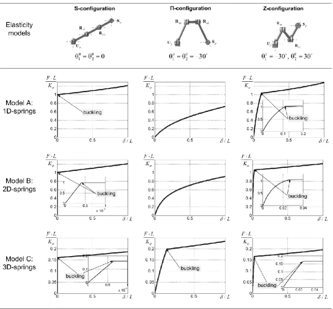
6.1.2 Stiffness models

In order to investigate possible non-linear effects in the stiffness behavior of this chain, let us consider several cases that differ in stiffness models of the links and actuated joints:

Case of 1D-springs (Model A): the flexible elements are localized in the actuating drives while the links are

considered as strictly rigid. It allows, without loss of generality, to reduce the original UpRaRaSp model down to RpRaRaRp

and define a single stiffness parameter K_ (similar for both actuators) that will be used as a reference value for the further analysis. Besides, it is possible to ignore the end-effector orientation and consider a single passive joint coordinate q (at the base) and two virtual joint coordinates ₁, ₂ (at actuators).

Case of 2D springs (Model B): the actuators do not include flexible components but the manipulator links are subject

to non-negligible elastic deformations in Cartesian xy-plane (bending and compression). Correspondingly, the link flexibility is defined by a 33 matrix that includes elements describing deformation in x- and y- directions and rotational deformation with respect to z-axis.

Case of 3D springs (Model C): the actuators are strictly rigid but the link flexibility is described by a full-scale 3D

model that incorporates all deflections along and around x-,y-,z-axes of the three-dimensional Cartesian space. Relevant stiffness matrix of the links has the dimension 66. The kinematics of this model corresponds to the general expression UpRaRaSp, it includes two passive joints



q q, s



incorporating in total five passive coordinates and three virtual-springs

with 18 virtual coordinates totally (six for each link).

6.1.3 Stiffness analysis for model A

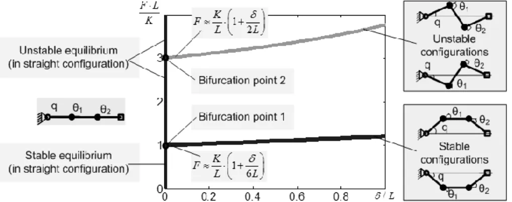
In this case, the model includes minimum number of flexible elements (two 1D virtual springs in the actuated joints) and may be tackled analytically. However, in spite of its simplicity, it is potentially capable to detect the buckling phenomena at least for S-configuration, because of evident mechanical analogy to straight columns behavior under axial compression. It is also useful to evaluate other initial configurations (- and Z-types), their stability and to compare

analytical solutions with numerical results provided by the developed technique.

For this model, consistent solution of geometrical and static equations (5) yields two expressions for “force-deflection” relations that correspond to stable and unstable equilibriums

 

sin s K F L      ;

 

cos( ) 2 cos sin n K q q F L            (35)

where F are the force acting along the x-axis,  is corresponding linear displacement, the subscripts „s‟ and „n‟ denote manipulator configuration stability (stable or unstable), K_ is actuator stiffness, L is the length of the links, and auxiliary