The convergence of a neuromuscular impulse response towards a lognormal, from theory to practice

Auteurs:

Authors: Réjean Plamondon, Chunhua Feng et Moussa Djioua

Date: 2008

Type: Rapport / Report

Référence:

Citation:

Plamondon, Réjean, Feng, Chunhua et Djioua, Moussa (2008). The Convergence of a Neuromuscular Impulse Response Towards a Lognormal, from Theory to Practice. Rapport technique. EPM-RT-2008-08.

Document en libre accès dans PolyPublie

Open Access document in PolyPublie

URL de PolyPublie:

PolyPublie URL: http://publications.polymtl.ca/2630/

Version: Version officielle de l'éditeur / Published version_{Non révisé par les pairs / Unrefereed} Conditions d’utilisation:

Terms of Use: Autre / Other

Document publié chez l’éditeur officiel

Document issued by the official publisher

Maison d’édition:

Publisher: École Polytechnique de Montréal

URL officiel:

Official URL: http://publications.polymtl.ca/2630/

Mention légale:

Legal notice: Tous droits réservés / All rights reserved

Ce fichier a été téléchargé à partir de PolyPublie, le dépôt institutionnel de Polytechnique Montréal

This file has been downloaded from PolyPublie, the institutional repository of Polytechnique Montréal

THE CONVERGENCE OF A NEUROMUSCULAR IPULSE RESPONSE TOWARDS A LOGNORMAL, FROM

THEORY TO PRACTICE

Réjean Plamondon, Chunhua Feng et Moussa Djioua Département de Génie électrique,

Laboratoire Scribens, École Polytechnique de Montréal

EPM-RT-2008-08

The Convergence of a Neuromuscular Impulse

Response Towards a Lognormal, from Theory to

Practice

Réjean PLAMONDON, Chunhua FENG et Moussa DJIOUA

Département de Génie Électrique,

Laboratoire Scribens,

École Polytechnique de Montréal.

©2008

Réjean Plamondon, Chunhua Feng, Moussa Djioua,

Tous droits réservés

Dépôt légal :

Bibliothèque nationale du Québec, 2008 Bibliothèque nationale du Canada, 2008 EPM-RT-2008-08

The Convergence of a Neuromuscular Impulse Response Towards a Lognormal, from Theory to Practice

: Réjean Plamondon, Chunhua Feng, Moussa Djioua Département de génie électrique, Laboratoire Scribens

École Polytechnique de Montréal

Toute reproduction de ce document à des fins d'étude personnelle ou de recherche est autorisée à la condition que la citation ci-dessus y soit mentionnée.

Tout autre usage doit faire l'objet d'une autorisation écrite des auteurs. Les demandes peuvent être adressées directement aux auteurs (consulter le bottin sur le site http://www.polymtl.ca/) ou par l'entremise de la Bibliothèque :

École Polytechnique de Montréal

Bibliothèque – Service de fourniture de documents Case postale 6079, Succursale «Centre-Ville» Montréal (Québec)

Canada H3C 3A7

Téléphone : (514) 340-4846

Télécopie : (514) 340-4026

Courrier électronique : biblio.sfd@courriel.polymtl.ca

Ce rapport technique peut-être repéré par auteur et par titre dans le catalogue de la Bibliothèque : http://www.polymtl.ca/biblio/catalogue/

Abstract: Lognormal functions have been found among the best descriptors of the impulse re-sponse of neuromuscular systems under various experimental conditions. This arises from the fact that lognormal patterns automatically emerge when a large number of coupled systems inter-act to produce a response. This paper evaluates the error of convergence towards a lognormal. Under the umbrella of the Central Limit Theorem, the error functions for lognormal and delta-lognormal equations are derived and analyzed. It is shown that these errors can be computed from the estimated values of the lognormal parameters, without any explicit reference to the number of subsystems involved. The resulting theoretical framework is then exploited in three applications: the comparative benchmarking of parameter extraction algorithms, the validation of the results in analysis-by-synthesis experiments and the estimation of the range of acceptable movement times in tests involving rapid movements.

1. Introduction

Computational models have been used for many years to study, characterize and com-prehend human motor control. From a movement execution perspective, most of these models can be depicted as systems that perform a mapping from a task space to an action space. In this context, these various models can be classified according to their task representation (action plans, virtual targets, terminal attractors, optimization criteria, equilibrium points, etc.), their mapping processes (a wide range of methods, from a network of differential equations to compact analytical expressions) or their action spaces (dynamics, kinematics, statics, etc.). Each model encompasses the benefits as well as the limitations of its own interpretation scheme and it is im-portant to study a model in details to better delimit its zone of validity and its domains of applica-tion. In this paper, we pursue our analysis of such a model to further circumscribe its practical use

and propose new potential implementations. Indeed, we have demonstrated in this Journal (Pla-mondon et al. (2003) that the impulse response of a neuromuscular system converges toward a lognormal function under some very general conditions. Assuming that the cumulative time de-lays of a sequence of dependent sub-processes constituting a neuromuscular system were gov-erned by a law of proportionate effects, it has been proved, using the Central Limit Theorem, that a neuromuscular system can be described globally as a linear system having a lognormal impulse response.

The use of a lognormal function to describe the impulse response of a neuromuscular sys-tem constitutes the corner stone of the Kinematic Theory of rapid human movements (Plamondon 1995a, b, 1998). According to this framework, a rapid movement towards a target is produced by a synergy made up of two neuromuscular systems, an agonist system acting in the direction of the target and an antagonist one working in the opposite direction. When the two systems act in per-fect opposition, the magnitude of the velocity profile can be described by a delta-lognormal equa-tion:

(

)

2 0 = ( 0) = 1 1( ; , , )0 1 1 2 2( ; , ,0 2 v t t t t D t t D t t 2 2) μ σ − ΔΛ − Λ − Λ r _{μ σ (1)} where 2 (ln( 0 2 2 0 ) ) 1 2 ( ; , , ) = , = 1,2 2 t t _i i i i i i t t e i μ σ μ σ σ π − − − Λ (2)

with 2 : the impulse response of a neuromuscular system. 0 ( ; , , )( = 1,2) i t t μ σi i i Λ ( = 1,2) i

D i : the magnitude of the input commands to the system. _ith

0

( = 1,2)

i i

μ : the logtime delay of the system. _ith

( = 1,2)

i i

σ : the logresponse time of the system. _ith

When the two systems do not act in perfect opposition, the vectorial version of the model must be used (Plamondon and Djioua 2005, 2006) and the velocity profile is described by a weighted sum of lognormals:

2 0 0 =1 =1 ( ) = n _i( _i) = n _i ( ; , , ),_{i i} 2 i i v t

∑

v t t−

∑

D t tΛ μ σ n r ur uur ≥ (3)

where is the vectorial input command to the system. urDi ith

Using similar approaches, lognormal functions have also been used to describe complex 2D movements like handwriting (Plamondon and Guerfali 1998) as well as 3D movements (Leduc and Plamondon 2001).

To summarize, in the context of the previous classification scheme, the Kinematic Theory describes a movement using action plans made up of a sequence of virtual targets (urD1i, Dur2i, ). These plans are instantiated through the lognormal impulse response of the selected neuromuscu-lar systems (characterized by

0i

t

1i

μ ,μ2i,σ1i,σ2i) and the overall result is described in the kinematic domain using the velocity profile of the end-effector.

Over the years, the Kinematic Theory has been employed to describe and explain under a single umbrella a large body of experimental data consistently reported in the field (Plamondon 1995a,b, 1998; Plamondon and Alimi 1997; Alimi and Plamondon 1996, 1994; Woch and Pla-mondon 2004; PlaPla-mondon and Djioua 2005; Woch and PlaPla-mondon 2007). Among other things, for unidimensional movements, the theory accounts for:

• The asymmetric bell-shaped of the velocity profile (Georgopoulos et al 1981, Morasso 1981, Soechting and Laquantini 1981, Abend et al 1982, Atkeson and Hollerbach 1985, Nagasaki 1989, Uno et al 1989, Berardelli et al. 1996).

• The decrease of asymmetry as a function of velocity (Beggs and Howarth 1972), of spatial and temporal constraints (Shapiro and Walter 1986, Cooke and Brown 1994, Schmidt and Lee 1999) and its inversion at very high speed (Zelaznik et al 1986).

• The rescalability or non-rescalability of the velocity profiles under diverse experimental condi-tions (Gielen et al 1985, Mustard and Lee 1987, Corcos et al 1990, Brown and Cooke 1981,1990, Gottlieb et al 1989, Goggin 1990).

• The relationship between numerous global variables (maximum velocity, time to maximum velocity vs. movement time or movement amplitude) under a variety of experimental protocols (Jeannerod 1984, Lestienne 1979, Hoffman and Strick 1986, Milner 1986, Wadman et al 1979, Brown and Slatter-Hammel 1949, Brook 1974, Freund and Budingen 1978).

• The different types of speed-accuracy tradeoffs (Fitts 1954, Schmidt et al 1979, Newell et al 1979, Howarth et al 1971, Wright and Meyer 1983, Hancock and Newell 1985).

• The various properties of isotonic and isometric forces patterns (Gielen et al 1985, Gottlieb et al 1990, Marteniuk et al 1990, Freund and Büdingen 1978, Ghez and Gordon 1987).

• The variability of many global variables (peak velocity, peak acceleration, maximum isometric and isotonic forces) (Gielen et al 1985, Nagasaki 1989, Carlton and Newell 1988, Sherwood and Schmidt 1980, Gordon and Ghez 1987).

A recent theoretical study has even shown that among the class of models that exploit analytical expressions to describe velocity profiles, the Delta-Lognormal model can be consid-ered as the ultimate model toward which the Minimum-Jerk, the Minimum-Time, the Beta and

the Gamma models converge (Djioua and Plamondon 2007). In this perspective, the Kinematic Theory can be seen as an ultimate analytical minimization theory, aiming at minimizing the en-ergy associated to the convergence error. From a practical point of view, the exploitation of the Kinematic Theory relies on the ability to extract the delta-lognormal parameters from real move-ments using analysis-by-synthesis experimove-ments. So far, the delta-lognormal functions have lead to the best reproduction of unidimensional movements, with a minimum of errors (Plamondon et al 1993, Alimi and Plamondon 1994, Alimi 1994, Feng et al. 2002), which suggests that the con-vergence error is probably very small. But, the search for optimal solutions remains an open problem and sub-optimal solutions can be found acceptable in many applications (Djioua et al., 2005,2007b), provided that these solutions can be quantitatively evaluated with proper limiting criteria and thresholds .

In this paper, we track this evaluation problem, using the error of convergence toward a lognormal as a guideline, to assess, among other things, the quality of parameter estimations. One important result of this theoretical study is that the error can be directly computed from the esti-mated values of the lognormal parameters without any explicit reference to the number of subsys-tems involved. Although, the total reconstruction errors come from both experimental and theo-retical sources, it is shown that the theotheo-retical predictions constitute a lower bound that can be used in practical applications.

In the next section, we derive the analytical expression for the lognormal convergence er-ror. In section 3, we present some computer simulations to analyze this error function. In section 4, our results are generalized to the case of delta-lognormal velocity profiles and we also analyze a few simulations. In the next two sections, we report on some experimental results obtained from

the analysis-by-synthesis of simulated data (section 5) and real human movements (section 6), and we discuss the interest of using the convergence error in three practical applications:

• The comparative benchmarking of delta-lognormal parameter extraction algorithms, • The definition of a threshold for the validation of parameter extraction results, • The definition of an acceptable range of movement times in a typical experiment on rapid movements.

2. Convergence error for the lognormal

The proof of lognormal convergence (Plamondon et al 2003; Feng 2005) is based on the representation of the impulse response of a neuromuscular system h t t )( − 0 as the limit to the convolution of impulse responses N h t t )i( − 0 of time coupled sub-processes describing that sys-tem, on a logarithmic time scale. As tends toward infinity, N

(4) 0 1 0 2 0 0 ( ) = _lim ( ) ( ) _N( ) = _{lim N}( N N h t t h t t h t t h t t h t t →∞ →∞ − − ∗ − ∗ ∗_L − % − ₀₎

tends toward a lognormal function 2 0

( ; , , )t t μ σ

Λ .

What is of interest here is the error of convergence of h t t%_N( − ₀)_:

2

0 0 0

( ) = ( ) ( ; , ,

N N

Err t t− h t t% − − Λ t t μ σ ) ₍₅₎

We present in the following paragraphs the major steps to get an analytical expression for . The complete details of the proof are given in the Appendix.

0 (

N

To derive the mathematical equation for Err t t )_N( − ₀ , we must first make a change of variable l = ln(t t− ₀) that convert the lognormal convergence of h t t )%_N( − ₀

( )

l

H

into the normal con-vergence of ( )l . We then move to the frequency domain, using

N

h e% % ω _{the Fourier transform}

of h e%_N( l₎: 1 2 1 2 1 2 ( ) = ( ) ( ) ( ) ( ) ( ) ( ) = ( ) ( ) ( ) l l l lN j_l j_l j l l lN H H H H A eφ A eφ A eφ ω ω ω ω lN ω ω ω ω ω % _L L ω (6) where for i= 1, ,L N, 2 2 2 4 2 4 2 ( ) = 1 2! 4! i i i li A σ e ω σ σ ω − ω + ω _{+L ;} − (7) 3 3 5 5 1 ( ) = 3!i 5!i li i μ μ φ ω −μ ω+ ω − ω _+L (8)

For simplicity, we make a change of variable such that the first moment μ1i = 0, thus

3 5 3 5 ( ) = ,mod.2 = 1, , . 3!i 5!i li ini N μ μ φ ω ω − ω _{+L L} (9) Then we have 1 2 1 2 ( 1 2 1 2 2 2 _{3 3 5 5} ( ( ) ( ) ( ) ( ) = ( ) ( ) ( ) ( ) ( ) ( )) = ( ) ( ) ( ) ) 3! 5! 2 = j_l j_l j_lN l l l lN j l l lN l l lN j H A e A e A e A A A e e e φ φ φ φ μ σ ω ω ω ω ω ω ω ω φ ω φ ω ω ω ω μ ω _{ω ω} − + + + − + % _L L L L (10)

where 2 2 3 3 =1 =1 = _iN _i, = N_{i i} σ

∑

σ μ

∑

μ and μ₅ =

∑

_iN₌₁μ_5i. Noting that 5 3 5 3 ( 3 5 3 5 2 3 5 3 5 ) ₁ 3! 5! _{= 1 ( ) ( )} 6 5! 2! 6 5! j j j j j e μ _ω μ _ω μ ω μ ω μ ω μ ω − + + − + + − + + L L L L (11) We obtain 2 2 3 5 3 5 2 3 5 3 5 2 2 2 2 2 2 2 2 2 2 3 5 3 5 2 2 3 5 3 5 1 2 ( ) = [1 ( ) ( ) ] 6 5! 2! 6 5! 1 1 2 2 2 2 2 = ( ) 6 5! 2! 6 2! 5! l j j j j H e j j j j e e e e e σ σ σ σ σ σ ( ) ω μ ω μ ω μ ω μ ω ω ω ω ω ω ω μ ω μ ω μ ω μ ω − − − − − − + − + + − + + + − + + % _{L L L} L + (12) So we can use 2 2 3 3 2 6 jμ ω _e−σ ω

as an approximation of the error in Fourier domain under

the previous change of variables. Since the inverse transform of the function

2 2 3 3 2 6 jμ ω _e−σ ω is: 2 2 2 3 3 ₂ 3 3 3 1 ₂ 1 ₂ ( ) = = 2 6 6 2 x j x j x x f x e e d e σ ω 3 ω μ ω _ω μ _σ π σ π − − ∞ −∞ σ σ ⎡ _{⎛ ⎞} ⎤ ⋅ ⋅ _⎢− +_{⎜ ⎟ ⎥} ⎝ ⎠ ⎢ ⎥ ⎣ ⎦

∫

(13)

we can now return to the case where the first moment = ₌₁ 1

N i i

μ

∑

μ is not zero. Noting that the Fourier transform of the function

2 2 1 _exp( ( ₎ 2 2 l μ σ σ π − − ) (14) is 2 2 exp( )exp( ) 2 j σ ω _μω − − (15)

and that the transform of

2 3 2 1 _exp( ( ) _)[ 3( ) ( _] 2 2 l l l 3 ) μ μ μ σ σ σ σ π − − − − − + (16) is 2 2 3 exp( )exp( ) ( ) 2 j j σ ω _{μω σω} − − (17)

therefore, making the inverse transform of the function H%_l( )ω , we get the error ap-proximation formula: 2 2 2 3 3 2 3 1 ( ) ( ) = ( ) exp( ) 2 2 1 _exp( ( ) _)[ 3( ) ( ) _] 6 2 2 l l N N l Err e h e l l l μ σ σ π μ _{μ μ μ} 3 σ σ π σ σ − − − − − − ⋅ − − + % ; σ (18)

2 3 3 0 0 0 3 2 0 (ln( ) ) 3(ln( ) ) (ln( ) ) 1 ( ) exp( )[ 6 2 ( ) 2 N t t t t t t Err t t t t 0 3 ] μ μ μ σ σ π σ σ − − − − − − − ⋅ − − + − ; μ σ ) (19)

If the lognormal impulse response is activated with an input command , then the out-put of the system is the component of a velocity profile:

D 0 ( N v t t_% −

(

)

(

2

)

(

)

0 = ; , ,0 N _N v t t_% − D t tΛ μ σ +Err t t_v − ₀ ) (20)

and the error Err t t_vN( − ₀ on this profile can be described by:

2 0 0 0 2 0 2 3 30 0 0 2 3 3 0 0 (ln( ) ) ( ) = ( ) exp( ) 2 2 ( ) (ln( ) ) 3(ln( ) ) (ln( ) ) = exp( )[ 2 6 2 ( ) v_N N D t t Err t t v t t t t t t t t t t D N t t μ σ σ π μ 0 _] μ μ μ σ σ σ σ σ π − − − − − − − − − − − − − ⋅ − − + − % (21)

3. Computer simulations

Apart from , that reflects a time translation and , an amplitude scaling factor, the ef-fect of the two other lognormal parameters on the convergence error (19) is better understood with simulations. Figure 1a highlights the effect of

0

t D

μ, the logtime delay, on (equation 20) and Figure 1b depicts the global effect of

0 (

N

v t t_% − )

μ on Err_vN(t−t₀)(equation 21) by illustrating how its global mean square value (MSE) changes with μ . As μ gets smaller (faster movements), the

velocity component increases in peak amplitude and its width is reduced (see Figure 1a). This reduction of μ has a tendency to decrease the MSE that is, the energy associated with the error function (see Figure 1b). In other words, for a neuromuscular system, the shorter are the time de-lays, the faster is the convergence and the smaller is the convergence error.

-1.60 -1.4 -1.2 -1 -0.8 -0.6 -0.4 -0.2 0.05 0.1 0.15 0.2 0.25 0.3 0.35 μ En er gy of th e Er ro r f unct ion 0 140 120 0.2 0.4 0.6 0.8 1 1.2 0 20 40 60 80 100 Decrease of μ values time [s] vN (t-t0 ) [m .s -1]

Figure.1 Effects of μ on the velocity component v t t )_%N( − ₀ and on the energy associ-ated with the error function ( ₀ . As

N t t− ) v

Err μ decreases, the effects of the error diminish.

0 0.2 0.4 0.6 0.8 1 0 20 40 60 80 100 120 140 160 180 Time [s] vN (t-t0 ) [ cm. s -1] Decrease of σ values 0.05 0.1 0.15 0.2 0.25 0.3 0.01 0.02 0.03 0.04 0.05 0.06 0.07 0.08 0.09 σ Ener gy of the E rr or fun ct ion

Figure.2 Effects of σ on the velocity component v t t )_%N( − ₀ , and on the energy associated with the error function Err_v ( −t₀). As

Figures 2 highlight the effect of σ under similar conditions. As expected, a smaller value of σ results in an increase of the peak amplitude of v t t )_%N( − ₀ and a reduction of its width (see Figure 2a). This reduction in logresponse time has a tendency to decrease the energy associated with the error function that is, the faster is the response time, the smaller is the MSE (see Figure 2b). One must notice that these effects are very small, when compared to the ampli-tudes of the velocity components, but they might be at the basis of several phenomena that are observed in rapid movements. For example, longer time delays (increase of

0 (

vN

Err t t− )

μ and σ), a charac-teristic of movements made by aged subjects (Woch and Plamondon 2007a), will result in larger convergence errors and thus more tremors in the signal.

4. The delta-lognormal convergence

In many applications, particularly when working with fast single unidirectional move-ments, it has been shown that equation (3) reduces to the delta-lognormal equation (1) (Plamon-don and Djioua 2006). Since a delta-lognormal is the difference of two lognormal impulse re-sponses weighted by their respective input commands, the total convergence error of this velocity can then be obtained by subtraction. Indeed, if 0

1( )

vN

Err t t− represents the agonist lognormal er-ror and ₀ represents the antagonist lognormal error, that is:

2( vN Err t t− ) 2 (ln( 0 1 2 1 1 0 ₁ 0 1 _{1 0} ) ) 2 ( ) = ( ) 2 ( ) t t v_N N D Err t t v t t e t t μ σ σ π − − − − − − − % (22) and,

2 (ln( 0 2 2 2 2 0 ₂ 0 2 _{2 0} ) ) 2 ( ) = ( ) 2 ( ) t t v_N N D Err t t v t t e t t μ σ σ π − − − − − − − % (23)

then, with being the velocity profile of rapid movement and 0 ₁ 0 ₂ ( ) = _N ( ) _N ( v t t_% − v t t_% − −v t t_% 2 1 ( ; , , )t t0 1 1 D2 ( ; , , )t t0 2 2 0) − 2 ( ;...) =t DΛ μ σ − Λ μ σ

ΔΛ , its corresponding ideal delta-lognormal de-scription, the delta-lognormal convergence error can be described by:

0 ₁ 0 ₂ 0 2 2 (ln( _{0 1} (ln( _{0 2} 2 2 1 1 2 2 1 0 2 0 ( ) = ( ) ( ) ) ) ) ) 2 2 _, 2 ( ) 2 ( ) v N N t t t t Err t t v t t v t t D _e D _e t t t t μ μ σ σ σ π σ π − − − − ⎡ ⎤ − _⎣ − − − _⎦− − − ⎡ ⎤ ⎢ ⎥ − ⎢ ⎥ − − ⎢ ⎥ ⎢ ⎥ ⎣ ⎦ % % (24) namely 2 (ln( 0 1 3 2 31 1 1 0 1 0 1 0 3 3 1 1 0 1 2 (ln( 0 2 3 2 32 2 2 0 2 0 2 3 3 2 2 0 2 ) ) 3(ln( ) ) (ln( ) ) 2 ( ) [ ] 6 2 ( ) ) ) 3(ln( ) ) (ln( ) ) 2 _{[ ]} 6 2 ( ) t t v t t t t t t D Err t t e t t t t t t D _e t t 1 2 μ μ σ μ σ σ π σ μ μ σ μ σ σ π σ − − − − μ σ μ σ − − − − − − ⋅ − + − − − − − − − ⋅ − + − ; (25)

We have performed computer simulations to study this latter equation. We have plotted in Figure 3a, a delta-lognormal velocity pattern, with typical values of ,μ σ_{i i}, and its two lognormal components. In Figure 3b, the total delta-lognormal error with its agonist and antagonist compo-nents are depicted. As can be seen, the agonist error is more important than the antagonist one and this latter has the tendency to increase the total error because of the different timing between these two signal components. Here again, from an energy perspective, the global effect of the convergence error increases as the movements get slower (larger μ and σ ).

0 0.1 0.2 0.3 0.4 0.5 0.6 0.7 -50 0 50 100 Time [s] v(t-t 0 ) [ cm .s -1] Delta-lognormal Agonist lognormal Antagonist lognormal 0 0.1 0.2 0.3 0.4 0.5 0.6 0.7 -0.4 -0.3 -0.2 -0.1 0 0.1 0.2 0.3 Time [s] Er rv (t-t0 ) [c m .s -1] Delta-lognormal error Agonist error Antagonist error

Figure.3 Typical example of a delta-lognormal profile 2

0 0

( ) = ( ; , ,

v t t− D t tΛ μ σ ) and its total error of convergenceErr t t_v( − ₀). The individual components are also plotted in each graph.

5. Working with simulated data

5.1 Practical application I: Benchmarking of parameter extraction algorithms

A first application of the present study is to evaluate the sensitivity of a specific parame-ter extraction algorithm to the convergence error. To do so, a database of ideal delta-lognormal profiles (equation 1) and a database of noisy profiles that incorporate their respective conver-gence error (equation 25) have been built (Plamondon, Li and Djioua 2007; Djioua and Plamon-don 2008). To have a database that reflects the large variety of velocity profiles encountered in real experiments, we have created seven classes of signals, each class containing 1000 speci-mens. A class is identified by the number of peaks in the velocity profile ( or i if no real roots) and the position of the antagonist component dominance with respect to the agonist one ( (before) , (after) or (simultaneous)).Each curve, ideal and noisy has been

proc-uv

C v= 0,1,2

=

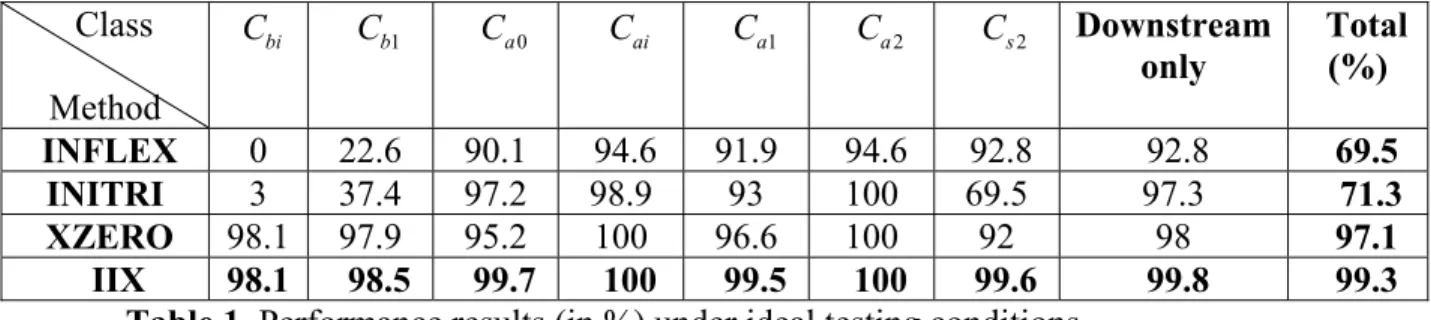
essed by three parameter extraction algorithms currently available in our laboratory: INFLEX (Guerfali and Plamondon 1995), INITRI (Plamondon, Li and Djioua, 2007) and XZERO (Djioua and Plamondon, 2008). We have also tested a system that combines the three previous algorithms in parallel and keeps the best solution (the IIX system). We have summarized in Tables 1 and 2 the results of these tests for the ideal and noisy conditions. For each algorithm and for each class of curves, the percentages of convergence toward the exact solution (known from our truth table) within a SNR greater than 50dB are reported.

1 C

Table 1. Performance results (in %) under ideal testing conditions Class Method bi C Cb1 Ca0 Cai Ca1 Ca2 C Downstream s2 only Total (%) INFLEX 0 22.6 90.1 94.6 91.9 94.6 92.8 92.8 69.5 INITRI 3 37.4 97.2 98.9 93 100 69.5 97.3 71.3 XZERO 98.1 97.9 95.2 100 96.6 100 92 98 97.1 IIX 98.1 98.5 99.7 100 99.5 100 99.6 99.8 99.3 (Performance criterion : SNR≥50dB ) Class Method C_bi C_b a0 Cai Ca1 Ca2 C Downstream s2 only Total (%) INFLEX 0 24.6 89 94.1 91.2 94.6 92.1 92.2 69.4 INITRI 0.3 37.4 97.5 97.6 93.4 100 69.6 97.1 70.8 XZERO 99.9 87.0 91.9 100 84.4.6 100 97.4 94.1 94.4 IIX 99.9 93.8 99.6 100 99.2 100 99.7 99.7 98.9

Table 2. Performance results (in %) under noisy testing conditions (Performance criterion : SNR≥50dB )

As one can see from Table 1, none of the algorithms is perfect: INFLEX and INITRI have problems with the C_bi and theC_b1 classes (upstream cases), while INITRI performs better than

XZERO on the class. Although, XZERO is the best algorithm, the combination of the three methods into the IIX system leads to the best performances. Comparing the columns of the two Tables, one can see that all the algorithms are slightly affected by the convergence error some-times positively somesome-times negatively, depending on the class of curves. On a global basis, com-paring the last columns of the two Tables, we can see that XZERO is more sensitive to the error of convergence although it performances still greatly exceed the two others. Here again, the com-bined IIX system is the most robust and should be preferred. In a more general perspective, these results set the pass mark for the search of a new algorithm.

1

a

C

6. Working with real data

6.1. Typical experimental results

To get a more realistic picture, we have run an analysis-by-synthesis experiment on real data previously collected according to the following scenario: ten (10) healthy young subjects, sitting in a comfortable position, were required to produce rapid strokes on a digitizer with their dominant hand. The ( ), ( )x t y t trajectory, sampled at Hz, was then processed to compute the velocity profile of the pen tip.

200

For each profile, the nonlinear regression system IIX (Djioua 2007, Djioua and Plamon-don 2008) was used to extract the best set of seven parameters that allow a reconstruction of the velocity with a minimum of errors. We have plotted in Figure 4 a typical result of such an ex-periment. Figure 4a shows a typical stroke trajectory, as collected on the digitizer. In Figure 4b, one can see the original velocity profile, its ideal delta-lognormal reconstruction and its two com-ponents. The reconstruction error was quantified with the Mean Square Error (MSE) and the

Sig-nal to Noise Ratio (SNR). Figure 4c depicts the time course of the total reconstruction errors ( ) as well as the theoretical convergence error ( ), as computed from equation (25), using the parameter values extracted from this specimen. Such error level is typical of healthy human subject. As one can see in this typical example, the convergence toward log-normals is reached and the ratio of the total to the convergence errors is very good ( 31/ ). This provides quantitative insights on the quality of the reconstruction and suggests that the pre-sent solution can be considered as optimal. A set of profiles similar to this one and produced by the ten subjects has been used in the two following practical applications.

= 31 SNR dB SNR= 41.6dB 41.6 0 5 10 15 20 25 2 4 6 8 10 12 14 16 18 20 x [cm] y [cm ]

Trajectory of real rapid movement

0 0.1 0.2 0.3 0.4 0.5 0.6 0.7 0.8 0.9 -100 -50 0 50 100 150 200 time [s] v elo cit y [ cm .s -1] Velocity data Delta-lognormal curve Agonist component Antagonist component 0 0.1 0.2 0.3 0.4 0.5 0.6 0.7 0.8 0.9 -6 -4 -2 0 2 4 6 time [s] v elo ci ty e rr or [c m .s -1] Total error Convergence error

Figure.4 Typical experimental results a) original trajectory as sampled by a digitizer. b) velocity profile with its agonist and antagonist components as reconstructed from the following set of parameters:t = 0.259 ,s D = 32 , = 1.049, = 0.2,cm μ − σ D = 7.497 ,cm

2 2 2 = 0.84, 2 = 0.099,MSE= 3.772cm s. μ ₋ σ − = 41.6 SNR dB

( )

t η

( )

exp t η

c) Total error ( ) and convergence error ( ) as a function of time.

= 31

SNR dB

Err

6.2. Practical application II: validation of the parameter extraction results

One problem that an experimenter faces when running such an analysis is to fix the limits for acceptable solutions. Indeed, in a typical experiment, a stroke can generally be reconstructed with a minimal reconstruction error but sometime this error can be large and it is difficult to fine a rationale upon which specific set parameters can be rejected. The previous theoretical de-velopment can be useful in this context and we illustrate, in the following paragraphs, how the knowledge of the convergence error can be use to validate experimental results.

Let be the noise of the velocity profile and let assume that this noise is composed of two independent sources respectively linked to the convergence error and to the ex-perimental error , the latter representing the conditions under which the experience is made (acquisition, filtering, pre-processing, etc.).

0 ( v t t− )

( )

= rr t tv( 0) ηexp

( )

t η t E − + tot P

( )

t ΔΛ (26)

Let be the total mean power of the ideal velocity profile, represented by a delta-lognormal equation .

( )

2 0 0 1 = tot f f t t P t −t

∫

ΔΛ t dt (27)

The upper bound t of the integral represents the duration of the movement, as calculated f

from the time occurrence of the input command t t= 0. The total mean square error (MSE ) is defined as: _tot

(

)

( )

2 0 0 0 1 = f tot f t t MSE v t t t dt t −t

∫

⎡⎣% − − ΔΛ ⎤⎦ (28)

Because the convergence error and the experimental error are independent, we can ex-press MSE by: _tot

( )

( )

( )

( )

( )

2 2 exp 0 ₀ 0 ₀ 2 2 exp 0 ₀ 0 ₀ 1 1 = = 1 1 f f tot v f t f t f f v f t f t t t MSE t dt Err t t dt t t t t t t Err t dt t dt t t t t η η η ⎡ + ⎤ ⎣ ⎦ − − = + − −

∫

∫

∫

∫

=

tot conv exp

MSE MSE +MSE (29)

where MSE and _conv MSE are the convergence and the experimental mean square errors exp

respectively.

Using the definition of the signal to noise ratio (SNR), it follows that:

0.1 0.1 10

= 10log 10 SNRtot 10 SNRconv

exp

SNR _{− ⎡} − ₋ − _⎤

where = 10log₁₀ tot tot tot P SNR MSE ⎡ ⎤ ⎢

⎣ ⎦⎥ is the total signal to noise ratio and,

10 = 10log tot conv conv P SNR MSE ⎡ ⎤ ⎢

⎣ ⎦⎥ is the signal to noise ratio corresponding to the convergence

error Err t tv( − 0). 10 15 20 25 30 35 40 45 10 20 30 40 50 60 70 SNR_tot SN R co nv SNR_conv vs. SNR_tot 17.19 dB

Figure.5. Representation of SNR_conv vs. SNR_tot and illustration of the different limits

The Figure 5 illustrates, for each velocity profile processed in this experiment, the of the convergence error versus the total , for the whole set of data described in section 5.1.

conv

As one can see in this Figure, the is always greater than30 . This value can be used to put an upper and a lower limit to define the area of acceptable values in this graph.

conv

SNR dB

The upper limit is depicted by the oblique line on the right hand side of the plot ( for . A point lying under this limit would have a total error smaller than the convergence error which, by definition, should be the smallest possible value. In the present experiment, no points lied in this region and all the results were kept according to this first selection criterion. Looking at the left hand side of the Figure 5, a vertical line depicts the lower limit that has been used to reject some results. To minimize arbitrariness in the definition of this limit, the following procedure has been used:

= conv total SNR SNR SNRtotal ≥30dB 0 20 40 60 80 100 120 140 160 180 200 10 15 20 25 30 35 40 45 Samples SNR exp [d B ]

0 5 10 15 20 25 30 35 40 45 50 0 0.01 0.02 0.03 0.04 0.05 0.06 0.07 0.08 0.09 0.1 SNR_exp [dB] densi ty

Figure.7 Density of the experimental SNR variability, assumed to be a Gaussian function

Using equation (30), the has been computed. It values are illustrated in Figure 6 as a function of the sample number. The histogram of Figure 7, shows that the variability of

roughly follows a Gaussian process. According to a Kolmogorov-Smirnov test, this histogram can be considered as a normal distribution ( , ), and we can then calculate a confi-dence interval at 95% of . exp SNR exp SNR exp SNR = 0 h p= 0.1 ( )CI •Mean of SNR_exp = 29.15dB

•Standard deviation of SNR_exp = 5.86dB

•Confidence Interval with 95% = [17.42,40.88]dB

In Figure 5, we have seen that the minimum value for the in this experiment was about . In the worst conditions, both for the convergence error and the experimental error, the minimum bound or threshold used to determine the acceptable parameter extraction results

conv

SNR

can be calculated by using equation (33) with equal to 17.42 and equal to . The threshold can thus be fixed at 17.19 for this analysis and 6 data points are rejected.

exp

SNR

dB

dB SNRconv

30dB

6.3. Practical application III: estimation of acceptable movement times (MT)

Another interesting application of the error function is to use it to estimate a range of ac-ceptable movement times in a given experiment Indeed, it is often difficult to quantify the nature of a rapid movement. Using the Kinematic Theory and the delta-lognormal model, the movement time can be calculated by considering the total surface under the delta-lognormal curve. This sur-face represents the distance covered during a rapid movement. Considering that 99.97% of the total distance is covered in the following interval:

(

) (

+3σ2

)

₌ ⎡ 1 3 1 2 3 3 1 2 ⎤ 3 = min , , , I eμ− σ eμ − σ_{2 ,max e}μ₁+ σ eμ _⎡eμ σ− _eμ σ+3 _⎤ ⎣ ⎦ ⎢ ⎥ ⎣ ⎦ (31)

a formal definition of the movement time (MT) can be proposed, using the following rela-tionship:

( )

inh 3 3 3 = μ σ = e_{2 s} MT eμ σ+ _−e − μ _{σ (32)}

In this perspective, the variation intervals of the delta-lognormal parameters were calcu-lated from our previous database of 192 trials executed by the ten subjects. From the parameter experimental intervals of μ∈ −

[

2.432, 0.195−

]

andσ∈

[

0.065,0.428

]

, we have used equations (33) and (35) to construct a relationship between MT and SNR (see Figure 8). As one can see

from this Figure, when a limit of is considered as the lower bound, a movement could be qualified as rapid in our experiment, if its duration was under 1.3 seconds, and, no rapid move-ment could be performed with duration smaller than 0.4 second.

30dB

Figure.8 Variation of movement time MT versus the theoretical SNR. To each SNR value cor-responds an MT interval inside which a movement can be considered as rapid. In this example, the minimum SNR is 30 dB and a movement is considered as acceptable if its duration is inside the interval [0.4, 1.3] second.

7. Conclusion

In this article, we have addressed the theoretical problem of describing the rate of con-vergence of the impulse response of a neuromuscular system toward a lognormal. We have first

derived an analytical expression for this error and studied the effect of the model parameters on these intrinsic errors. Using the same function, we have estimated the theoretical departure be-tween a real and an ideal delta-lognormal velocity profiles and used the resulting equation in three practical applications. In the first , we have used a benchmark of simulated velocity profiles (ideal and noisy) to evaluate and compare the sensitivity of three parameter extraction algorithms currently in use. We have shown that a combined system (IIX) was leading to better perform-ances.

Moreover, typical results of analysis-by-synthesis of real data have confirmed that the convergence error was generally very small when the IIX system successfully processed a signal. The whole approach has then been used in two other applications: as a limiting framework to evaluate the quality of the results of analysis-by-synthesis experiments and as a criterion to define the range of acceptable movement times in an experiment dealing with rapid human movements. These latter two systematic methodologies provide automatic and robust ways for fixing thresh-olds in data analysis based on the delta-lognormal model.

Acknowledgment

This work was supported by grant RGPIN-915 from the NSERC to Réjean Plamondon.. The au-thors thank Mrs Claudiane Ouellet-Plamondon for her kind help in the preliminary computer simulations dealing with this study.

References

[1] Abend W, Bizzi E, Morasso P (1982) Human arm trajectory formation. Brain 105: 331-348. [2] Alimi A, Plamondon R (1996) A comparative study of speed/accuracy tradeoffs formulations: The case of spatially constrained movements where both distance and spatial precision are

speci-fied. In: Simner M, Leedham, G, Thomassen A(eds). Handwriting and Drawing Research: Basic and Applied Issues, IOS Press: 127-142.

[3] Alimi A, Plamondon R (1994) Analysis of the parameter dependence of handwriting genera-tion models on movements characteristics. In C. Faure, G. Lorette, A. Vinter, P. Keuss (eds). Ad-vances in Handwriting and Drawing: A Multidisciplinary Approach: 363-378.

[4] Atkeson CG, Hollerbach JM (1985) Kinematic features of unrestrained vertical arm move-ments. Neurosci 5: 2318-2330.

[5] Beggs WDA, Howarth CI (1972) The movement of the hand toward a target. Q J Exp Psy-chology 24: 448-453.

[6] Berardelli, A. Hallett, M., Rothwell, J.C., Agostino, R., Manfredi, M., Thompson, P.D., et al. (1996). Single-joint rapid arm movements in normal subjects and in patients with motor disor-ders. Brain, 119: 661-674.

[7] Brooks VB (1974) Some examples of programmed limb movements. Brain Res 71: 299-308. [8] Brown JS, Slater-Hammel AT (1949) Discrete movements in the horizontal plane as a func-tion of their length and direcfunc-tion. J Exp Psychol 39: 84-95.

[9] Brown S.H, Cooke JD (1981) Amplitude- and instruction-dependent modulation of move-ment- related electromyogram activity in humans. J Physiol 316: 97-107.

[10] Brown S.H, Cooke JD (1990) Movement-related phasic muscle activation: I. Relations with temporal profile of movement. Journal of neurophysiology. 63(3): 455-464.

[11] Carlton LG, Newell KM (1988) Force variability and movement accuracy in space-time. J Exp Psychol Hum Percept Perform 14: 24-36.

[12] Corcos DM, Agarwal GC, Flaherty BP, Gottlieb GL (1990) Organizing principles for single-joint movements IV. Implications for isometric contraction. J Neurophysiol 64: 1033-1042. [13] Cooke, J.D. and Brown, S.H. (1994). Movement-related phasic muscle activation. Experi-mental Brain Research, 99: 473-482

[14] Djioua M., Plamondon R. (2008) A New Algorithm and System for the Extraction of Delta-Lognormal Parameters, Submitted to IEEE Transactions on Pattern Analysis and Machine Intel-ligence.

[15] Djioua M., Plamondon R. (2007a) The Kinematic Theory and Minimum Principles in Motor Control: a Conceptual Comparison, Submitted to Biological Cybernetics.

[16] Djioua M (2007b) Contributions à la compréhension, à la généralisation et à l'utilisation de la théorie cinématique dans l'analyse et la synthèse du mouvement humain, Ph.D. Thesis , École Polytechnique de Montréal, 380 pages.

[17] Djioua M., Plamondon R., Della Cioppa A., and Marcelli A. (2007c) Deterministic and evo-lutionary extraction of Delta-lognormal parameters : performance comparison. International Journal of Pattern Recognition and Artificial Intelligence 21(1):21-41.

[18] Djioua M., Plamondon R., Della Ciopa A., and Marcelli A. (2005) Delta-lognormal parame-ter estimation by non-linear regression and evolutionary algorithm: A comparative study, in the 12th International Conference on Graphonomics Society, Salerno, Italy, 12:44-48,

[19] Djioua M, Plamondon R (2004) The generation of velocity profiles with an artificial simula-tor. International Journal of Pattern Recognition and Artificial Intelligence 18(7): 1207-1219. [20] Feller W (1966) An introduction to probability theory and its applications. John Wiley and Sons, Inc., Volume II, New York.

[21] Feng C (2005) Effets des délais temporels sur certains modèles de réseaux biologiques. PhD Thesis. Ecole Polytechnique de Montréal.

[21] Feng C, Woch A, Plamondon R (2002) A comparative study of two velocity profiles for rapid stroke analysis. Proc. of the 16th International Conference on Pattern Recognition 4: 52-55. [22] Fitts PM (1954)The information capacity of the human motor system in controlling the am-plitude f movement. J Exp Psychol 47: 381-391.

[23] Freund H-J, Budingen HJ (1978) The relationship between speed and amplitude of the fast-est voluntary contractions of human arm muscles. Exp Brain Res 31: 1-12.

[24] Georgopoulos AP, Kalaska JF, Massey JT (1981) Spatial trajectories and reaction time of aimed movements: effects of practice, uncertainty, and change in target location. J Neurophysiol 46: 725-743.

[25] Ghez C, Gordon J (1987) Trajectory control in targeted force impulses. II. Pulse height con-trol. Exp Brain Res 67: 241-252. Gielen CCAM van den, Oosten K van den, Pull ter Gunne F (1985) Relation between EMG activation patterns and kinematic properties of aimed arm move-ments. J Motor Behav 17: 421-442.

[26] Goggin NL (1990) A kinematic analysis of age-related differences in the control of spatial aiming movements. Ph.D. Thesis University of Wisconsin-Madison.

[27] Gottlieb GL, Corcos DM, Agarwal GC, Latash M (1990) Organizing principles for single joint movements. III. Speed insensitive strategy as a default. J Neurospychol 63: 625-636.

[28] Gottlieb GL, Corcos DM, Agarwal GC (1989) Organizing principles for single-joint move-ments. I. A speed-insensitive strategy as a default. J Neurophysiol 53: 625-636.

[29] Guerfali W, Plamondon R (1995) Signal processing for the parameter extraction of the delta-lognormal model. In: Archibald C, Kwok P (eds) Research in Computer and Robot Vision, World Scientific Press: 217-232.

[30] Hancock PA, Newell KM (1985) The movement speed-accuracy relationship in space-time. In: Heuer H, Kleinbeck U, Schmidt KH (eds) Motor behaviour: programming, control, and acqui-sition. Springer, pp 153-188.

[31] Hoffman DS, Strick PL (1986) Step-tracking movements of the wrist in humans. I. Kinemat-ics analysis. J Neurosci 6: 3309-3318.

[32] Howarth CI, Beggs WDA and Bowden JM (1971) The relationship between speed and accu-racy movement aimed at a target. Acta Psychologica 35: 207-218.

[33] Jeannerod M (1984) The timing of natural prehension movements. J Motor Behav 16: 235-254.

[34] Leduc N, Plamondon R (2001) A new approach to study human movements: The three di-mensional delta-lognormal model. Proc. 10th Biennal Conf of the International Graphonomics Society: 98-102.

[35] Lestienne F (1979) Effects of inertial load and velocity on the braking process of voluntary limb movements. Exp Brain Res 35: 407-418.

[36] Marteniuk RG, Leavitt JL, Mackenzie CL, Athenes S (1990) Functional relationship be-tween grasp and transport components in a prehension task. Hum Mov Sci 9: 149-176. [37] Milner TE (1986) Controlling velocity in rapid movements. J Motor Behav 18: 147-161. [38] Morasso P (1981) Spatial control of arm movements. Exp Brain Res 42: 223-227.

[39] Mustard BE, Lee RG (1987) Relationship between EMG patterns and kinematic properties for flexion movements at the human wrist. Exp Brain Res 66: 247-256.

[40] Nagasaki H (1989) Asymmetric velocity and acceleration profiles of human arm move-ments. Exp Brain Res 74: 319-326.

[41] Newell KM, Hoshizaki LEF, Carlton JJ, Halbert JA (1979) Movement time and velocity as determinant of movement timing accuracy. J Motor Behav 11: 49-58.

[42] Plamondon R, Alimi A, Yergeau P, Leclerc F (1993) Modelling velocity profiles of rapid movements: A comparative study. Biol Cybern 69(2): 119-128.

[43] Plamondon R (1995a) A kinematic theory of rapid human movements: Part I: Movement representation and generation. Biol Cybern 72(3): 295-307.

[44] Plamondon R (1995b) A kinematic theory of rapid human movements: Part II: Movement time and control. Biol Cybern 72(4) 309-320.

[45] Plamondon R, Alimi A (1997) Speed/accuray tradeoffs in target directed movements. Be-havioral and Brain Sciences 20(2): 325-248.

[46] Plamondon R (1998) A kinematic theory of rapid human movements: Part III: Kinetic out-comes. Biol Cybern 78: 133-145.

[47] Plamondon R, Guerfali W (1998) The generation of handwriting with delta-lognormal syn-ergies. Biol Cybern 78: 119-132.

[48] Plamondon R, Feng C, Woch A (2003) A kinematic theory of rapid human movement: Part IV: A formal mathematical proof and new insights. Biol Cybern 89: 126-138.

[49] Plamondon R, Djioua M (2005) Handwriting stroke trajectory variability in the context of the kinematic theory. Proc. 12th International Conference on Graphonomics Society, Salerno, Italy, 12:250-254.

[50] Plamondon R, Djioua M (2006) A multi-level representation paradigm for handwriting stroke generation. Human Movement Sciences, 25(4-5): 586-607.

[51] Plamondon R, Li X, Djioua M (2007) Extraction of delta-lognormal parameters from hand-writing strokes, J. Frontiers in Computer Sciences in China.

[52] Sherwood DE, Schmidt RA (1980) The relationship between force and force variability in minimal and near maximal states and dynamic contractions. J Motor Behav 12: 75-89.

[53] Schmidt RA, Zelaznik HN, Hawkins B, Frank JS, Quinn JT (1979) Motor output variability: a theory for the accuracy of rapid motor acts. Psychol Rev 86: 415-451.

[54] Schmidt RA, Lee T.D.(eds)(1999) Motor control and learning: A behavioural emphasis (3rd ed.). Human Kinetics.

[55] Shapiro D.C. and Walter, C.B.(1986). An examination of rapid positioning movements with spatiotemporal constraints. Journal of Motor Behaviour, 18(4): 373-395.

[56] Soechting JF, Laquantini F (1981) Invariant Characteristics of a pointing movement in man. J Neurosci 1: 710-720.

[57] Uno Y, Kawato MR, Suzuki R (1989) Formation and control of optimal trajectory in human multi-joint arm movement. Biol Cybern 61: 89-101.

[58] Wadman WJ, Denier van der Gon JJ, Geuze RH, Mo CR (1979) Control of fast goal-directed arm movements. J Hum Move Stud 5: 3-17.

[59] Woch A, Plamondon R (2004) Using the framework of the kinematic theory for the defini-tion of a movement primitive. Motor Control, Special Issue 8: 547-557.

[60] Woch A. and Plamondon R. (2007) Analysis of movement primitives with the model: insights on the age effect. Proceeding of the 13th Conference of International Graphonomics So-ciety (IGS2007), 13:56-59.

ΔΛ

[61] Wright CE, Meyer De (1983) Conditions for a linear speed/accuracy trade-off in aimed movements. Q J Exp Psychol 35A: 279-296.

[62] Zelaznik HN, Schmidt RA, Gielen SACM (1986) Kinematic properties of rapid-aimed hand movements. J Motor Behav 18: 353-372.

A. Appendix

The Fourier transform F( )ω of the function h t( ) is

( ) = ( ) j t ( .1)

F _ω +∞h t e dt−ω A

−∞

∫

This function ( )F ω is, in general, complex ( )

( ) = ( ) ( ) = ( ) j ( .2)

F _ω R _{ω +} jX _ω A_ω eφ ω A

where _{A( ) = [ ( )}ω _R2 ω _+X2_{( )]}ω 12 _{is called the Fourier spectrum of . In our proof of} the lognormal convergence of the convolution of the impulse responses (Plamondon et al.

2003), we have shown that

( ) h t N 2 2 2 ( ) A e σ ω

ω ; − , | ( )Aω |< 1 for ω ≠0 and (A )ω →0 as | |ω → ∞ as-suming that the third moment μ3 exists. We shall denote the Fourier transform of the function

0

(

N

h t t% − _{) by H}%_{N( )}ω . Since l= ln(t t− ₀), then exists. First, we start with the Fourier transform 0 ( ) = ( l N N h t t% − h e% ₎ 1(

F )ω of the normal function using 2 ( ) 2 1 _{2 2} = ( .3) 2 l j l j F e e dl e e A μ σ ω μω 2 2 1( ) ω σ σ π − − − ∞ _{− −} −∞ =

∫

ω

Then we need to calculate the Fourier transform F2( )ω of the function 2 ( ) 2 1 ₂l μ 3 3 3 ( ) ( ) [ ] 2 l l e μ μ σ σ σ π − _{− −} − + σ −

that appears in equation (18). From (A.1), we have

2 ( ) 3 2 2 3 2 2 ( ) ( ) 2 2 ₃ 2 4 2 2 ( ) 2 2 2 2 ( ) 2 4 1 ₂ 3( ) ( ) ( ) = [ ] 2 3 ₂ 1 ₂ = ( ) ( ) 2 2 2 ( ) 3 ₂ = ( ) 2 2 ( ) 1 ₂ 2 l j l l l j l j l l j l j l l F e e dl e e l dl e e l dl j l e e l dl j l e e μ ω μ μ ω ω μ ωμ μ ω μ μ σ ω σ σ σ π σ _μ σ _μ σ π σ π σ ω μ σ _μ σ π σ ω μ σ σ π − − ∞ ₋ −∞ − − − − ∞ ₋ ∞ ₋ −∞ −∞ − − ∞ ₋ −∞ − − ∞ ₋ −∞ − − − + − − + − + − − − + − +

∫

∫

∫

∫

∫

3 2 2 4 2 2 4 2 2 ( ) 2 2 2 2 4 2 2 4 2 2 ( ) 2 ₃ 4 ( ) 2 ( ) 3 ₂ = ( ) 2 2 ( ) 1 _{2 ( )} 2 l j l j l dl j l j j e e l dl j l j j e e l dl μ μ ωμ μ ωμ μ σ ω μ σ ω σ ω σ _μ σ π σ ω μ σ ω σ ω σ _μ σ π − − ∞ ₋ −∞ − − ∞ ₋ −∞ − + − + − − − + − + − + −

∫

∫

2 2 2 2 [( ) 2 2 2 2 2 2 [( ) 2 ₃ 4 2 2 2 2 _{[( )} 2 2 2 2 2 2 _{[( )} 2 ₃ 4 2 ] 3 _{2 2} = ( ) 2 ] 1 _{2 2 ( )} 2 ] 3 _{2 2} = ( ) 2 ] 1 _{2 2 ( )} 2 3 = 2 l j l j l j l j j e e e l dl j e e e l dl j e e e l dl j e e e l dl μ σ σ ωμ μ σ σ ωμ μ σ σ ωμ μ σ σ ωμ ω ω σ _μ σ π ω ω σ _μ σ π ω ω σ _μ σ π ω ω σ _μ σ π σ − + − − ∞ ₋ −∞ − + − − ∞ ₋ −∞ − + − − _∞ − −∞ − + − − _∞ − −∞ − − + − − ⋅ − + ⋅ − −

∫

∫

∫

∫

2 2 2 2 ₂ 2 2 2 2 _{2 3 2} 4 2 2 _{( )} 1 _{2 2 ( ) ( =} 2 j j e e e j d e e e j d with l j ξ σ ωμ ξ σ ωμ ω σ ξ σ ω ξ π ω σ _{ξ σ ω ξ ξ μ σ ω)} σ π − − ∞ − −∞ − − ∞ − −∞ ⋅ − + ⋅ − − +

∫

∫

2 2 2 2 ₂ 2 2 2 2 2 _{3 2 2 4 2 2 6 3 3} 4 2 2 2 2 2 2 2 _{2 2} 2 2 2 2 2 3 3 3 _{2 2} = ( ) 2 1 _{2 2 ( 3 3 )} 2 3 _{2 2} 3 _{2 2} = 2 2 2 2 2 j j j j j e e e j d e e e j j j d j _{e e e d} j _{e e e d} j _{e e e} ξ σ ωμ ξ σ ωμ ξ ξ σ σ ωμ ωμ ξ σ ωμ ω σ ξ σ ω ξ σ π ω σ ξ ξ σ ω ξσ ω σ ω ξ σ π ω ω ω _{σ ξ} ω _{σ ξ} π σ π ω σ ω π − − ∞ − −∞ − − ∞ − −∞ − − − _∞ − _∞ − − −∞ −∞ − − ∞ − −∞ − ⋅ − + ⋅ − + − ⋅ + ⋅ − ⋅

∫

∫

∫

∫

∫

ξ 2 2 2 2 2 2 2 2 2 2 2 2 2 2 2 2 2 3 3 ₂ 3 _{2 2} = 2 3 _{2 ( ) 2 ( )} 2 2 2 2 2 j j j d j _{e e e d} j _{e e e d} j _{e e e d} ξ σ ωμ ξ σ ωμ ξ σ ωμ σ ξ ω ω _{σ ξ} π ω ω _{σ ξ σ} ξ σ σ π ω σ ω _{σ ξ} π − − ∞ − −∞ − − _∞ − −∞ − − ∞ − −∞ ⋅ − ⋅ − − − ⋅

∫

∫

∫

2 2 2 2 2 2 2 2 2 2 2 2 3 3 ₂ 2 2 2 ( 2 2 2 2 ( 2 2 2 3 3 3 3 _{2 2} = 2 3 _{2 ( 2 )} 2 2 2 2 ) 3 2 ₂ = ( 2 2 ) 3 2 _{2 ( )} 2 2 2 ₂ 2 j j j j j j j _{e e e d} j _{e e d e} j _{e e e d} j e e e d j e e e d j _{e e} ξ σ ωμ ξ σ ωμ ξ σ ωμ σ _ξ ωμ σ _ξ ωμ σ ) ω ω _{σ ξ} π ω ω _{ξ σ} π ω σ ω _{σ ξ} π ω σ ω _σ ξ π σ ω σ ω _σ ξ π σ ω σ ω π − − ∞ − −∞ − − _∞ − −∞ − − ∞ − −∞ − _{∞ −} − −∞ − ₋ ∞ − −∞ − − ⋅ + ⋅ − ⋅ ⋅ − ⋅ − ⋅

∫

∫

∫

∫

∫

2 ( 2 ) _{( )} 2 e d ξ ωμ σ ξ σ − ∞ −∞

∫

2 2 3 2 2 3 2 = ( ) 2 = ( ) ( .4 j j j e e ) j e e A σ ωμ σ ωμ ω σ ω ω σω − − − − − where 2 2 3 2 _{= 0} e d σ ξ ξ ξ − ∞ −∞

∫

and 2 2 2 _{= 0} e d σ ξ ξ ξ − ∞ −∞

∫

, since the integrands are odd functions. This means that the Fourier transform of the function

2 ( ) 3 2 3 1 _{2 [} 3( ) ( _] 2 l l l e μ ) μ μ σ σ σ σ π − − _{− −} − + is 2 2 3 2 j _{( )} e e j σ μω ω σω −

− _{. Now considering the function}

2 2 ( ) ( ) 3 2 ₃ 2 0 3 3 1 ₂ 1 ₂ 3( ) ( ) ( ) [ ] ( .5 6 2 2 l l N l l h t t e e A μ μ μ μ μ σ σ σ σ σ σ π σ π − − − − _{− −} − − − ⋅ − + % ₎

let H%_N( )ω represents the Fourier transform of the function . Noting that the

Fourier transform of the function

0 ( N h t t% − ₎ 2 ( ) 2 1 ₂ 2 l e μ σ σ π − − is 2 2 2 j e e σ μω ω −

− _{, thus, (A.5) has the Fourier}

trans-form Φ_N(ω), namely, 2 2 2 2 3 3 3 2 2 ( ) = ( ) ( ) ( .6) 6 j j N HN e e e e j A σ σ μω μω ω ω μ ω ω σω σ − − − − Φ % − − where ( ) = ( ) j N N H_{% ω} A_{% ω} e−ωμ _{and ( ) = 1} 2 2 4 4 2! 4! N

A% ω −σ% ω +σ% ω +_{L. Noting that the norm} so we have the Fourier norm of

|_e−jωμ |=_1, N Φ as follows: 2 2 2 2 3 3 3 2 2 2 2 3 3 3 2 2 2 2 3 3 1 _{2 2} = | ( ) | | ( ) ( ) | 2 6 1 _{| ( ) 2 |} 1 _{| 2 ( ) |} 2 2 6 | | 1 _{| ( ) 2 |} 1 _{2 ( .7} 2 2 6 N N N N N A e e j d A e d e j d A e d e d A σ σ σ σ σ σ ) ω ω μ ω ω σω ω π σ ω ω μ ω ω σω ω π π σ ω ω μ ω ω ω ω π π − − ∞ −∞ − − ∞ ∞ −∞ −∞ − − ∞ ∞ −∞ −∞ Φ Φ ≤ − − ≤ − + ≤ − +

∫

∫

∫

∫

∫

% % %

Since the integrand is an odd function in the second term of right hand side of (A.7), thus, 2 2 3 3 | | 1 _{2 = 0} 2 6 e d σ ω μ _{ω ω} π − ∞ −∞

∫

. So we have 2 2 1 _{| ( ) 2 | ( .8} 2 N AN e d A σ ) ω ω ω π − ∞ −∞ Φ ≤

∫

% −

Note that |A%_N( ) |< 1ω for ω≠0 and A%_N( )ω →0 as |ω|→ ∞. Obviously, given any

> 0

ε , if is sufficiently large, then N

2 2 2 ( ) < A e σ N ω ω − − ε % → ∞

, the right side hand of (A.8) tends to-ward zero as N → ∞. Thus, as N we have

2 2 ( ) ( ) 3 2 ₃ 2 3 3 1 ₂ 1 ₂ 3( ) ( ) ( ) [ ] ( .9) 6 2 2 l l l N l l h e e e A μ μ μ μ μ σ σ σ σ σ σ π σ π − − − − _{− −} − ⋅ − + % _;

Since l= ln(t t− ₀), then _{t e t}= l_{+ 0. Integrating from 0 to ε(0 <ε = 1) for the variable l,}

is equivalent to integrate from 1+t0 to eε +t0 for the variable t . Indeed:

2 2 (ln( ( ) ₀ 2 ₀ 2 0 _{1 0} 0 ) ) 1 _{2 =} 1 _{2 ( .10)} 2 2 ( ) t t l t e t e dl e dt A t t μ ε ε μ σ σ σ π σ π − − − − + − + −

∫

∫

Applying this equivalence to our problem, we have

2 ( ) 3 2 3 3 3 0 2 (ln( 0 2 0 3 0 3 1 0 ₀ 3 0 3 1 _{2 [} 3( ) ( ) _] 6 2 ) ) 3(ln( ) ) 1 ₂ = [ 6 2 ( ) (ln( ) _{) ] ( .11)} l t t t l l e dl e t _e t t t t t t _{dt A} μ ε ε μ _σ μ μ σ σ π σ σ μ μ _σ μ σ σ π σ μ σ − − − − + − − ⋅ − + − + _{⋅ −} − − − − − +

∫

∫

and

2 (ln( 0 2 0 0 0 1 ₀ 1 ₀ 0 2 (ln( 0 2 0 3 0 3 1 0 ₀ 3 0 3 ) ) 1 ₂ ( ) 2 ( ) ) ) 3(ln( ) ) 1 _{2 [} 6 2 ( ) (ln( ) _{) ] ( .12)} t t N t t t t t e t _{h t t dt} e t _{e dt} t t e t _e t t t t t t _{dt A} ε ε ε μ σ σ π μ μ _σ μ σ σ π σ μ σ − − + + − − + − + + − − − − + _{⋅ −} − − − − − +

∫

∫

∫

% ;

From the Mean Value Theorem for Integrals, there are t t t_{1 2 3}, , _{∈ +}(1 t e t₀, ε _{+ 0}) _such 2 (ln( 2 0 2 1 0 2 0 2 (ln( 3 0 2 3 3 0 3 3 0 3 3 0 3 ) ) 1 ₂ ( 1) ( ) 2 ( ) ) ) ( 1) 1 _{2 [} 3(ln( ) ) 6 2 ( ) (ln( ) _{) ] ( .13)} t N t t e e h t t e t t t e _e t t t t t t _A ε ε ε μ σ σ π μ μ _σ μ σ σ π σ μ σ − − − − − − − − − − − − − ⋅ − − − − + % ; − namely, 2 (ln( 2 0 2 1 0 2 0 2 (ln( 3 0 2 3 3 0 3 3 0 3 3 0 3 ) ) 1 ₂ ( ) 2 ( ) ) ) 3(ln( ) ) 1 _{2 [} 6 2 ( ) (ln( ) _{) ] ( .14)} t N t t h t t e t t t t t e t t t t _A μ σ σ π μ μ _σ μ σ σ π σ μ σ − − − − − − − − − − − ⋅ − − − − + % ;

where t t t1 2 3, , ∈ +(1 t e t0, ε+ 0), if we select ε so small tha t are almost the same. 3 In other words, in a sufficiently small inter t0)

t val

1 2, ,

t t

0

(1_{+t ,}eε _{+ , the convergence error for a}