Meridional wind in the auroral thermosphere: Results from EISCAT and WINDII-O(¹ D) coordinated measurements

HAL Id: hal-01628637

https://hal.archives-ouvertes.fr/hal-01628637

Submitted on 13 Jan 2021

HAL is a multi-disciplinary open access

archive for the deposit and dissemination of

sci-entific research documents, whether they are

pub-lished or not. The documents may come from

teaching and research institutions in France or

abroad, or from public or private research centers.

L’archive ouverte pluridisciplinaire HAL, est

destinée au dépôt et à la diffusion de documents

scientifiques de niveau recherche, publiés ou non,

émanant des établissements d’enseignement et de

recherche français ou étrangers, des laboratoires

publics ou privés.

Meridional wind in the auroral thermosphere: Results

from EISCAT and WINDII-O(1 D) coordinated

measurements

Chantal Lathuillière, Jean Lilensten, W. Gault, Gérard Thuillier

To cite this version:

Chantal Lathuillière, Jean Lilensten, W. Gault, Gérard Thuillier. Meridional wind in the auroral

thermosphere: Results from EISCAT and WINDII-O(1 D) coordinated measurements. Journal of

Geophysical Research Space Physics, American Geophysical Union/Wiley, 1997, 102 (A3),

pp.4487-4492. �10.1029/96JA03429�. �hal-01628637�

JOURNAL OF GEOPHYSICAL RESEARCH, VOL. 102, NO. A3, PAGES 4487-4492, MARCH 1, 1997

Meridional wind in the auroral thermosphere:

Results

from

EISCAT and WINDII-O(1D) coordinated

measurements

C. Lathuill•re and J. Lilensten

Centre d'Etude des Ph•nom•nes Al•atoires et G•ophysiques, Ecole Nationale Sup•rieure des Ing•nieurs

Electriciens de Grenoble, St Martin d'H•res, France

W. Gault

York University, Toronto, Canada G. Thuillier

Service d'A•ronomie, Centre National de la Recherche Scientifique, Verri•res le Buisson, France

Abstract. Neutral

thermospheric

winds

calculated

from European

incoherent

scatter

(EISCAT)

radar

data

have

been

compared

with winds

measured

by wind imaging

interferometer

(WINDII)

in O(•D)

emission

during

11 passes

of the

WINDII fields

of

view near

the radar

facility.

For the eight

occasions

when

geomagnetic

activity

was

low

the average

difference

in the meridional

winds

measured

by the two methods

is less

than

10 m/s. The EISCAT calculations

were done

with and without

a "Burnside

factor"

of 1.7,

and agreement with WINDII is somewhat better when the Burnside factor is not

included.

The three

passes

corresponding

to disturbed

conditions

show

poor

agreement.

In addition, agreement between EISCAT and WINDII is better when unfiltered EISCAT

winds

are used,

rather

than

the 2-hour

running

mean

used

in earlier

work.

This

finding

suggests

that the short-term

oscillations

seen

by EISCAT are real oscillations

of the

neutral atmosphere.

1. Introduction

Since the launch of the wind imaging interferometer (WINDII) on board the UARS on September 12, 1991, thermospheric winds and temperatures have regularly been measured at F-region altitudes by using the red line emission of atomic oxygen at 630 nm. Below 230 km altitude, winds have also been measured by using the green line at 557 nm. The meridional component of the

thermospheric wind, on the other hand, can be derived from

incoherent scatter radar measurements, allowing an

intercomparison between the two sets of data.

The WINDII Michelson interferometer is described in

detail by Shepherd et al. [1993a]. Its mission was to

measure winds, temperatures, and emission rates in the altitude range 80 to 300 km. Since the emphasis of WINDII measurements has been put on the lower thermosphere, most work up to now dealt with the green line observations

[Shepherd et al., 1993b, 1995; McLandress et al., 1994;

Bourg,

1995]. The validation

of O(1S)

wind measurements

[Gault et al., 1996; Thuillier et al., 1996] has shown that

the WINDII zero wind reference in the altitude region 90-

110 km agrees with external measurement methods within

10 m s

-•. In addition,

the thermospheric

O('•S)

meridional

wind at 170 km altitude was in good agreement with

European incoherent scatter (EISCAT) data. In the same

Copyright 1997 by the American Geophysical Union. Paper number 96JAO3429

0148-0227/97/96JA-03429509.00

work a zero wind calibration has been obtained for the

O(1D)

emission

by comparison

with

O(•S)

on several

days

when alternating ( D)/(S) measurements were made, but no comparisons have yet been done with external wind

measurements.

The incoherent scatter technique can provide such external measurements. Indeed the ion velocity along the magnetic field line, which is directly measured by this method, is a balance between the projections of the neutral wind (vertical and meridional components) and the vertical

ambipolar diffusion velocity. The method that we have used

to calculate the meridional neutral component from EISCAT observations is described by Lilensten and Lathuillere [1995]. Comparisons of EISCAT-derived

meridional wind and measurements with the Michelson

interferometer for coordinated auroral Doppler observations

(MICADO) described by Thuillier and Hersd [1991] had showed good agreement on a timescale of 2 hours

[Lilensten et al., 1992]. By using a running average of 2

hours a very good agreement between EISCAT meridional

wind calculated during two long campaigns (5 and 2 days)

and the model of Fauliot et al. [1993] has also been found.

In the first part of this paper we show 11 profiles of WINDII meridional winds obtained during coordinated

EISCAT-WINDII measurements, as well as the result of the calculation of this wind from EISCAT data, with or without the so-called "Burnside factor" [Salah, 1993] in the ion- neutral collision frequency.

In the second part we use only the eight profiles obtained

during very quiet conditions to calculate a mean difference

between the two sets of data. Results will be discussed in

terms

of the validation

of WINDII O(•D) winds

and the

4488 LATHUILLERE ET AL.' EISCAT-WINDII THERMOSPHERIC WINDS Burnside factor. In addition, temporal variations of

EISCAT-derived meridional winds will be discussed.

2. Meridional Winds During EISCAT-

WINDII Coordinated Measurements

Between October 1992 and March 1994, French

EISCAT campaigns

were organized

for times

when the

WINDII fields of view were above Tromso. Typically, one

could

get two to three

WINDII passes,

temporally

spaced

by about

1 hour

30 min,

in the

vicinity

of the

EISCAT

radar

on the same day. Including the EISCAT common program

experiments,

when

it happens

that

WINDII was

looking

at

the red line above EISCAT, we find 6 days available for our

study

in our database,

giving

11 passes.

Twilight

WINDII

data

have

been

disregarded,

as well as EISCAT

data,

which

did. not provide

ion velocity

measurements

along the

magnetic

field

line

with

a temporal

resolution

at least

of the

order of the time-interval between the passes of the two WINDII fields of view above the same point, i.e., about 8

min. In practice

we kept only CP1 type data (Tromso

antenna

is maintained

field aligned),

integrated

over 5 min

or 1 min, and CP2 data (Tromso

antenna

is doing

a four-

position

cycle

in 6 min),

integrated

for about

1 min.

Our

definition of a coordinated measurement corresponds to a

ground

range

from Tromso

to the midpoint

of the region

observed

by WINDII smaller

than

300 km, i.e., smaller

than

the WINDII field of view ground coverage.

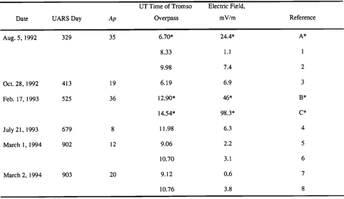
Table 1 shows the UT time of the WINDII wind altitude

profile above Tromso

for each of these 6 days. It

corresponds

to the mean

time

between

the two field of view

overpasses.

In each

case

we have

chosen

the EISCAT

data

at the closest time available. The magnetic index Ap is also

provided

in the table, as well as the electric

field value

measured by EISCAT at the times of WINDII passes. One can see that 2 days, August, 5, 1992 and February, 17, 1993, are active days but only three profiles (referenced by a letter in the table and in the following figures) locally

correspond

to periods

of large electric

fields.

For the eight

other

wind profiles

(referenced

by a number)

the magnetic

local conditions were extremely quiet with electric field amplitudes smaller than 8 mV/m.

2.1. EISCAT-Derived Meridional Winds

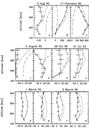
Figure 1 shows

as a solid line the meridional

wind Un

calculated from EISCAT data for each of the WINDII

overpasses:

Un= -Vi / cosI + Vdiff tan I + Uz tan I (1)

where Vi is the parallel ion velocity, Vdiff is the diffusion velocity, Uz is the vertical neutral wind, and I is the magnetic dip angle (1=68.6 ø for our data). Given the small declination angle of the magnetic field line over EISCAT (less than 1 o in the thermosphere), this wind calculated in the magnetic meridian is closely equivalent to that obtained in the geographic north-south direction from WINDII.

The dashed line shows the contribution of the ion

velocity (-Vi / cosI ), and the dashed-dotted line shows the

contribution of the diffusion velocity (-Vdiff tan I). It has

been assumed that the vertical neutral wind was zero. As

one can see in Figure 1, the diffusion velocity plays a major role with amplitudes at 250 km altitude ranging between about 30 m/s (profile A) and 100 m/s (profile 3). It is consequently important to point out here the main

uncertainties in its calculation. The altitude variation of

Vdiff is mainly due to the gradients of the electron density: for example one can compare profiles obtained on August,

Table 1. WINDII - EISCAT Correlative Experiments

Date UARS Day Ap

UT Time of Tromso Overpass Aug. 5, 1992 329 35 6.70* 8.33 9.98

Oct.

28, 1992

413

19

6.19

LATHUILLERE ET AL.' EISCAT-WINDII THERMOSPHERIC WINDS 4489 5 Aug 92 17 February 93

I / , ! o \

150

-100 0 0 200 400 0 100 200 300

5 August 92 28 Oct 92 21 Jul 93

,,

!

//'

150 •'"• ....

-50 0 50 100 -50 0 50 100 -50 0 50 100 -50 0 50 100

1 March 94 2 March 94

I'"' I'",LI"•'/I .... I .... I1'"• .... 1•" ' I .... II .... I,'¾u' I .... I .... II .... IX•'I .... I ....

T2'

-

-

•,

,

•

• ,, -

Figure 1. Profiles of the EISCAT calculated meridional winds (solid line), which correspond to the differences

between the projection of the measured ion velocity (dashed line) and the projection of the diffusion velocity (dashed-

dotted line). The Burnside factor has not been used here.

The letters and numbers refer to Table 1.

5, 1992

(profiles

1 and

2), for which

the

maximum

electron

density occurs above 320 km altitude, with profiles obtained in March 1994 (profiles 4 to 8), when the maximum of the

F layer is around 250 km.

The amplitude of Vdiff is inversely proportional to the

ion-neutral collision frequency, which at the altitudes that

we consider is primarily the O'O collision frequency (see

Lilenste n and Lathuillgre [ 1995] for the explicit formulation

of the ambipolar diffusion velocity that we have used here). The neutral densities used in collision frequency calculations have been obtained from the MSIS-90 model for the given date and time, with the Ap indices of Table 1 and an exospheric temperature equal to the measured ion temperature at 280 km altitude. This procedure may overestimate the neutral temperature in the case of Joule

heating and consequently overestimate the neutral densities. That is why the exospheric temperature has in addition been

limited to 1200 K. Furthermore, we have used two differe nt

formulations

of the O'O collision

frequency:

(1) the value

proposed by Salah [1993] as a recommended interim consensus standard value, which includes the so-called

Burnside factor of 1.7 proposed to reconcile the ground

interferometer data and the radar data [Burnside et al., 1987], and (2) the same value without this 1.7 factor.

The diffusion velocity shown in Figure 1 corresponds to

the second value, i.e., without the Burnside factor. It

emphasizes the importance of the contribution of the

diffusion velocity in the calculation of the meridional wind.

Using the Burnside factor will reduce the diffusion velocity

by a factor of 1.7.

2.2. Comparison of WINDII and EISCAT Winds In Figure 2 we show in solid lines the meridional wind measured by WINDII. These values use the zero wind

reference described by Gault et al. [1996].

Results of EISCAT calculations are shown as dashed- dotted lines when the Burnside factor is included in the O+O

collision frequency and as dotted lines when the Burnside

factor is not used. The error bars have not been plotted in this figure for more clarity, but they are given in Figure 1. Two different behaviors are clearly seen in Figure 2: for the first three profiles referenced by a letter there is obviously

little agreement between the two instruments. The EISCAT-

WINDII wind differences are of the order of 100 m/s. As

was noted above, these three profiles correspond to active periods according to the electric field values of Table 1. Under these conditions our assumption of zero vertical

3OO 250 200 150 -200 -100 5 Aug 92 17 February 93 '1 .... 'l'.•"k.' ' I I ... '''' ,,, :1-' ' :IF

,,/

',, /'

/'

5 August 92 28 Oct 92 21 Jul 93 300 25O 2OO 150 -50 0 50 -50 0 50 -50 0 50 -50 0 50 1 March 94 2 March 94 25O 2OO 150 -50 0 50 -50 0 50 -50 0 50 -50 0 50 Meridional Wind [m/s]

Figure 2. Comparison

of the meridional

wind profiles

measured by WINDII (solid line) and those calculated by

EISCAT. The dashed-dotted line is obtained when the

Burnside factor is included in the O + O collision frequency,

4490 LATHUILLERE ET AL.: EISCAT-WINDII THERMOSPHERIC WINDS

winds is certainly not valid. Because of the factor tan I in equation (1) a vertical upward wind of about 25 m/s could explain the differences. Much larger vertical neutral winds have already been observed in auroral zones during active periods. Indeed, Fauliot et al. [1993] have been able to give an empirical formulation to relate the vertical wind measured by the MICADO instrument to the local variation of the magnetic field.

Vertical winds, however, are not the only problem in EISCAT calculations. These periods also correspond to strong Joule heating: neutral temperature and densities may be quite different from the one obtained from MSIS-90.

On the other hand, WINDII apparent quantities have been inverted under the assumption of a locally spherically isotropic and time invariant atmosphere [Gault et al., 1996]. It is likely that in the cases of large gradients, as can be found in the auroral thermosphere, the result of the inversion will represent a mean value along the WINDII line of sight. In such cases it might be more appropriate to use tomographic methods with constraints to invert the WINDII data, methods that would take into account a latitudinal variation of the winds along the line of sight.

Such a variation is already present in the corresponding

zonal winds observed by WINDII on February 17 (not shown here) that are of the order of-600 m/s over the latitudinal range 60 ø to 70 ø .

The eight profiles referenced by a number have been

plotted with the same scale. For them the overall agreement is very good. Only profile 2 displays a clear difference

between the two instruments for both calculations of the

diffusion velocity. One can also observe that the good

agreement usually breaks down at the lowest altitude of EISCAT measurements, i.e., 168.5 km. At this altitude the

contribution of the diffusion velocity is very small: indeed,

the mean difference between the meridional wind measured

by WINDII with the green line and the EISCAT-calculated

wind, neglecting the diffusion velocity, was less than 5 m/s

[Gault

et al., 1996]. On the other

hand

the O(tD) emission

-50 0 5O find l)ifference [m/s]

300

i

/

Figure 3. Histograms of (left) the differences between WINDII and EISCAT meridional winds and (right) mean differences as a function of altitude. The upper left panel and the solid line correspond to EISCAT-calculated winds that do not include the Burnside factor. The lower left panel and the dashed line correspond to EISCAT•calculated

winds that include the Burnside factor.

is much weaker at this altitude than above, and measured winds may be more sensitive to the inversion method used. More work is necessary to understand these differences.

Looking more carefully at the eight profiles, we generally find a better agreement between WINDII winds and the

EISCAT-calculated ones when the Burnside factor is not

used. This is not the case for the two profiles of August 5, 1992 (profiles 1 and 2). These two profiles correspond to a quiet period that just follows an active one (see Table 1). Indeed the ion velocity diffusion does not show a maximum because of a particularly high F layer. It is likely that perturbations of neutral densities are still present at these times, making it very difficult to obtain a correct estimate of the diffusion velocity.

3. Discussion

The WINDII meridional winds have been interpolated at the altitudes of EISCAT observations excluding the lowest one, and wind differences have been calculated (WINDII wind versus EISCAT wind). Histograms of these differences are presented in the two left panels of Figure 3. One shows the wind differences when the diffusion velocity is calculated without the Burnside factor (upper panel), and the other shows them with the Burnside factor (lower panel). The mean values are +5.5 m/s and-8 m/s, respectively, and the standard deviation is 18.6 m/s and 21.6 m/s. The panel on the right shows the mean differences as a function of the altitude with values greater than 2 sigma removed. At 190 km altitude, both values are positive and close to each other because the diffusion velocity is very

small. These values are close to the mean difference that has

previously

been found between

EISCAT and O(•S)

meridional winds, as noted in the previous section. At

higher altitudes there is a consistent positive bias between WINDII and EISCAT if the Burnside factor is not used and

a negative one in the other case.

Whatever the choice of the ion - collision frequency values, our comparisons allow us to conclude that the

EISCAT measurements confirm the WINDII zero wind

reference

for the O(tD) emission

within 10 m/s. This was

also

the

conclusion

of the

validation

of O(tS)

winds

against

external measurements [Gault et al., 1996].

Can we make any conclusive statement about the value of

the Burnside factor?

First, our aim here was not to try to obtain this factor, as

was done in previous work. This process would require more coordinated measurements to obtain meaningful statistics and a more precise WINDII zero wind calibration validated against more external measurements.

Nevertheless, several arguments make us think that our EISCAT-derived winds are in better agreement with

WINDII measurements when the Burnside factor is not

included

in the O+O collision

frequency:

(1) Figure

2 shows

that there were more profiles in good agreement in this case; (2) the form of the histogram of the WINDII-EISCAT differences (Figure 3) is closer to a Gaussian; and (3) the mean wind difference is slightly positive (Figure 3), as were

most

of the wind

differences

found

between

O(•S) WINDII

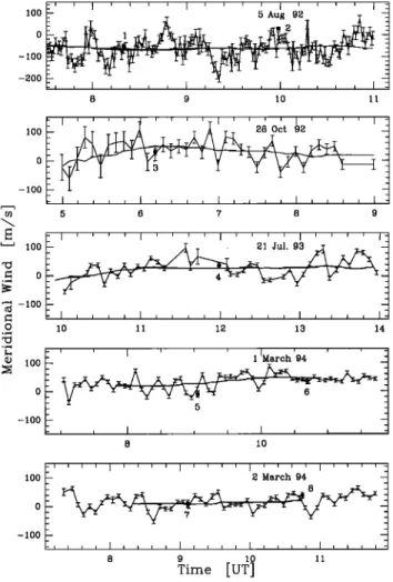
winds and external measurements [Gault et al., 1996]. In Figure 4 we show examples of the time variations of the EISCAT meridional winds at 256 or 234 km altitude, calculated without the Burnside factor, for the five quiet

LATHUILLERE ET AL.: EISCAT-WINDII THERMOSPHERIC WINDS 4491 100 •-- 5 Aug. 92 0 1 _•l•mT_ _T -200 8 9 10 11 100 •T . I . i . 28 Oct. 92 -100 • 5 6 7 8 9 • -100 • . 0 10 11 1• 13 14

• 100

'

I

'

'

'

1 [March

'94 '

'

o

Figure 4. Time variations of the EISCAT meridional wind for the quiet periods at 234 km altitude (March 1, 1994) or 256 km ( 4 other days). The smooth line is a 2-hour running average. The WINDII wind values are superimposed and marked by the reference numbers of Table 1.

periods, on which the WINDII winds are superimposed. The numbers indicated on each panel are the profile

reference numbers from Table 1. When the EISCAT

integration time was 5 min (three lower panels), the EISCAT timescale was shifted by + 2.5 min, in order to

attribute the EISCAT wind to the mean time of the

integration period. The WINDII time corresponds to the mean value between two very short measurements taken 8

min apart. This comparison is the best one that can be

achieved in terms of temporal resolution for our two sets of data. The smooth line superimposed on each panel is a 2

hour running average of the EISCAT winds. One can see that the WINDII winds agree with the 1 min or 5 min

integrated EISCAT winds in all the experiments and disagree with the means when they are far from the instantaneous measurements (point 2 on August 5 and 5 on

March 1). More examples exist at different altitudes, but it

does not seem necessary to show them as graphs.

Indeed we have first tried to make the comparison between WINDII data and EISCAT profiles averaged over 2 hours. This was done in order to damp down the observed oscillations in EISCAT data. The agreement was worse, as can be seen in the two examples shown in Figure 4.

4. Conclusion

We have here shown the first comparison between altitude profiles of meridional winds obtained by two completely different methods. The excellent agreement found in the case of quiet local magnetic conditions gives us

confidence that both data sets are correct within 10 m/s.

When electric fields are present in the ionosphere, large discrepancies are found; these can be explained by the

intrinsic

limitations

6f the two techniques

used

to obtain

meridional wind measurements.

We have found that our two sets of data were in better

agreement when the Burnside factor was not included in the

O+O collision frequency calculation. However, as we have

pointed out, this result has to be validated by using other data. This can be done by using the midlatitude and low-

latitude incoherent scatter radar data that are correlated to

WINDII O(•D) measurements.

Finally, we have found a better agreement between EISCAT and WINDII wind profiles without any temporal averaging of data, suggesting that the oscillations found in

the EISCAT-calculated meridional winds are real

oscillations of the neutral atmosphere that are present even in the case of very low magnetic activity.

Acknowledgements. The WINDII project is sponsored by the Canadian Space Agency and the Centre National d'Etudes Spatiales. EISCAT correlative investigations have been supported by the Centre National de la Recherche Scientifique (program PAMOY). The EISCAT facility is supported by the research councils of Finland (SA), France (CNRS), the Federal Republic of Germany (MPG), Norway (NAVF), Sweden (NFR) and the United Kingdom (SERC). Part of the calculation have been made

in the Centre de Calcul Intensif de l'Observatoire de Grenoble.

The editor thanks Joseph E. Salah and another referee for their assistance in evaluating this paper.

References

Bourg, L., Contribution h l'•tude de la dynamique de la m•sosph•re: Interpretation des mesures de l'interf•rom•tre WINDII plac• h bord du satellite UARS, th•se de doctorat,

Univ. Paris 7, 1995.

Burnside, R.G., C.A. Tepley, and V.B. Wick. war, The O+-O

collision cross section: Can it be inferred from aeronomical

measurements?, Ann. Geophys., Ser.5A., 343-350, 1987.

Fauliot, V., G. Thuillier, and M. Hers•, Observation of the F-

region horizontal and vertical winds in the auroral zone, Ann. Geophys., 11, 17-28, 1993.

Gault W.A., et al., Validation of O(tS) wind measurements by

WINDII: The wind imaging interferometer on UARS, J. Geophys. Res., 101, 10, 405-10, 430, 1996.

Lilensten, J., and C. Lathuill•re, The meridional thermospheric neutral wind measured by the EISCAT radar, J. Geomagn.

Geoelectr., 47, 911-920, 1995.

Lilensten, J., G. Thuillier, C. Lathuill•re, W. Kofman, V. Fauliot, and M. Herse, EISCAT-MICADO coordinated measurements

of meridional wind, Ann. Geophys., 1 O, 603-618, 1992. McLandress, C., Y. Rochon, G.G. Shepherd, B.H. Solheim, G.

Thuillier, and F. Vial, The meridional wind component of the thermospheric tide observed by WINDII on UARS, Geophys.

Res. Lett., 21, 2417-2420, 1994

Salah, J.E., Interim standard for the ion-neutral atomic oxygen collision frequency, Geophys. Res. Lett., 20, 1543-1546, 1993. Shepherd, G.G., et al., WINDII: The wind imaging interferometer

on the Upper Atmosphere Research Satellite, J. Geophys. Res.,

98, 10,725-10,750, 1993a.

Shepherd G.G., et al., Longitudinal structure in atomic oxygen concentration observed with WINDII on UARS, Geophys. Res.

Lett., 20, 1303-1306, 1993b.

4492 LATHUILLERE ET AL.: EISCAT-WINDII THERMOSPHERiC WINDS

influence on O(1S) airglow emission rate distributions at the

geographic equator as observed by WINDII, Geophys. Res.

Lett., 22,275-278, 1995.

Thuillier,

G., and

M. Hers&

Thermally

stable

field

compensated

Michelson interferometer for measurement of tempe?ature and wind of the planetary atmospheres, Appl. Opt., 30, 1210-1220,

1991.

Thuillier, G., V. Fauliot, M. He rs& L. Bourg, and G.G. Shepherd,

The MICADO wind measurements from Observatoire de

Haute-Provence for the validation of the WINDII green line data, J. Geophys. Res., 101, 10, 431-10, 440, 1996.

C. Lathuill•re and J. Lilensten, Centre d'Etudes des

Ph6nom•nes A16atoires et G6ophysiques, Ecole Nationale Superieure des Ing6nieurs Electriciens de Grenoble, B. P. 46, 38402 St Martin d'H•reg, France.(e-mail' chantal@cephag.observ- gr.fr)

G. Thuillier, Service d'A6ronomie, Centre NatiOnal de la

Recherche Scientifique, B. P. 91371 Verri•res le Buisson, France

W. Gault, York University, Toronto, Ontario, Canada,

M3J1P3.

(Received June 3, 1996; revised October 21, 1996;