Cycle-to-cycle control of multiple input-multiple output manufacturing processes

(1)

Cycle-to-Cycle Control of Multiple Input-Multiple Output Manufacturing Processes

by

Adam Kamil Rzepniewski

B.S., Mechanical Engineering University of Notre Dame, 1999

S.M., Mechanical Engineering

Massachusetts Institute of Technology, 2001 Submitted to the Department of Mechanical Engineering in Partial Fulfillment of the Requirements for the Degree of

Doctor of Philosophy in Mechanical Engineering at the

Massachusetts Institute of Technology

June 2005

Signature redacted

Signature of Author . .re

S

nu.

.acted

Departme of Mechanical Engineering

May 5, 2005

Signature redacted

Certified by ... ...

David E. Hardt Professor of Mechanical Engineering

Signature redacted

Thesis Supervisor

Accepted by... ...

Lallit Anand Chairman, Department Committee on Graduate Students

MASSACHUW SETTU OF TECHNOLOGY

JUN

1 2005

S6

(2)

MITLibraries

Document Services Room 14-0551 77 Massachusetts Avenue Cambridge, MA 02139 Ph: 617.253.2800 Email: docs@mit.edu http://libraries.mit.edu/docs

DISCLAIMER OF QUALITY

Due to the condition of the original material, there are unavoidable flaws in this reproduction. We have made every effort possible to provide you with the best copy available. If you are dissatisfied with this product and find it unusable, please contact Document Services as soon as possible.

Thank you.

The images contained in this document are of

the best quality available.

(3)

Cycle-to-Cycle Control of Multiple Input-Multiple Output Manufacturing Processes

By

Adam Kamil Rzepniewski

Submitted to the Department of Mechanical Engineering

on May 5, 2005 in Partial Fulfillment of the Requirements for the Degree of Doctor of Philosophy in Mechanical Engineering

ABSTRACT

In-process closed-loop control of many manufacturing processes is impractical owing to the impossibility or the prohibitively high cost of placing sensors and actuators necessary for in-process control. Such processes are usually left to statistical process control methods, which only identify problems without specifying solutions. In this thesis, we look at a particular kind of manufacturing process control, cycle-to-cycle control. This type of control is similar to the better known run-by-run control. However, it is developed from a different point of view allowing easy analysis of the process' transient closed-loop behavior due to changes in the target value or to output disturbances. Both types are methods for using feedback to improve product quality for processes that are inaccessible within a single processing cycle but can be changed between cycles. Through rigorous redevelopment of the control equations, we show these methods are identical in their response to output disturbances, but different in their response to changes in the target specification.

Next, we extend these SISO results to multiple input-multiple output processes. Gain selection, stability, and process variance amplification results are developed. Then, the limitation of imperfect knowledge of the plant model is imposed. This is consistent with manufacturing environments that require minimal cost and number of tests in determining a valid process model. The effects of this limitation on system performance and stability are discussed. To minimize the number of pre-production experiments, a generic, easily calibrated model is developed for processes with a regional-type coupling between the inputs and outputs, in which one input affects a region of outputs. This model can be calibrated in just two experiments and is shown to be a good predictor of the output. However, it is determined that models for this class of process are ill-conditioned for even moderate numbers of inputs and outputs. Therefore, controller design methods that do not rely on direct plant gain inversion are sought and a representative set is selected: LQR, LQG, and H-infinity. Robust stability bounds are computed for each design and all results are experimentally verified on a 110 input-i 10 output discrete-die sheet metal forming process, showing good agreement.

Thesis Supervisor: David E. Hardt

(4)

ACKNOWLEDGMENTS

To my parents Zdzislaw and Helena Rzepniewski and Sister Eva who have patiently supported me throughout not only this venture, but all things that I have done in my life.

Thank you.

I would like to thank my advisor David E. Hardt (Dave) who has spent a considerable

amount of time in discussions with me, even when it was a Friday afternoon before a long weekend. Thank you for all of your support, you are the best advisor a student can have.

Thank you to my co-workers. Most specifically, thank you to Catherine L. Nichols who had started as a co-worker, but has become the love of my life. Thank you to Chip Vaughan and Bala Ganesan, who had made beach trips a regular event during the summer months. Thank you to Johnna Powell and Susan Brown with whom I had many conversations; some actually work related! Thank you to Benny Budiman who showed me how to graduate in style. Finally, thank you to my current co-workers Matt Dirckx, Grant Shoji, Kunal Thacker, and Wang Qi who had to put up with me during the last months of this dissertation.

(5)

FIGURES

Figure 1-1 Exam ple output distributions. ... 14

Figure 1-2 Example process distributions with specification limits; lower specification limit (LCL) and upper specification limit (USL). Centered distribution (left) and significantly non-centered distribution (right)... 15

Figure 1-3 Three types of closed-loop control... 19

Figure 1-4 Spatially coupled output diagram. A single input at point 3 affects outputs 1-5. ... _{2 1} Figure 1-5 Expanded process block diagram for CtC control. ... 23

Figure 1-6 Simplified process block diagram... 24

Figure 1-7 Process model linearization through a "small range" assumption... 25

Figure 1-8 Schematic of sheet metal stretch forming. ... 26

Figure 1-9 Manufacturing process control laboratory's stretch forming machine (left) and die surface detail (right). Die surface dimensions of 11.5 in x 12 in... 27

Figure 1-10 Reconfigurable tool produced by Northrop Grumman and Cyril Bath. The forming surface is 4 ft x 6 ft in area. (See Papazian, [], for design details)... 28

Figure 1-11 Schematic of a gross/fine pressure configuration for hot micro-embossing. 29 Figure 1-12 Schematic of a heating grid for local temperature in hot micro-embossing. 30 Figure 1-13 Deep drawing process schematic (left), Segmented binding ring (right)... 31

Figure 1-14 Robotic fixtures with sheet workpiece; car door welding example... 31

Figure 1-15 Schematic of chemical-mechanical polishing... 32

Figure 2-1 Process block diagram ... 42

Figure 2-2 z-plane stable region with constant damping and constant frequency lines, [1 0 ]... _{4 3} Figure 2-3 EWMA-based control block diagram. ... 48

Figure 2-4 Integral-based control block diagram... 48

Figure 2-5 Integral controller root locus... 50

Figure 2-6 IMA(1,1) and correlating filter (Equation 2-33) outputs with a defined by N (O ,1)... 5 2 Figure 2-7 Ratio of the variance of the process output and NIDI shocks a, when the additive noise model is described by the IMA(1,1) model... 53

Figure 2-8 Ratio of the variance of the process output and NIDI shocks a, when the additive noise model is described by the correlated noise model, Equation 2-33.... 54

Figure 2-9 Ratio of the variance of the process output and the additive noise, d. Noise described according to Equation 2-33... 55

Figure 2-10 Control space of the predictor-corrector controller. Figure reproduced from w ork by Chen and Guo, [19]... 57

Figure 2-11 Controller zero location, y, as a function of the EWMA weights for the predictor-corrector controller set of equations... 61

Figure 2-12 Controller zero location, y, as a function of the EWMA weights for the d-EW M A set of equations... 61

Figure 2-13 Double EW M A root locus. ... 63

Figure 2-14 Ratio of the variance of the process output and the additive noise, d. Noise described according to Equation 2-33, P=0.00. ... 71

(9)

Figure 2-15 Ratio of the variance of the process output and the additive noise, d. Noise described according to Equation 2-33, P=0.80. ... 71

Figure 3-1 Proportional-Integral controller diagram. ... 77

Figure 3-2 Typical SISO PI controller-CtC plant root locus (left) and corresponding unit step response (right) with the controller zero placed at z=0.5... 78 Figure 3-3 Typical SISO PI controller-CtC plant root locus (left) and corresponding unit

step response (right) with the controller zero placed at z=-0.5... 79

Figure 3-4 Selected input-output data for a plant matrix in Equation 3-20... 83 Figure 3-5 Input-output data for process in Equation 3-24 with deadbeat analog gain

selectio n . ... _{8 5} Figure 3-6 Process noise amplification for NIDI noise as a function of the norm of the

lo o p g ain ... _{8 8} Figure 3-7 Process noise amplification for correlated noise as a function of the norm of

the loop gain. MIMO correlation factor P=O.8... 89

Figure 4-1 Quarter symmetry part used in MA TLAB and ABA QUS simulations. Symmetry along the X =1 and Y=1 axes... 93

Figure 4-2 X coordinate error response as a function of closed loop run number. Gaussian function description of coupling, uncoupled controller. MATLAB simulation.

Coordinates labeled as in Figure 4-1. ... 95

Figure 4-3 Y coordinate error response as a function of closed loop run number. Gaussian function description of plant coupling, uncoupled controller. MATLAB simulation. Coordinates labeled as in Figure 4-1. ... ₉₆ Figure 4-4 X coordinate error response as a function of closed loop run number.

ABA QUS-based plant model, uncoupled controller. Coordinates labeled as in Figure

4 - 1 . ... _{9 8} Figure 4-5 Y coordinate error response as a function of closed loop run number.

ABA QUS-based plant model, uncoupled controller. Coordinates labeled as in Figure

4 - 1 . ... _{9 9} Figure 4-6 Closed-loop process poles (left) and zeros (four graphs on the right) on the

complex plane. Zero results are displayed according to their position in the process m atrix ... _{10 1} Figure 4-7 Process settling time based on 2% (left) and 0.2% (right) of target value. 5,000 to tal cou n t... ₁₀₂ Figure 4-8 Closed-loop process poles (left) and zeros (right) on the complex plane. Zero

results are displayed according to their position in the process matrix)... 102 Figure 4-9 Closed-loop process settling time based on 2% of final value. 5,000 total

c o u n t... _{10 3} Figure 4-10 Process settling time based on 2% of final value. 5,000 total count... 104 Figure 4-11 Percent of processes settling to within 2% of target in 2 time steps or fewer

as a function of pre-process plant misidentification level. Level defined as the standard deviation of additive perturbation in Equation 4-3. ... 105

Figure 4-12 Percent of processes settling to within 2% of target in two time steps or fewer as a function of during-process plant misidentification level. Level defined as the standard deviation of additive perturbation in Equation 4-6. ... 106

Figure 5-1 Gain magnitudes as a function of pin position for intermediate pin (3,3), (left), and center pin (1,1), (right)... 111

(10)

Figure 5-2 Gain spread as a function of pin position for (3,3) pin. X direction, xY= 1.5,

scale = 0.4 (left), Y direction, cy = 1.1, scale = 0.3 (right)... 111

Figure 5-3 Gain spread as a function of pin position for (1,1) pin. X direction, ax = 1.6, scale = 0.5 (left), Y direction, ayy= 1.13, scale = 0.5 (right)... 112

Figure 5-4 Uniformly scaled Gaussian spread function. ... 113

Figure 5-5 Non-uniformly scaled Gaussian spread function (a) and its scaling (b)... 114

Figure 5-6 Scaling factors shown according to their position in a IxlO grid of inputs. Uniform column scaling (a) Non-uniform column scaling (b)... 115

Figure 5-7 Five cylinder dies used for extended model testing... 117

Figure 5-8 Error between predicted and formed part. (Left) Maximum absolute error (right) Norm of part error (ABAQ US simulated forming, Noiseless conditions). .. 118

Figure 5-9 Error between predicted and formed part. (Left) Maximum absolute error (right) Norm of part error (ABAQUS simulated forming, Noisy conditions). ... 118

Figure 5-10 Error between predicted and formed part. (Left) Maximum absolute error (right) Norm of part error; smoothed plant matrix (ABAQUS simulated forming, N oisy con ditions)... 119

Figure 5-11 Pin scaling vector as a function of test number. Numbering defined in Table 5 - 1 . ... 12 0 Figure 5-12 Error between formed and predicted part. Maximum error (left), Norm of erro r (righ t)... 12 1 Figure 5-13 Matrix condition number (Frobenius Norm) as a function of the number of rows or columns in a square Gaussian matrix. Assumed coupling o= 1, no scaling is u se d . ... 12 2 Figure 6-1 General block diagram, additive uncertainty. ... 124

Figure 6-2 General block diagram, multiplicative uncertainty... 124

Figure 6-3 M ass-spring-dam per system ... 127

Figure 6-4 Uncertain m ass block diagram . ... 128

Figure 6-5 Example closed-loop process block diagram... 133

Figure 6-6 Example p bounds (Yupper and vjower) as a function of frequency. Example process is the nine input-nine output case in Example 6-5. Since this is a discrete-time process, the needed frequency range is [0,n]... 137

Figure 6-7 CtC block diagram with process uncertainty. ... 140

Figure 6-8 Feedback block diagram with output disturbance. Figure reproduced from [3 5 ]... 14 5 Figure 6-9 Feedback block diagram with performance as stability. Figure reproduced fro m [3 5 ]. ... 14 5 Figure 6-10 Feedback block diagram with mixed stability and performance. ... 146 Figure 7-1 Discrete die sheet metal forming block diagram. Figure adapted from Norfleet,

[3 0 ]... 14 9 Figure 7-2 Part support for use in coordinate measurement machine (left) and formed part (rig h t). ... 15 3

Figure 7-3 Obtained pole locations and control gains calculated via Kautsky et al. method. A lOx10 bundle of inputs (totaling 100) is assumed and the 4 5th input (occurring near the center of the bundle) is displayed. All poles are located at the o rig in ... 15 5

(11)

Figure 7-4 Obtained pole locations and control gains calculated via Kautsky et al. method. A IOx10 bundle of inputs (totaling 100) is assumed and the 4 5th input (occurring near the center of the bundle) is displayed. All poles are located within a

0.3 band on the z-plane... 156 Figure 7-5 Simulated closed-loop runs of a 110 input, 110 output process with LQR

designed integral controller gain matrix. Noiseless simulation (left) and Noisy sim ulation (right). m = 100. ... 160

Figure 7-6 pA bounds as a function of frequency for a closed loop process with an LQR designed integral controller gain matrix. m=100... 161

Figure 7-7 Simulated closed-loop runs of a 110 input, 110 output process with LQR designed integral controller gain matrix. Noiseless simulation (left) and Noisy sim ulation (right). m = 1,000. ... 162

Figure 7-8 pA bounds as a function of frequency for a closed loop process with an LQR designed integral controller gain matrix. m=1,000... 162

Figure 7-9 Experimentally obtained section of a 27cm radius cylinder. ... 163

Figure 7-10 Experimental closed-loop runs of the sheet metal forming process described in Section 1.5.1. Mean error shown, LQR designed integral controller gain matrix,

m = 10 0 . ... 164 Figure 7-11 Experimental closed-loop runs of the sheet metal forming process described

in Section 1.5.1. Maximum (based on magnitude) and RMS error shown, LQR designed integral controller gain matrix, m=100... 165

Figure 7-12 Experimental closed-loop runs of the sheet metal forming process described in Section 1.5.1. LQR designed integral controller gain matrix, m= 1,000... 166 Figure 7-13 Experimental closed-loop runs of the sheet metal forming process described

in Section 1.5.1. Maximum (based on magnitude) and RMS error shown, LQR designed integral controller gain matrix, m= 1000... 167

Figure 7-14 Representation of uncertainty in feedback control, [33]... 170

Figure 7-15 Plant description used for Kalman filter design... 172

Figure 7-16 Simulated closed-loop runs of a 110 input, 110 output process with H2 designed controller. Noiseless simulation (left) and Noisy simulation (right)... 173 Figure 7-17 pA bounds as a function of frequency for a closed loop process with an H2

designed controller... 173

Figure 7-18 H2 simulation, Kalman observer estimated output (left) and actual time response (right) with non-zero initialized observer states. ... 175

Figure 7-19 H2 simulation with registering. Kalman estimate of the output (left) and actual simulated output (right). A noiseless simulation is used... 176

Figure 7-20 Experimental closed-loop runs of the sheet metal forming process described in Section 1.5.1. H2 (LQG) designed controller... 177 Figure 7-21 Experimental closed-loop runs of the sheet metal forming process described

in Section 1.5.1. Maximum (based on magnitude) and RMS error shown, H2 (LQG)

Figure 7-22 Schematic view of two frequency response functions and the difference between the optimal solution for the H2 and H, problem... 179

Figure 7-23 H , design block diagram ... 181

Figure 7-24 Simulated closed-loop runs of a 110 input, 110 output process with H" designed controller. Noiseless simulation (left) and Noisy simulation (right)... 182

(12)

Figure 7-25 pA bounds as a function of frequency for a closed loop process with an H. design ed controller... 183

Figure 7-26 Closed-loop, noiseless response of the H, controller with registration

in clu d ed ... 18 3

Figure 7-27 Experimental closed-loop runs of the sheet metal forming process described in Section 1.5.1. H , designed controller... 184 Figure 7-28 Experimental closed-loop runs of the sheet metal forming process described

in Section 1.5.1. Maximum (based on magnitude) and RMS error shown, H.

Figure 8-1 SCA algorithm experimental application results, [2]... 187

Figure 8-2 pA bounds as a function of frequency for a closed loop process with an SCA designed controller... 188

Figure 8-3 Saddle target shape from Valjavec, [44]... 190

Figure 8-4 Diagonal scaling matrix entries shown according to their position in a lOx 1 grid of inputs. Cylinder scaling (left), saddle scaling (right)... 190

Figure 8-5 Percent deviation of each scaling value between the cylinder- and saddle-calibrated plant m atrices. ... 191

Figure 8-6 Process response plots with a saddle-configured plant matrix and cylinder-configured controller m atrices... 192

Figure 8-7 Example input-output response characteristics used to illustrate adaptive co n tro l. ... 19 8

Figure B-1 Controllable wavelength limit for a discrete-die forming machine... 204 Figure B-2 Target parts. Full frequency (left) Limited frequency (right)... 205 Figure B-3 Difference between the full-frequency and frequency-limited parts... 205 Figure B-4 Maximum error magnitude between a full-frequency and frequency-limited

part. Parts ranging from 6.65in (#1) to 14.65in (#5) radius, in 2in increments... 206 Figure C-I Plant and LQR control gains for different values of the coupling spread o. A

lOx]0 bundle of inputs (totaling 100) is assumed and the 45th input (occurring near the center of the bundle) is displayed. A relative weight of m=100 is chosen. ... 209 Figure C-2 Poles and maximum error for an LQR design controller. 1Ox10 bundle of

inputs and a spread of a=1.22 are assumed. A relative weight of m=100 is chosen.

... 2 1 0 Figure C-3 Poles and maximum error for an LQR design controller. IOx10 bundle of

inputs and a spread of o=1 .23 are assumed. A relative weight of m=100 is chosen.

... 2 1 0 Figure C-4 Plant and LQR control gains. A 15x15 bundle of inputs (totaling 225) is

assumed and the 1 0 5th row is displayed (equivalent center position of the _{4 5}th input presented in Figure C-1). A relative weight of m=100 is chosen. ... 210 Figure D- 1 Experimental process stretch distance computation. Included are results from

a fine grid (computed from only the rightmost two points) and coarse grid

(computed at each of the ten pin positions) estimation. (1) First die, (2) Second die,

(3) Third die, SCA algorithm, (4) Third die, GIC algorithm... 212 Figure D-2 Part Error for third die with fine grid suggested stretch distance (left) and

(13)

TABLES

Table 2-1 Expected process performance as a function of loop gain, kpk, for an integral

C tC controller... . . 50

Table 2-2 Expected process performance as a function of process mismatch given EWMA weights. PCC updating equations used. Results reproduced from Del Castillo, [20]. The lower boundary of region 5 is incorrect; the corrected equation is presented in Equation 2-54 and Equation 2-55... 58

Table 2-3 Expected process performance as a function of loop gain, K, and controller zero position , . ... . 65

Table 2-4 Closed-loop process responses to a target reference input (top) and disturbance input (bottom). Each response is considered independently... 69

Table 3-1 Input-output data for a prime-number state matrix. ... 82

Table 3-2 Input-Output data for the process in Equation 3-20 with deadbeat analog gain selectio n . ... 8 5 Table 3-3 Input-output data for the process in Equation 3-24 with deadbeat analog gain se lectio n . ... 8 5 Table 5-1 Standard test numbering convention for extended model testing. ... 117

Table 5-2 Standard test numbering convention for universal model testing. ... 121

Table 6-1 Small gain theorem and p-analysis bound comparison for uncertainty in the p lan t m atrix . ... 14 1 Table 6-2 p analysis bound for uncertainty in the plant matrix... 143

Table 7-1 Experiment parameters for the discrete-die sheet metal forming process discussed in Section 1.5.1... 149

Table 7-2 Kalman filter design standard deviation scaling factors... 172

T able 7-3 H , design param eters. ... 181

Table E- 1 LQR controller (m=100) experimental data... 214

Table E-2 LQR controller (m=1000) experimental data... 214

Table E-3 LQG/H2 controller experimental data. ... 215

(14)

CHAPTER

INTRODUCTION

The world of manufacturing has changed a lot since its beginnings. Production has gone from hand-manufactured parts, to machine manufactured parts for non-standardized assemblies, to part standardization and computer numerical control (CNC). In this thesis, we focus on a key technology within manufacturing that has emerged as a result of these changes: the application of feedback, or closed-loop, control to improve process output. The manufacturing control field continues to evolve as more sophisticated methods are developed and feedback is introduced at different points within the manufacturing cycle.

1.1 The Need for Control

The need for control has its roots in uncertainty. We simply do not know all of the input-output causal relations that exist both within and around the process. For example, a typical process may be subject to imprecise knowledge about the process itself or to outside disturbances such as vibration or temperature variations. It is true that one tries to minimize the disturbances either through advanced design, good knowledge of the process, or through control of the environment. However, the extent to which this can be accomplished is limited. For instance, a "true" model of a process is impractical, and usually impossible, and not all outside noise can be eliminated. This is especially true in

(15)

manufacturing environments where variations in workpiece properties are themselves a source of noise. As a result, process models are usually educated guesses and process outputs are generally described as distributions rather than point values. This is shown in Figure 1-1 where the output probability density is displayed as a function of deviation from target. As will be shown in subsequent chapters, control allows an operator to change these process distributions even in the face of uncertainty.

0.5--- --- ,-- ----

,---Normal

04

Distribution

W0.3

Uniform

Distribution 0 CL

o

iL -4 -2 0 2 4

Deviation from target

Figure 1-1 Example output distributions.

Simply changing a process is not enough; one must have a way of quantifying the benefits or drawbacks of the result. Measures of evaluating the goodness of a process, based on the idea of output distributions, have been developed by previous researchers,

[1]. Here, we will discuss three of the most common: process capabilities C, and Crk, and the expected loss function E[L(x)]. Process capabilities are defined as:

C,

-USL - LSL

(16)

Cpk USL - x x - LSL

3a- 3a

-Equation 1-2

where USL and LSL are the upper and lower specification limits, respectively, Y is the mean value of the output, and o is its standard deviation. Note that a Gaussian (normal) output distribution has been assumed in both cases.

One can immediately notice the difference between these two measures. C, focuses solely on the spread of the output, as compared to the specification limits, while Cpk

penalizes both spread and non-centering of the output between the specification limits. This may lead to two different measures of goodness for the same distribution. As an example, consider two cases as shown in Figure 1-2. Both of these have unity standard deviation with specification limits at -3 and 3. However, they have very different mean values. In fact, the process on the right has 50% of its output outside the specification limits. C, is unity for both while Cpk is dramatically affected by the difference between the two processes (unity for the left and zero for the right). Thus, both standard deviation and mean value should be considered when assessing the goodness of a process.

CP~4Cl 0.4 Cpk 1 mean=0 04 Cpk=0 mean=3 0.3 .0.3 00 0.1*0.1: LSL USL -3 -2 -1 0 1 2 3 -2 0 2 4 6

LSL Deviation from target USL Deviation from target

Figure 1-2 Example process distributions with specification limits; lower specification limit (LCL) and upper specification limit (USL). Centered distribution (left) and significantly non-centered distribution (right).

(17)

Expected loss is defined as [1]:

E[L(x)] = JL(x)f(x)dx

Equation 1-3

where L(x) is the loss function andj(x) is the probability density function for the output, x. If a Gaussian probability distribution is assumed and L(x) is a quadratic in the form of

L(x)= k(x - T)2

Equation 1-4

where k is the loss coefficient and T is the target value, then the expected loss is calculated as:

E[L(x)]=

k[+2

+(Y-T)2

Equation 1-5

Thus the expected loss function accounts for both the standard deviation and the mean of the output, as did Cpk. However, E[L(x)] has two advantages over Cpk. First, it uses the coefficient k and the quality loss function to directly translate process statistics into something tangible, such as cost. Second, the expected loss remains continuous over the entire range of outputs, x. This continuity makes the expected loss function the best for comparing processes or calculating an optimum blend of mean shift and variance change.

We have stated, without proof, that control can change the process output distribution. We have also listed three performance metrics each with its benefits. However, we have not yet highlighted the real advantage of feedback: predictability. Rather than a haphazard approach to changing the process and post-calculating the improvement or detriment, closed-loop control gives a priori predictable results. Therefore, an operator can design a control law, or input recipe alteration routine, and have a good idea of what the result will be before applying it on a physical process. This ability is especially

(18)

important in manufacturing environments where the penalty for mistakes is usually monetary.

Uncertainty will, of course, still play a part. Models used in the control design process do not perfectly reflect reality and outside disturbances continue to exist. However, deviations in the model reflect themselves as changes in performance, the sensitivity to which can be minimized, and outside disturbance rejection is an explicit part of any good controller design process. Thus, when we consider the manufacturing environment with its performance metrics, the goal or motivation for applying control can be stated as: process improvement through mean centering on target and a reduction of the process

output distribution. Expressed in terms of each performance function, the goals are to: max(C,) Equation 1-6 and/or max(Cpk) Equation 1-7 and/or min(E[L(x)]) Equation 1-8

1.2 Manufacturing Process Control: Control Methods

The work in this section has been largely presented in Rzepniewski, Hardt, and Vaughan, [2].

Because a number of control methods exist, we look at a representative set with an eye as to their drawbacks and benefits. The most widely used form of process control is statistical process control (SPC). Pioneered by Shewhart [3], the goal of this approach is to eliminate all sources of assignable causes. Assignable causes are those variations that

(19)

have a clear, or assignable, source and can therefore be eliminated. For example, a new operator changing the machine settings at a shift change is a source of variation that is easily eliminated through the use of standard operating procedures (SOP's). Once removed, the process is left only with those sources of random variation that cannot be assigned or removed. Thus, by definition, the process is at its minimum variation state. This state is called "in-control."

SPC is an open loop control method and is typified by run charts, X-bar charts, and S

charts that an operator uses to confirm that the process is behaving like a stationary, random process. Although valuable as a process-monitoring tool, SPC methods do not propose a corrective course of action; it is often left to the factory worker or process engineer to find out what to do once an "out of control" signal has been registered on a control chart. Thus, they have no true "controller."

The second level of control is evolutionary operation (EVOP), [4]. This approach is a mix of design of experiments (DOE) and on-line optimization. An experimentally determined process model is continually adjusted and re-evaluated based on incoming data. The newest model is then used to identify the best operating point. Although promising in theory, the EVOP method is practically limited to three variables due to the geometrically growing number of experiments needed to update the models of larger processes, [4].

The final level of control is closed-loop control. This control method involves an a priori, explicit process model which is used to design a controller. The designer chooses

a controller that gives the desired time response and stability properties for the closed-loop process. Stability is an important consideration since models are approximate and,

(20)

thus, do not perfectly reflect the true process. Three types of closed-loop control typically appear in manufacturing processes, as shown in Figure 1-3. Each type involves the process controller, but uses different feedback data.

Product

Specs Dimensions

CO NTR EQUIPMENT MATERIAL

Equipment Lf.AOOp

NMaterial Loop

Process Output LAoop

Figure 1-3 Three types of closed-loop control.

The first type, and the most common, involves the equipment loop. Here, the

manufacturing machine is controlled to provide consistent (deterministic) energy states to

the material. A typical example is a CNC machine. Here, the actuators are precisely

controlled to produce a desired machine motion. Unfortunately, although the machine is aware of its own states, it does not have any information about the material states or properties. Thus, it cannot adjust its own state, e.g. the tool position of the CNC machine, to respond to varying conditions and workpiece states or properties, e.g. tool wear, material stiffness, etc.

The second type of closed-loop control involves the material loop. Here, the material states are fed back and this information is then used to infer things about the process output. Potential candidates for material loop feedback include material stress, strain, or temperature. For the CNC example, one could feed back the stress state of the workpiece through measurement of the tool force. This type of feedback, although potentially very useful, is rarely used owing to the difficulty and expense of obtaining and responding to data.

(21)

The final type of closed-loop control is process output control. This type is distinguished from material loop control by the direct feedback of the desired outputs, i.e. no inferences are needed. For the CNC example, this means a direct feedback of output geometry. Once again, this type of control is rarely used because of the cost and difficulty of its application. It is important to note that the three types of closed-loop control are not exclusive of each other and should be used together to produce the best output.

Out of the methods presented, closed-loop control is the most proactive and allows the user to predict and set the behavior characteristics of a process. It is also clear that anything other than output control neglects to consider process disturbances that occur outside the equipment and material loops. Thus, we will use this type of feedback control.

1.3 Problem Constraints

Having stated a general goal for control in manufacturing and defined our choice of control, we will begin to define our problem by imposing a few constraints. Our first constraint will be placed on the frequency of sensing and control action. We will assume that we can measure and change inputs only after a process cycle is over. This limitation may stem from the prohibitively high cost or the impossibility of sensing and actuating during the process cycle itself. This limitation is especially relevant for processes in which a particular part during manufacturing is different from itself after manufacturing. As an example, consider injection molding where a "hot" part (during manufacturing) will shrink as it is cooled and prepared for use (after manufacturing). In this case, assuming poor predictability of the shrinking behavior, dimension measurements during the process are not useful. Even if we assume good knowledge of shrinking behavior, placing actuators to take action based on this knowledge is difficult and expensive.

(22)

Control applied in this manner is called cycle-to-cycle (CtC) or run-by-run (RbR), the difference between these is the subject of Chapter 2.

The second constraint is on the problem form: we will concentrate on addressing the particular problems associated with Multiple Input-Multiple Output (MIMO) CtC processes. This is not because Single Input-Single Output (SISO) problems are uninteresting, but rather because SISO CtC and RbR processes have already received a lot of attention [5, 6, 7, 8, 9]. As part of this second constraint, we will narrow our MIMO

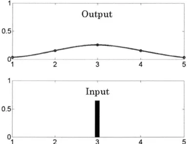
outlook to processes with "spatial-type," limited coupling such that a single input influences a finite region of outputs. A 2-dimensional example of this is shown in Figure 1-4. Here, as single input, #3, affects all outputs, #1, #2, #3, #4, and #5. We also see that the magnitude of the influence decreases with increasing distance.

1 Output 0.5 1 2 3 4 5 Input 0 L 1 2 3 4 5

Figure 1-4 Spatially coupled output diagram. A single input at point 3 affects outputs 1-5.

Our last problem constraint has a manufacturing-inspired motivation: the process should require little calibration and should provide good, stable performance. Since we are working in a manufacturing environment, each piece of "data" is potentially a

(23)

product. Therefore, any pieces that are out of specification while we are trying to configure our controller or determine our process model, cost us in terms of lost time, lost materials, and lost profits. The requirement for good, stable performance is obvious. However, we will add that fast transient response (achieving process goals with very few runs or cycles) is desirable for parts with low-production numbers, e.g. job-shop environments, which have to cope with both outside disturbances as well as changing target specifications.

1.4 The CtC Control Problem

With our choice of type of control and a number of problem-defining constraints, we finally determine our CtC problem. Specifically, we look at the block diagram of our closed-loop process and the form of all CtC plant models, regardless of particular application.

1.4.1 The CtC Control Loop

Typically, processes include multiple control loops. These loops can be independent of each other or nested inside of other loops. For example, independent actuators in a CNC machine, with their independent controllers, each may be a part of a large motion coordination controller. Because we are using process output control, we will encounter both independent and nested controllers. Figure 1-5 shows a block diagram of such a configuration. Here, we see that "machine controllers and actuators" are a part of a larger "controller." Figure 1-5 also shows that all outside influences, such as temperature variations, are modeled here as output-additive disturbances.

(24)

Controller Machine Controllers & Actuators Refeirenc -Controller Disturbances -True" -L* Plant + Noise Measured Output Figure 1-5 Expanded process block diagram for CtC control.

Although Figure 1-5 is a good depiction of reality, it remains quite complex. We will reduce this block diagram to that shown in Figure 1-6 through two assumptions. First, the "controller" is shown to encompass everything between the reference error and the input to the plant. As is shown in Figure 1-5, this means that any machine controllers and actuators are assumed to be part of the general controller. However, we will assume that the machine controllers and actuators faithfully obey the "input reference controller's" commands, see Figure 1-5. Error in this assumption may be modeled as an output additive disturbance. Note that this "faithfulness" assumption, coupled with the cycle-to-cycle control frequency, effectively removes all machine actuator loops from our view. Therefore, whenever we refer to the controller, we are referring to the "input reference controller" in Figure 1-5 and assuming perfect command following from the "machine actuators & controllers."

Second, the original disturbance and noise signals are collapsed into a single disturbance signal with the assumption that the known process output is the "measured" output rather than the "true" output, Figure 1-5. This last assumption is reasonable when

(25)

one considers that no information exists about the "true" output; we only know the, additionally noisy, "measured" output. To our benefit, measurement noise is usually orders of magnitude lower than the measurement signal.

Disturbance

Target + + Output

Controller ... Plant

Figure 1-6 Simplified process block diagram.

1.4.2 The CtC Plant Model

We have previously defined cycle-to-cycle control as an approach in which control action takes place only between cycles. This simplification in control frequency has implications for the process model. By definition, a "cycle" is not finished until all of the dynamics have finished. As a result, with our assumed inability to observe during a cycle, the process is a black box; we know what we put in and what came out but we do not know what happened in-between. Therefore, the process dynamics are reduced to a delay element, which is required to maintain causality of the plant model. The delay element is described as 1z by use of the z-transform, [10].

Additionally, the model will contain a gain describing the mapping of input and output changes. Most processes are nonlinear when one considers the full range of inputs. This nonlinearity is problematic, however, when one tries to apply classical control theory to design and analyze controller-plant combinations. In order to linearize our plant, we make a "small deviation" assumption; we assume that control action is taken in a region near the target rather than over the whole range. The effect of this is shown in Figure 1-7. Here, we see that a linear model encompassing the full range of the input, u, can do a

(26)

poor job of approximating the true process model. However, if we limit ourselves to operating within a small range u, a linear model is typically sufficient even for a nonlinear process. The process model is

Yoperating =kpu - ) > Ay - -k, Au

Z Z

Equation 1-9 where kp is the process gain and Yoperating and Uoperating are the output and input operating

points about which we linearized. The errors resulting from our linearity assumption are

modeled as additive disturbances, Figure 1-6.

6_y True Process Model Output) V Local (Linear) Process Model Full Range Process Model

Initial Operating Input

Point Point U.

Figure 1-7 Process model linearization through a "small range" assumption.

1.5 Candidate Processes

In defining our problem and searching for ways to solve it, we have to constantly keep an eye on applicability. On the one hand, we want to address specific problems and prove them experimentally on physical processes. On the other hand, we have to remain general

6 U

ell

(27)

enough to stay relevant to more than just one or two processes. In this section, we give eight examples of processes that lend themselves to cycle-to-cycle control and exhibit regional coupling, and can therefore benefit from the work presented in this thesis. We begin with a process that will become our experimental platform.

1.5.1 Discrete-Die Sheet Metal Forming

The work that led to this thesis was initially started as a short-term project to analyze a process which has existed within MIT's Manufacturing Process Control Laboratory (MPCL) for many years: discrete-die sheet metal stretch forming, [11]. Traditionally, stretch forming involves applying a stretch force to a workpiece and wrapping it around a monolithic forming tool, or die. A schematic of a stretch forming process is shown in Figure 1-8. A unique concept behind discrete-die stretch forming is dividing the traditionally monolithic forming die into many independent segments. These segments can then be rearranged between forming cycles to discretely approximate new target shapes or to eliminate disturbances.

Workpiece

Stretch Stretch

Force Force

Stretch

Force Die Movement Stretch

Force

Forming Tool (Die)

(28)

Photos of MPCL's discrete-die sheet metal forming machine are shown in Figure 1-9. This laboratory-scale process has 24 rows and 23 columns of "pins" which make up the die. Thus the process has divided the monolithic die input into 552 inputs. Although all of these inputs can be used, only 10 rows by 11 columns of pins have been used to define the region of interest for over 8 years. For comparison of results, this is the scale on which we will perform any verifying experiments. A pre-production version of this reconfigurable tooling is shown in Figure 1-10.

The discrete-die sheet metal forming CtC problem may be defined as follows. The outputs are the locus of points which make up the final shape of a sheet metal workpiece. For ease of application, we will only consider those output points which are co-located with the center of each die pin. The inputs are the individual pin positions. A clear, causal relationship thus exists between the inputs and outputs. Because the sheet metal is continuous, each input will affect a region of outputs, as required by the problem constraints. The process, run in a CtC fashion, reduces to a delay and a gain matrix relating individual pin positions to specific points on the output shape.

Figure 1-9 Manufacturing process control laboratory's stretch forming machine (left) and die surface detail (right). Die surface dimensions of 11.5 in x 12 in.

(29)

Figure 1-10 Reconfigurable tool produced by Northrop Grumman and Cyril Bath. The forming surface is 4 ft x 6 ft in area. (See Papazian, [12], for design details).

1.5.2 Fine Pressure Control for Hot Micro-Embossing

The idea of affecting regions of outputs may be extended to hot micro-embossing. In this process, a workpiece is heated beyond its glass transition temperature, into a "rubbery" state, and a patterned die is pressed into the softened material. The material is cooled before removal to maintain its patterned shape. Additional details may be found in de Mello, [13].

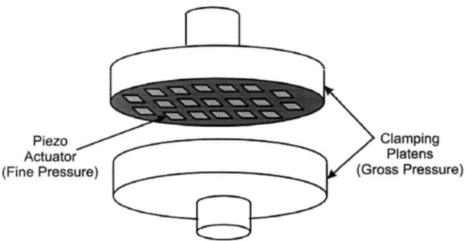
Working under the assumption that clamping pressure between the pattern and workpiece affects the final output shape, we can design a setup to vary the clamping pressure. This causal relationship assumption may be justified by performing pattern filling studies with different pressures. Rather than limiting ourselves to controlling just the gross, or overall, pressure, we want to also control the local pressure. This will allow us to compensate for changes in pattern shape or density. A schematic of such a design is

(30)

Piezo Clamping

Actuator Platens

(Fine Pressure) (Gross Pressure)

Figure 1-11 Schematic of a gross/fine pressure configuration for hot micro-embossing.

The process is thus described as follows. The outputs are the final part shapes of the workpiece. The inputs are the local pressures. Because the workpiece is not liquid, the outputs will couple according to the temporally-fixed pressure distributions from each input.

1.5.3 Temperature Control for Hot Micro-Embossing

A cause and effect relationship can also exist between the output shape and forming

temperature for hot micro-embossing. As with pressure, we want to control the local temperature to be able to compensate for changes in pattern shape or density on a single workpiece. The physical setup for controlling local temperatures is similar in concept to local pressures, as shown in Figure 1-12. Here, a grid of local heaters is used to generate the required temperature distribution over the whole workpiece.

The process has the surface profile as its output and the local heater temperatures as its inputs. The outputs are coupled through the conductivity of the workpiece.

(31)

Heating Clamping

Element Platens

Figure 1-12 Schematic of a heating grid for local temperature in hot micro-embossing.

1.5.4 Binding Pressure Control for Deep Drawing

Deep drawing is a process where a punch forces a flat workpiece into a die cavity. The process involves extensive plastic deformation as the workpiece is restrained at the edges

by the pressure between the binding ring and machine structure, as shown in Figure 1-13

(left). Common products of this process include soda cans, pots and pans. Additional details on this process may be found in Kalpakjian, [14].

An important variable in deep drawing is the binding pressure. Under- or over-application can cause wrinkling of the final product. This is especially problematic for deep drawing of non-symmetric products. An idea that fits within our problem definition and lends flexibility to the process is to divide the binding ring into independently-actuated segments, as shown in Figure 1-13 (right). The CtC process may then be defined with the extent of local thinning or wrinkling as the output and the pressure at each binding ring section as the input. The continuity of the sheet among all the inputs will couple the outputs.

(32)

Independently

Punch _Controlled

Binding Ring Sections

Workpiece

Machine

Structure

Figure 1-13 Deep drawing process schematic (left), Segmented binding ring (right). 1.5.5 Control of Robotic Fixtures for Manufacturing

Some manufacturing processes require robotic fixtures for precise positioning of the workpiece. These fixtures often over-constrain the three position and three rotational degrees of freedom, resulting in a deflection of the part. In this instance, the structure of the part will couple the effects of actuators which may be located far away from each other. This coupling can be described as spatial with more remote actuators having a lower influence on an output. As an example of this, consider the problem of spot welding a car door panel, Figure 1-14. The challenge is to locate a point of interest, the weld spot, in 3D space. Because of its size and flexibility, the workpiece requires extra support and four actuators are used. These actuators over-constrain the position of the workpiece. As such, small movements in their relative position can be used to alter the relative positions of the points of interest through deflection of the workpiece itself.

Point of Interest

Workpiece

Robotic Fixture

(33)

1.5.6 Pressure Control in Chemical-Mechanical Polishing

Chemical-mechanical polishing (CMP) is a common process in semiconductor manufacturing. The workpiece to be polished is held to a rotating pressure pad which may be used to provide both positive and negative pressure. It is then brought in contact with a rotating polishing pad which removes material from the workpiece through a combination of caustic agents and physical force. Additional details on this process may

be found in Moyne et al., [15].

The CMP process may be adopted to use the methodology contained in this thesis through a small alteration of the top pressure pad. If it is divided into sections, the top pressure pad may be used to increase or decrease the wear rate on a local area of the workpiece. The effects of different neighboring supply pressures would be coupled though the workpiece structure.

Wafer

Polishing Pad Top Pressure Pad

(34)

1.5.7 Control of Chemical Vapor Deposition

Chemical vapor deposition (CVD) is a material process. Normally, a workpiece is placed within a reaction chamber and a reactive chemical vapor is introduced. The chemical vapor then interacts with the workpiece surface such that a solid film is produced. Additional details may be found in Kalpakjian, [14]. The reactivity of the gas with the surface as well as the reaction rate are functions of the surface temperature. Therefore, if we add the ability to control the temperature locally, we will be able to control the local amount of film that is produced. Naturally, conduction within the workpiece and convection in the reaction chamber will spatially couple the outputs. The

CVD process, thus altered, can benefit from the work in this thesis.

1.5.8 Etching Control

As a final example, consider the control of wet etching. This process, as with CMP and CVD, is popular in semiconductor manufacturing. Here, the workpiece is placed in a chemical bath which selectively reacts with the surface to remove material, [14]. Because it is a chemical process, it has a notable dependence on the local concentration of reactant. Therefore, we can control the local reaction rate through the local control of concentration. To achieve this, we imagine an array of micro-pumps which can both expel as well as absorb a small amount of reactant. The effect of any single pump would be spatially distributed among the outputs (surface geometry) through diffusion within the chemical medium.

1.6 Thesis Organization

This chapter served as a brief introduction to the work we will discuss in this thesis. First, we motivated the use of feedback control to improve the output of manufacturing

(35)

processes. To do this, we showed three popular performance metrics which allow us to compare process outputs based on statistics. Additionally we stated that feedback control will allow us to predictably change those statistics. Next, we reviewed a number of control methods, focusing on output feedback closed-loop control. Then, we imposed a number of restrictions on the types of processes we wish to address. We confined ourselves only to changing control action between cycles, decided to address MIMO processes, and placed an emphasis on easy calibration of the process model and a requirement on stability in the face of uncertainty. We followed-up the constraints with a more thorough definition of the CtC control loop. Finally, we named a number of processes which can benefit from the application of cycle-to-cycle theory presented in this thesis.

The remaining chapters will build on this foundation. Chapter 2 looks at the application and the differences between SISO run-by-run and cycle-to-cycle control. Through rigorous redevelopment of the control equations, we see that the two methods address the same problem and differ in their solution only in their response to changing target specifications. These SISO results are used to develop an ideal extension of CtC control theory to multiple input-multiple output processes in Chapter 3. We conclude that we only need to know the process model to be able to design a controller. Chapter 4 looks at experimental attempts to identify the specific process model for MIMO sheet metal forming. These attempts are not successful and a simulation-based approach is taken to identifying the uncertainty tolerance of a 2x2 example MIMO process. Encouraged by the robustness results of Chapter 4, Chapter 5 presents a general, easily calibrated model which can be used on any of the processes that meet our problem constraints. We

(36)

properly account for uncertainty in Chapter 6 and present the results of applying three MIMO controllers to the sheet metal forming process, Section 1.5.1, in Chapter 7. Finally, conclusions and future work are discussed in Chapter 8.

(37)

CHAPTER

2 EWMA,

DOUBLE

EWMA

AND INTEGRAL

CONTROL

Before we can address the issues in MIMO cycle-to-cycle control, we need to understand the equations and assumptions that make up single input-single output run-by-run and cycle-to-cycle control approaches. To do this, we will look at them from the point of view of feedback control theory, focusing on time responses and errors. This is done in contrast to other views which focus on the noise transmission properties. It will become apparent that the feedback control perspective brings to light some assumptions made in the process and control equations, and reduces the number of variables to be considered.

This chapter is divided into two main sections, both concerned only with SISO control. We will not begin to consider MIMO problems until Chapter 3. The first section of this chapter addresses exponentially weighted moving average (EWMA) -based control and integral control. These controllers are meant for processes subject to little or no ramp disturbance. The second section addresses the choice of controllers for processes which are subject to a measurable drift, or ramp disturbance, considering double-EWMA and double integrator-zero controllers in particular. Although this thesis focuses mainly on the application of cycle-to-cycle control to MIMO processes with little or no drift,