HAL Id: hal-02648480
https://hal.archives-ouvertes.fr/hal-02648480
Submitted on 29 May 2020
HAL is a multi-disciplinary open access
archive for the deposit and dissemination of
sci-entific research documents, whether they are
pub-lished or not. The documents may come from
teaching and research institutions in France or
abroad, or from public or private research centers.
L’archive ouverte pluridisciplinaire HAL, est
destinée au dépôt et à la diffusion de documents
scientifiques de niveau recherche, publiés ou non,
émanant des établissements d’enseignement et de
recherche français ou étrangers, des laboratoires
publics ou privés.
Velocity distribution in open channel flow with spatially
distributed roughness
Ludovic Cassan, Hélène Roux, Denis Dartus
To cite this version:
Ludovic Cassan, Hélène Roux, Denis Dartus.
Velocity distribution in open channel flow with
spatially distributed roughness. Environmental Fluid Mechanics, Springer Verlag, 2019, pp.1-19.
�10.1007/s10652-019-09720-x�. �hal-02648480�
OATAO is an open access repository that collects the work of Toulouse
researchers and makes it freely available over the web where possible
Any correspondence concerning this service should be sent
to the repository administrator:
[email protected]
This is an author’s version published in:
http://oatao.univ-toulouse.fr/25765
To cite this version:
Cassan, Ludovic and Roux, Hélène
and Dartus, Denis
Velocity distribution in open channel flow with spatially
distributed roughness.
(2019) Environmental Fluid Mechanics.
ISSN 1567-7419.
Official URL:
https://doi.org/10.1007/s10652-019-09720-x
Velocity distribution in open channel flow with spatially
distributed roughness
Ludovic Cassan1 · Hélène Roux1 · Denis Dartus1
Abstract
A numerical procedure is proposed to estimate the velocity distribution in open channel flow, for engineering applications. A method based on the mixing length model and sub-division of the wetted surface, is modified to easily integrate a lateral distribution of rough-ness. Several friction models for vegetated or rough flows can be added, two of which have been tested. The numerical procedure was developed with a commercial software (Matlab) to ensure fast computation and possible coupling with 1D hydraulic models. The validation of the computation has been done with rectangular and compound channels with spatially distributed roughness. The usefulness of the method for ecohydraulics is demonstrated with two applications: box culvert design for fish passes and 1D modelling of mountain river flows for which experimental results from a laboratory scale-model is compared to predictions. The interest of a friction law calibrated with a real grain roughness size is put forward.
Keywords Roughness · Numerical modelling · Velocity distribution · Fish pass · Mountain river
1 Introduction
The computation of the velocity distribution in an open channel often needs a CFD method to take into account all the processes involved in fluid mechanics. For instance, an efficient turbulence model is necessary to well compute secondary flows which can modify veloci-ties in the region under the free surface. The turbulence is also significant for overbank flows occurring during flood events and for which the momentum transfer is crucial in the computation of velocity in the compound channel [33]. Nevertheless the use of a full 3D
* Ludovic Cassan [email protected] Hélène Roux helene [email protected] Denis Dartus [email protected]
1 Institut de Mécanique des Fluides de Toulouse (IMFT), Université de Toulouse, CNRS, Toulouse,
model for river is limited to specific flows where other methods are clearly unsatisfactory. For engineering studies, a preliminary estimate of the velocity distribution can be helpful for vegetated flow or laterally distributed roughness, but also to predict erosion process or aquatic habitat. As the flow is mainly bed driven, a method which takes into account an accurate description of the bed friction could be an effective tool. The most common way to distribute the flow over a cross section is the Einstein method which only provides a velocity averaged on the vertical direction [8]. This method is attractive because it is analytical. Hence, it could describe the velocity distribution consecutively at a 1D compu-tation performed with an averaged value of discharge in the main channel and overbanks. Improvements of this method have been proposed for rectangular channel. It estimates the bed shear stress and then enhances the computation of sediment transport [11]. The 2D shallow water modelling also takes into account the lateral distribution of roughness or cross section shape. But, the model still provides only depth-averaged velocity and second-ary currents are not computed even if they influence the hydrodynamics [31]. This paper is devoted to investigate, present and validate a methodology that predicts vertical distribu-tion of longitudinal velocity with a non uniform transversal distribudistribu-tion of roughness and complex geometry. This method brings accuracy on velocity prediction for sediment trans-port, network management [2], flow measurements but also aquatic habitat and fish pas-sage design [35]. It can be used for streambank stability studies or channel design. The cal-culation is based on the method from Kean et al. [14]. It was chosen because it seems to be more physically-based than alternative methods [22]. Indeed, the method from Maghrebi and Rahimpour [22] considers an exponential velocity distribution and a calibration coef-ficient which is not directly related to the roughness height k. Here, with respect to Kean et al. [14] method, the possibility to use several formulations of the friction law has been added in order to integrate novel studies on this subject [1, 12, 13, 30] and the computa-tional time has been improved using some approximations specified in Sect. 2.1.
In a first step, the model is detailed focusing on the new aspects concerning boundary conditions and friction laws. Secondly, the model is validated with experiments conducted at the Institute of Fluid Mechanics in Toulouse and for simple geometries (rectangular) for which experimental results are well-known in literature [24, 36] (smooth and rough veloc-ity profile, shear stress partitioning between sidewall/bed). The method abilveloc-ity to predict the velocity field in the presence of non-uniform lateral roughness is demonstrated by com-parison with the results from Kean et al. [14] and Wang et al. [34]. Finally the application of the method is presented for typical engineering issues to point out its advantages in com-parison with equivalent methods. These examples focus on benefits for prediction of flow area with ecological interest, extrapolation of surface velocity measurements, design of structure with laterally distributed roughness or erosion/deposition process at river banks.
2 Theoretical background
2.1 EquationsThe velocity in an open channel is mainly bed driven which enables relevant prediction of the stage-discharge relationship: Manning law or more complicated model for vegetation or macro-roughness bed [9, 13, 27]. As a consequence, in most of cases, a good calculation of the velocity gradient near the bed is sufficient to produce a satisfactory value of the discharge. A turbulence model based on a mixing length has shown its efficiency if this length depends
linearly on the distance of the wall. Considering these observations, several authors tried to estimate the spatial repartition of velocity [4, 14, 22]. It is considered that the most pertinent model is the one from Kean et al. [14] because it is related to a turbulent process and momen-tum balance. The two dimensional equations for longitudinal velocity, u, is solved for a steady flow (Eq. 1). Assuming that the transversal and vertical velocities are neglected, the Navier-Stokes equation is written as follows :
with x, y, z respectively the longitudinal, transverse and vertical coordinates, 𝜈t the tur-bulent viscosity, p the pressure, the slope S0= −dzb∕dx = tan(𝜃) ≈ sin(𝜃) where zb is the bed level and 𝜃 is the angle of the bed with the horizontal line. If the pressure distribution normal to the bed is considered hydrostatic, the pressure term is expressed as a function of the waterdepth. Moreover a strong assumption is to substitute the advective term u𝜕u
𝜕x with averaged term obtained by the area integration (V is the averaged velocity). The advantage is to get an expression similar to shallow water model but with a friction term that could take into account the lateral distribution of roughness. However, this substitution doesn’t reproduce the influence of the advective term on the velocity profile, especially near the bed where the advective term tends to 0. The Eq. 1 becomes :
In the Eq. 2, the integration of the turbulent term is responsible for the energy dissipation which is equal to the head loss ( d(h + zb+ V
2
∕2g)∕dx ). As a consequence, the method from Kean et al. [14] based on the uniform flow assumption is here applied for gradually varied flow (with Sf the friction slope).
The turbulent viscosity is modelled with the Boussinesq assumption and a mixing length model. Unlike the model proposed by Kean et al. [14], the proposed model is calculated with the distance from the nearest wall instead of the length along the normal line to iso-velocity lines (isovels). This choice is made to ease numerical procedures and improve computational time.
where lm is the mixing layer used for the computation of the turbulent viscosity.
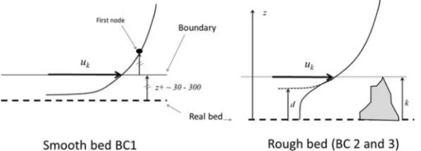
where 𝜅 is the von Karman constant, dw is the distance from the boundary and l0 the mix-ing length at the top of roughness. As the aim of the method is to integrate several kinds of boundary conditions, it is possible to describe them with the 3 conditions described here-after. They are based (except smooth boundary) on the description of a turbulent boundary layer. (1) 𝜌u𝜕u 𝜕x = − 𝜕p 𝜕x+ 𝜌gS0+ 𝜕 𝜕y ( 𝜌𝜈t𝜕u 𝜕y ) + 𝜕 𝜕z ( 𝜌𝜈t𝜕u 𝜕z ) (2) 0= −g𝜕h 𝜕x + gS0− 1 2 𝜕V2 𝜕x + 𝜕 𝜕y ( 𝜈t𝜕u 𝜕y ) + 𝜕 𝜕z ( 𝜈t𝜕u 𝜕z ) (3) 0= gS f+ 𝜕 𝜕y ( 𝜈t𝜕u 𝜕y ) + 𝜕 𝜕z ( 𝜈t𝜕u 𝜕z ) (4) 𝜈t= l2 m 𝜕u 𝜕l = l 2 m √ ( 𝜕u 𝜕y )2 + ( 𝜕u 𝜕z )2 (5) lm= 𝜅dw+ l0 (6) uk=u∗ 𝜅ln ( z− d z0 )
with u∗ the shear velocity, d the displacement height and z0 the hydraulic roughness. The value of d depends on the roughness arrangement and size. The value is chosen to be con-sistent with the study of Cassan et al. [3] (macro-roughness) and Nikora et al. [25] (vegeta-tion) which both propose a scaling length at the top of canopy l0≈ 0.15 k where k is the roughness height. The computation of the turbulent viscosity at the top of canopy leads to
l0= 𝜅(1 − d)k . Therefore the displacement height d is assumed to be equal to 0.63 k. 2.1.1 Smooth condition: BC1
When the flow is detected as being smooth at the boundary ( k+= ku
∗∕𝜈 < 20 ), the bound-ary velocity is computed with the Eq. 7, z = z + tmesh , l0= 0 (Fig. 1), where tmesh is the mesh size at the boundary.
When k+ ranges between 20 and 90, the functions from Ligrani and Moffat [19] are used. These functions allows reproducing as best as possible the wall friction whatever the flow regime smooth, transitional or rough.
2.1.2 From Nikuradse’s formula: BC2
Considering Eq. 6, the parameters d and z0 may vary with the arrangement of vegetation [21, 23] or macro-roughness [3, 29]. As they are responsible for the velocity profile near the bed, they must be predicted accurately. To be consistent with results on sand [26], we impose a hydraulic roughness height z0= 0.033 k. This value is the most commonly used for hydraulically rough bed and have been validated for a large range of flow. It is mostly pertinent when the water depth is high with respect to k. For example, this parametrization (in the integral form) is used in the modelling softwares HEC-RAS (1D) and Telemac (2D) in which the friction term can be defined as a function of the water depth.
2.1.3 From analytical resolution of the velocity within the roughness element: BC3 To take into account the flow within the roughness, the momentum equation could be solved considering drag force and turbulent terms [16]. Several studies used this method to compute the velocity distribution with vegetation or macro-roughness [1, 6, 13]. The (7) uk= u∗ (1 𝜅ln (t meshu∗ 𝜈 ) + 5.5 )
assumption of a logarithmic law above the roughness provides the values of d and z0 which are needed to compute the boundary condition uk at the top of canopy. Here, the approxi-mation for rough and dense roughness layer from Cassan et al. [3] is tested. But the meth-odology can be applied using other analytic formulations. For instance, Katul et al. [13] suggests to use the experimental correlation uk∕u∗= 3 for dense vegetation, where l0 is given by a canopy length scale. The law of Cassan et al. [3] for dense and gravel elements is incorporated with the following parameters Cd= 0.7 (drag coefficient), k∕D = 0.5 (D is the gravel diameter), C = 0.6 (density area). An approximation of the velocity at the top of canopy is given :
In Cassan et al. [3], the authors have shown that their model calibrated with the d84 of the bed granulometry should be similar to the friction law from Limerinos [20] which is vali-dated and relevant for river flow.
2.2 Computational method
The numerical procedure is developed with scripts already existing in the Matlab Tool-box dedicated to the resolution of partial differential equations (PDE) with finite elements method. All scripts are freely available on request.
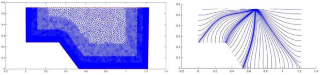
The cross section is meshed with triangular elements with a constant mesh size ( tmesh ). Afterward, the mesh is refined only near the bed (Fig. 2) to reduce the compu-tational time. For smooth flow, the minimum size should ensure that the distance between a first node and a boundary allows verifying the condition 30 ≤(z+ = u∗z∕𝜈) ≤ 100 where 𝜈 the molecular viscosity. For rough flow, the mesh can be larger and a maximum value of h / 30 is used. To start the PDE resolution an initial condition is given by considering a constant velocity deduced from the Manning equa-tion with n = 0.025 . In a first step, the equaequa-tion is solved with an uniform shear stress based on the hydraulic radius ( u∗0=√gSfRh ). The boundary condition at the free sur-face is a slip condition which leads to a maximum velocity at the free sursur-face. Although in practical case, the secondary currents involve a dip phenomenon, this pre-sent model does not solve this issue because the applications studied here are focused on boundary layer. For wall boundaries, the velocity uk is imposed considering the shear stress u∗0 . The Eq. 3 is numerically solved with the Partial Differential Equation Toolbox using a Finite Element Method. The velocity distribution is then used to (8) ( uk u∗ ) ≈ ( 4k l0 )1∕3 ( D(1 − 𝜎 C) kCdC )1∕3
Fig. 2 Mesh used for the experimental case (left). Ray normal to isovel corresponding to the geometry from Kean et al. [14] (right)
compute the normal lines (ray) to isovels. These lines start from the boundary, and are spaced with a constant length tmesh (or larger to reduce computation time) (Fig. 2). By applying the momentum balance to each sub-area A, it is possible to distribute the shear stress on the boundary lengths (P). Indeed the shear stress on the lateral ray is equal to 0 since the velocity gradient is null normal to this line. The value of u∗ is given by the momentum balance considering a constant friction slope ( u∗=
√
gSfA
P ). If the isovels are assumed to be horizontal, the method is equivalent to the Einstein method [8] which is the case for large river. In addition to providing vertical distribu-tion, the advantages of Kean et al. [14] method mainly appears for rivers during low-flow periods (complex cross section) and narrow channels (irrigation and waste net-works). Unlike the Einstein method, it is possible to consider the lateral boundary layer due to friction of vertical sidewalls. A second step consists in recomputing the velocity fields with a boundary condition uk deduced from the shear velocity u∗ obtained in the previous step. Several iterations with an adjusted relaxation constant are needed. The computation is stopped when a maximum number of iterations is reached (10) or if the residual criteria is smaller than 0.01. The computation lasts between 1 and 20 seconds depending on the section size and hydraulic conditions which impose the mesh size.
3 Experiments
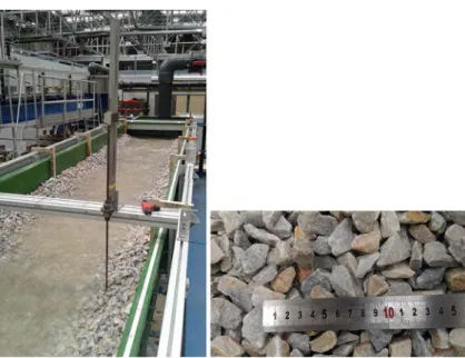
As already mentioned, the method is relevant for natural cross section in particular if the channel can be considered as narrow, if the transverse roughness is quite heteroge-neous or if specific frictions law are need. This kind of flow is typically encountered in mountainous rivers. Here, investigations are carried out with a scale model to focus on the influence of friction laws. Experiments were conducted in a tilting flume (1 m wide and 7 m long) at the Institute of Fluid Mechanics in Toulouse. A trapezoidal sec-tion was installed and covered with 2.5 cm pebbles (mean grain diameter) (Fig. 3). For slopes of 0.7, 1.2 and 1.7% and flow rates of 15.9, 22.6 and 41.2 l/s, the water depth at the centerline is measured with a point gauge at 4 m from the upstream end. In the result part it is checked that the application of the redistribution method should repro-duce the measured stage-discharge relationship and predict the evolution of the friction as a function of the water depth. Indeed, the Manning equation generates a Manning coefficient n varying from 40%: n varies from 0.03 to 0.044 (Table 1).
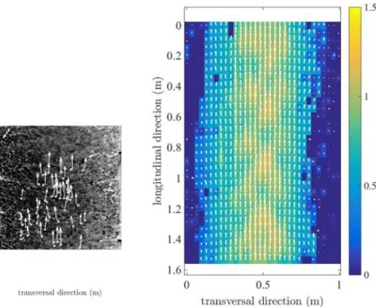
The experiments were completed with the surface velocity measurement for 5 addi-tional cases ( Q = 20 and 50 l / s and S = 0.5 , 1 and 2%). The method chosen is similar to Large Scale Particule Velocity Tracking (LSPTV) [32]. Floating balls with a 1 cm diameter were randomly distributed over the free surface and their trajectory were recorded with a fast camera (resolution 2K × 2K, 300 frames per second). More than 2000 images are captured for each experiment. The picture are thresholded considering their pixels intensity and the particules detected are deleted if their length is superior to 50% of the mean diameter (1 cm). The used algorithm is detailed in Ducrocq et al. [7], and the images were rectified with an homography matrix [28]. An example of the picture and the associated velocity vectors is given on Fig. 4. The final velocity field is recontructed by gathering all data in the same cell ( 64 × 64 pixels) (Fig. 4).
4 Validation of the numerical procedure
The validation of the numerical procedure is performed with 4 different type of experi-ments to explore several flow conditions where the procedure is pertinent compared to Einstein’s method or Computationnal Fluid Mechanics considered as time consuming. We focus on:
– Rectangular channel to validate the implementation of boundary condition.
– Experiments described in previous part to emphasize the interest to use an adequate friction law, in particular for low submergence flow.
– The experiments from Kean et al. [14] to illustrate a strong spatially distributed roughness and its implication on the velocity field.
Fig. 3 Experimental device and roughness
Table 1 Experimental results S Q h n
m/m (l/s) (m) 0.007 22.6 0.099 0.037 0.012 22.6 0.089 0.041 0.017 22.6 0.083 0.044 0.007 15.9 0.085 0.042 0.012 15.9 0.078 0.047 0.017 15.9 0.073 0.051 0.007 41.2 0.126 0.030 0.012 41.2 0.116 0.035 0.017 41.2 0.109 0.037
– The experiments from Wang et al. [34] with both a distributed roughness and a narrow open channel.
4.1 Rectangular channel
As the velocity field is concerned, the numerical procedure is firstly validated by consider-ing the simple case of a rectangular channel with a constant roughness. The objective is to ensure that the computation provides logarithmic profiles depending on the roughness height. The computations were performed for h∕B = 0.1 , 0.15, 0.2, 0.5, 1, 1.5, 2 with a constant width B = 1 m.
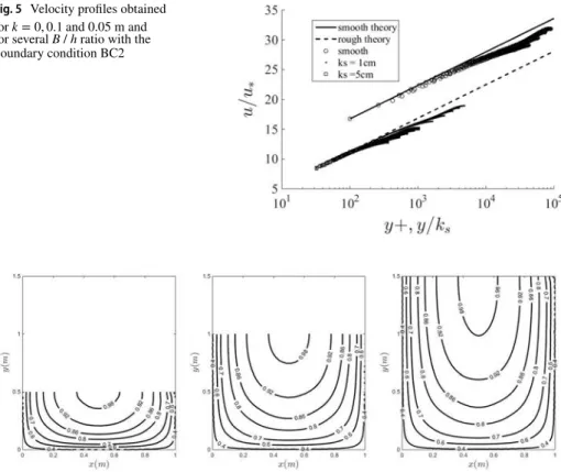
The Fig. 5 shows that for all runs, the velocity profile is consistent with the logarith-mic law near the bed. Mesh dependancy study has proved that the velocity profiles are not modified if tmesh<= l0 or z+< 300 for smooth cases. This boundary condition involves long computation time for a uniform mesh that is why a refinement is needed near the wall. In the upper region, the velocity is lower than the log-law profile unlike an empirical tur-bulent wall-bounded flow. The method is not able to reproduce a velocity higher than the logarithmic law because the slip condition imposes a zero-gradient at the free surface. For real flow, the higher velocity is due to both secondary currents and variation of the turbu-lent properties which are not taken into account in the computation. This systematic error is quite low as discharge and velocity near bed are concerned [2].
For the narrower channel flow, the simulated velocity at the surface tends to the loga-rithmic law. This behavior can be explained by the boundary layer at the sidewalls. Indeed their influence is sensitive at the centerline and then modifies the vertical profile in the upper part (Fig. 6).
Fig. 4 Recorded image and particule detected (left) and velocity field (m/s) for Q = 50 l/s and S = 1 % (right)
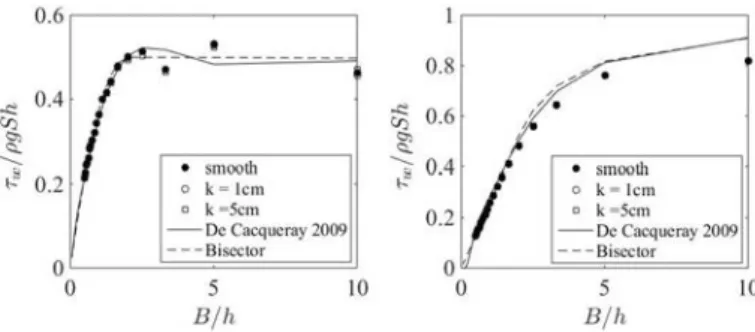
For rectangular channel, the repartition of the friction between bed and sidewall has been extensively studied. The most simple way to evaluate this distribution is to consider bisectors of the corners as lines normal to the isovel [15]. The bed shear stress distribu-tion is provided by the ratio of the wetted subarea (Sect. 2.2) delimited by the bed, the bisector and the free surface. For smooth channel Guo and Y. [10] elaborated an analytical solution to obtain the averaged shear stress on sidewall and bed of a rectangular channel. Cacqueray et al. [5] used CFD to improve the results by adding correction factors. These 2 approaches were validated with experiments from literature. The Fig. 7 confirms that the proposed method is also consistent with 3D model and thus with experiments which had validated the CFD results. The additional interest is that the method predicts a local description of the shear stress when the roughness height is not constant. As for veloc-ity field, some discrepancies with the experiments, due to secondary currents, could be expected [17].
4.2 Experiments at IMFT
The computed discharge is compared to our experimental values for the 2 kinds of bound-ary conditions (BC2 and BC3) on Fig. 8. BC2 and BC3 numerical procedures reproduce correctly the evolution of the stage-discharge relationship since the discharge is well calcu-lated for a given water depth and roughness height. The sensitivity to the roughness height
Fig. 5 Velocity profiles obtained for k = 0, 0.1 and 0.05 m and for several B / h ratio with the boundary condition BC2
is illustrated by varying this parameter. The first remark concerns the k value as function of the BC. With BC2, k is largely higher than the mean diameter of roughness even if only one value of k = 30 cm is used to compute the stage-discharge relationship for all slopes. The BC3 is more pertinent because k = 3 cm provides satisfactory estimate of the discharge (Fig. 8) and corresponds to the range of pebble diameters on the bed.
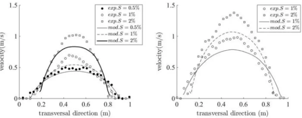
To validate the method with the present experiments, the surface velocity profiles obtained by LSPTV are compared to the velocity provided by the model (with BC3,
k= 3 cm) on the Fig. 9. The experimental velocity is obtained by averaging the velocity field in the longitudinal direction. For slope inferior to 1%, the model predicts the velocity surface with a small discrepancy for the entire profile. However the maximum velocity is underestimated at the centerline when slope increases. This gap could be related to second-ary currents or the fact that the wake law is not considered in the model. Moreover the experimental velocity field on Fig. 4 presents periodic variation which may be due to free surface interaction. Indeed, in the experiments, the Froude number becomes greater than 0.5 when the slope is superior to 1%.
4.3 Experiments from Kean et al. [14]
To emphasize the advantage of a better boundary formulation in a natural flow, the experiments from Kean et al. [14] are also taken into consideration. The lateral distribu-tion of roughness is the one given by Kean et al. [14]. In particular, the boulder diameter
Fig. 7 Bed shear stress distribution for rectangular channel (BC2) on sidewall (left) and on the bed (right) (Numerical results from [5])
Fig. 8 Comparison of computed and measured discharge as a function of the roughness parameter, for BC2 (left) and BC3 (right)
is 4.5 cm on the floodplain. The experimental data reveals the effect of the roughness height on the boundary layer and above large boulders (Fig. 10).
The computed velocity fields with BC2 and BC3 are in good agreement with those obtained by Kean et al. [14]. The same differences with experiments are observed and are attributed by Kean et al. [14] to secondary currents found experimentally in the bot-tom left corner. However the velocity is lower with BC2 and the total discharge is 367 l/s whereas the experimental one is 396 l/s. With BC3, the computed discharge is 400 l/s. It could be stated that the discharge is adequately described by the newly proposed method. But it must be noted that the side walls are smooth which explains the similar results for the 2 boundary conditions.
Fig. 9 Transverse profile of longitudinal velocity from experiments and proposed model for Q = 20 l/s (left) and Q = 50 l/s (right) at the free surface
Fig. 10 Velocity field: measured from Kean et al. [14] experiments (top) and computed with k = 4.5 cm with BC2 (left) and BC3 (right)
4.4 Experiments from Wang et al. [34]
We described a useful way to obtain quickly the velocity distribution for various cross sec-tion shapes and roughness heights. As a consequence, it could help to design structures where areas with low velocity are needed. This objective is essential for fish passage struc-tures as nature-like fishpass or artificial river. With the present method, the detection of low velocity area near the bank is improved, and the influence of the roughness height on this area can be determined in a design process. For small Australian fishes, Wang et al. [34] studied the advantage of adding roughness on culvert bed and sidewalls to enhance the passability of this structure. By reducing velocity near some walls, it appears possible to get a flow slower than the swimming abilities of small fishes. The method is a supplemen-tary tool to assess the modification of the structure conveyance as a function of the rough-ness. In a first step, the computed velocity is compared to the experiments in a scale model [34]. These experiments were conducted on a rectangular flume with a small roughness on the right sidewall ( k = 0.2 mm) and a larger roughness on the bed and on the left sidewall ( k = 20 mm). The bed slope is null and Sf is deduced from the water surface profile.
The Fig. 11 compares experimental velocity with simulated ones with the two kind of boundary conditions. The friction slope is deduced from the experimental Darcy-friction coefficient f = 0.07 [37]. It confirms that the method is pertinent since the predicted dis-charge is 0.0283 m3 /s for BC1+BC2 and Q = 0.0263 m3 /s for BC2 only ( Q = 0.0255 m3∕s in experiments). With BC1, the non symmetric field due to the smooth wall is visible even if it is overestimated. The k+ value is between 11 and 20 which is the limit for smooth wall. Then the difference could be due to the boundary condition and new calculations are performed with BC3 for all walls. This condition is better suited for prediction of the experiments (Table 2). Although a difference exists in the uppert part of the field between experiments and model, our results are consistent with the CFD simulation from Zhang and Chanson [37] computed with similar roughness height. This condition is therefore used for the following comparison (Figs. 12 and 13). It should be mentioned that the hydrau-lic roughness from Zhang and Chanson [37] has been kept to assess numerical methods. However it would have been possible to calibrate these values since law friction differs. Therefore, the discrepancy between numerical procedure and experiments would decrease significantly.
For the cases with the larger discharge , the method slightly overestimates the flow-rate ( Q ≈ 0.059 m3 /s against Q = 0.055 m3 /s in experiments cf. Table 2). The value f of the roughness description can explain it and k should be calibrated. This adjustment could be due to the roughness shape different from spherical elements corresponding to the BC2 condition.
Fig. 11 Experimental velocity fields from Wang et al. [34] for h = 0.12 m (left), simulation with a BC1 + BC2 (center) and only BC2 (right)
To evaluate the relevance of rough sidewalls, the percentage of wetted areas where the velocity is low is measured. It could be noticed that this percentage is almost constant for a given water depth whatever the discharge. The simulated area where U < Umean is in agreement with the experiments (Table 2). The simulation tends to underestimate the area for threshold velocity lower than Umean (i.e 0.25 Umean) but it could be due to the diffi-culty to measure and simulate this close wall region.
5 Implication for environmental applications
In comparison with a CFD calculation the present numerical procedure has several advan-tages. It could be easily adapted to complex cross section shape, the wall law can be easily modified and the number of parameters is reduced. But the main benefit is the computa-tional cost because only few seconds are needed for a river cross section. Therefore the
Fig. 12 Experimental velocity fields from Wang et al. [34] for h = 0.175 m and Q = 0.0556 l/s (left), h = 0.085m. and Q = 0.0261 l/s (center) and h = 0.155 m and Q = 0.0556 l/s (right)
Fig. 13 Computed velocity fields from Zhang and Chanson [37] for h = 0.175 m and Q = 0.0556 l/s (left), h = 0.085m. and Q = 0.0261 l/s (center) and h = 0.155 m and Q = 0.0556 l/s (right)
Table 2 Velocity distribution in a culvert cross section
Q ( m3/s) h (m) Umean m/s Umax m/s U < Umean (%)
Wang et al. [34] 0.261 0.129 0.423 0.755 45
Model (BC3) 0.256 0.129 0.42 0.71 47.8
Wang et al. [34] 0.0556 0.1743 0.667 0.957 45
procedure is particularly suitable for environmental applications where the knowledge of the velocity field is necessary. We provide here examples for which the procedure can bring quick solution for restoration, design or measurement issues.
5.1 Hydrodynamic of low submergence flow
The Fig. 14 presents the interest of the method to predict the area where the velocity may be low (see previous part about culvert passage). Indeed this bank zone is potentially rel-evant for fish spawning and ecological functions in a real river.
All 1D models can be post-treated with this method, then it could be used to evaluate the variation of velocity and sediment transport for long river. It may be a tool for diagnos-tic of aquadiagnos-tic habitat and river restoration for existing models. The knowledge of turbulent viscosity also helps to compute transversal or vertical transfer of suspended load or pollut-ant. Moreover the integration of Eq. 3 is consistent with the energy equation on which most 1D models are based. Incorporating this method in a 1D model could improve the preci-sion of the model by computing the head loss with various friction laws (e.g BC3). 5.2 Discharge from LSPTV measurements
Although the experimental and computed velocities do not totally agree for our experi-ments, the total discharge predicted by the model is similar to the experimental one. The maximal error is 10% (Table 3). As a consequence, the method can be coupled with LSPTV measurements to extrapolate the total velocity field. The ratio between the velocity
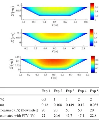
Fig. 14 Velocity distribution with the Cassan et al. [3] fric-tion law for Q = 15.8, 22.3 and 41.2 l/s (BC3 and k = 0.03 m)
Table 3 Discharge from numerical methods (BC3, k = 3cm) and PTV measurements
Exp 1 Exp 2 Exp 3 Exp 4 Exp 5
S (%) 0.5 1 1 2 2
h (m) 0.121 0.108 0.149 0.12 0.085
Q measured (l/s) (flowmeter) 20 20 50 50 20
surface and the averaged velocity can be known with more accuracy for each LSPTV measurements. Thanks to the low computation time, the procedure can also be used for statistical study which would give this velocity ratio as a function of cross section, water depth or roughness.
5.3 Design of real scale fish passage
For a design process of fish passages, the method allows obtaining results at a larger scale and with different roughness. Then the compromise between large low velocity area and sufficient hydraulic conveyance can be found. It is a complementary tool to design guide-lines proposed by Leng et al. [18].
The Fig. 15 represents the isovel obtained in a real culvert (2 m wide, Sf = 0.1 %) with a roughness of the left sidewall of 2 mm (concrete) and roughness of the bed and other sidewalls with k = 5 , 10 and 20 cm. These k roughness values are very large but it is an equivalent roughness size (related to the chosen friction law) that could be representative of specific macro-roughness.
The increase of the roughness clearly reduces the velocity and then the conveyance. The difference between the smallest and the largest roughness is not sufficient to exhibit a non symmetric velocity field except in the right bottom corner where velocity is reduced. Thanks to the method, it is possible to provide the stage-discharge relationship as a func-tion of roughness and waterdepth. As a consequence the method can be used for the design of other kinds of fish pass as artificial river or rock ramp.
5.4 Morphodynamic
The forces exerted on banks can have a non uniform lateral distribution which has an impact on the associated erosion. For the experiments of Kean et al. [14], the wall shear stress is better simulated where the roughness height ( k = 0.8 mm) is well defined i.e on the main channel bed (Fig. 16). It could be explained by the fact that k is in the range of Nikuradse law application. A discrepancy exists on the aluminum sidewalls which are smooth ( X < 0.35 and X > 1.6 ), then the transition formula of Ligrani and Moffat [19] may be responsible for the difference. Nevertheless the general trend is almost similar to the measured one. In particular the advantage to distribute the shear stress compared to an averaged value clearly appears. For the present experiments, the Fig. 17 exhibits the same variation from the averaged value. The lower shear stress on the banks can be used to study solid transport and forecast the evolution of bed during floods.
6 Conclusion
A method to compute the velocity distribution on a cross section has been presented. It is based on the consideration from Kean et al. [14] which predicts the longitudinal velocity with a mixing length turbulent model. The resolution is obtained with a Finite Element Method directly available in Matlab toolbox. Then the method can easily be used as a post processing of all 1D hydraulic models. The main improvement is the explicit description of the boundary condition, especially with the roughness height as a parameter which can be distributed laterally. For large river, the method tends to be similar to the Einstein method and then it is more pertinent for narrow channels. The validation has been performed by comparison with results from Kean et al. [14] and bed shear stress for rectangular and trap-ezoidal channels. It appears that phenomenon due to secondary currents as dip phenom-enon or wake zone are not reproduced by the method. However it is imperative to provide a good estimation of discharge as a function of roughness. Therefore it is justified to use it in design process of hydraulic structure where the flow is unidirectionnal such as fish passes. For large and narrow open channel flows, the method can be useful to integrate new friction formulae as those developed for macro-roughness or vegetation. Thanks to an ideal river example, the interest of an adapted formulation is demonstrated since the law of
Fig. 16 Bed shear stress dis-tribution for experiments from Kean et al. [14]
Fig. 17 Bed shear stress distribu-tion with the Cassan et al. [3] friction law (BC3) and k = 0.15 m, for Q = 2 , 8 and 16 m3/s
friction has been parametrized with observed roughness size instead of hydraulic rough-ness varying with hydraulic conditions. Lastly, the method could be useful to extrapolate LSPTV measurements and obtain a more accurate flowrate.
References
1. Cassan L, Laurens P (2016) Design of emergent and submerged rock-ramp fish passes. Knowl Manag Aquat Ecosyst 417(45):1–10. https ://doi.org/10.1051/kmae/20160 32
2. Cassan L, Belaud G, Baume Jean-Pierre, Dejean Cyril, Moulin Frederic (2015) Velocity profiles in a real vegetated channel. Environ Fluid Mech 15(05):1263–1279
3. Cassan L, Roux H, Garambois PA (2017) A semi-analytical model for the hydraulic resistance due to macro-roughnesses of varying shapes and densities. Water 9(9):637. https ://doi.org/10.3390/w9090 637
4. Chiu Chao Lin (1989) Velocity distribution in open channel flow. J Hydraul Eng 115(5):576–594 5. De Cacqueray Nicolas, Hargreaves David M, Morvan Hervé P (2009) A computational study of shear
stress in smooth rectangular channels. J Hydraul Res 47(1):50–57
6. Defina A, Bixio AC (2005) Mean flow and turbulence in vegetated open channel flow. Water Ressour Res 41:1–12
7. Ducrocq T, Cassan L, Chorda J, Roux H (2017) Flow and drag force around a free surface piercing cylinder for environmental applications. Environ Fluid Mech 17(4):629–645
8. Einstein HA, Banks RB (1950) Fluid resistance of composite roughness. Eos Trans Am Geophys Union 31(4):603–610
9. Ferguson R (2007) Flow resistance equations for gravel- and boulder-bed streams. Water Resour Res 43(5):W05427
10. Guo J, Julien PY (2005) Shear stress in smooth rectangular open-channel flows. J Hydraul Eng 131(1):30–37
11. Guo J (2017) Exact procedure for Einstein–Johnson sidewall correction in open channel flow. J Hydraul Eng 143(4):06016027
12. Huthoff F, Augustijn DCM, Hulscher SJMH (2007) Analytical solution of the depth-averaged flow velocity in case of submerged rigid cylindrical vegetation. Water Resour Res 43(6)
13. Katul G, Poggi D, Ridolfi L (2011) A flow resistance model for assessing the impact of vegetation on flood routing mechanics. Water Resour Res 47(8)
14. Kean JW, Kuhnle RA, Smith JD, Alonso CV, Langendoen EJ (2009) Test of a method to calculate near-bank velocity and boundary shear stress. J Hydraul Eng 135(7):588–601
15. Keulegan CH (1938) Laws of turbulent flow in open channels. J Res Natl Bureau Standards 21:707–740
16. Klopstra D, Barneveld HJ, van Noortwijk JM, van Velzen EH (1997) Analytical model for hydraulic resistance of submerged vegetation. In: Proceedings of the 27th IAHR congress, pp 775–780 17. Knight DW, Omran M, Tang X (2007) Modeling depth-averaged velocity and boundary shear in
trap-ezoidal channels with secondary flows. J Hydraul Eng 133(1):39–47
18. Leng X, Chanson H, Gordos M, Riches M (2019) Developing cost-effective design guidelines for fish-friendly box culverts, with a focus on small fish. Environ Manag 63(6):747–758
19. Ligrani Phillip M, Moffat Robert J (1986) Structure of transitionally rough and fully rough turbulent boundary layers. J Fluid Mech 162:69–98
20. Limerinos JT (1970) Determination of the manning coefficient from measured bed roughness in natu-ral channels. Geological Survey water-supply paper
21. Luhar M, Rominger J, Nepf H (2008) Interaction between flow, transport and vegetation spatial struc-ture. Environ Fluid Mech 8:423–439. https ://doi.org/10.1007/s1065 2-008-9080-9
22. Maghrebi Mahmoud F, Rahimpour Majid (2006) Streamwise velocity distribution in irregular shaped channels having composite bed roughness. Flow Meas Instrum 17(4):237–245
23. Nepf Heidi M (2012) Hydrodynamics of vegetated channels. J Hydraul Res 50(3):262–279
24. Nezu I, Nakagawa H (1993) Turbulence in open-channel flows. IAHR Monograph Series A. A, Balkema
25. Nikora N, Nikora V, ODonoghue T (2013) Velocity profiles in vegetated open-channel flows: com-bined effects of multiple mechanisms. J Hydraul Eng 139(10):1021–1032
26. Nikuradse J (1933) Laws of flow in rough pipes (stromungsgesetze in rauhen Rohren) VDI Forschun-gsheft 361. In translation, NACA Technical Memorandum 1292, 1950
27. Pagliara S, Chiavaccini P (2006) Flow resistance of rock chutes with protruding boulders. J Hydraul Eng 132(6):545–552
28. Patalano A, Garcia CM, Rodrigues A (2017) Rectification of image velocity results (RIVeR): a simple and user-friendly toolbox for large scale water surface particle image velocimetry (PIV) and particle tracking velocimetry (PTV). Comput Geosci 109:323–330
29. Raupach MR, Hughes DE, Cleugh HA (2006) Momentum absorption in rough-wall boundary lay-ers with sparse roughness elements in random and clustered distributions. Boundary Layer Meteorol 120(2):201–218
30. Rubol S, Ling B, Battiato I (2018) Universal scaling-law for flow resistance over canopies with com-plex morphology. Sci Rep 8(1):4430
31. Talbi Slim H, Soualmia A, Cassan L, Masbernat L (2016) Study of free surface flows in rectangular channel over rough beds. J Appl Fluid Mech 9(6):3023–3031
32. Tauro F, Piscopia R, Grimaldi S (2019) PTV-stream: a simplified particle tracking velocimetry frame-work for stream surface flow monitoring. Catena 172:378–386
33. Thornton C, Steven R, Morris Chad E, Fischenich JC (2000) Calculating shear stress at channel-over-bank interfaces in straight channels with vegetated floodplains. J Hydraul Eng 126(12):929–936 34. Wang H, Beckingham LK, Johnson CZ, Kiri UR, Chanson H (2016) Interactions between large
bound-ary roughness and high inflow turbulence in open channel: a physical study into turbulence properties to enhance upstream fish migration. Hydraulic Model Report No. CH103/16 School of Civil Engineer-ing, The University of Queensland, Brisbane, Australia. ISBN 978-1-74272-156-9
35. Wang H, Chanson H (2018) Modelling upstream fish passage in standard box culverts: interplay between turbulence, fish kinematics, and energetics. River Res Appl 34(3):244–252
36. Yang Shu-Qing, Tan Soon-Keat, Lim Siow-Yong (2004) Velocity distribution and dip-phenomenon in smooth uniform open channel flows. J Hydraul Eng 130(12):1179–1186
37. Zhang G, Chanson H (2018) Numerical investigations of box culvert hydrodynamics with smooth, unequally roughened and baffled barrels to enhance upstream fish passage. Tech rept. University of Queensland, School of Civil Engineering
![Fig. 11 Experimental velocity fields from Wang et al. [34] for h = 0.12 m (left), simulation with a BC1 + BC2 (center) and only BC2 (right)](https://thumb-eu.123doks.com/thumbv2/123doknet/14407601.511088/14.659.75.582.753.885/fig-experimental-velocity-fields-wang-simulation-center-right.webp)
![Fig. 13 Computed velocity fields from Zhang and Chanson [37] for h = 0.175 m and Q = 0.0556 l/s (left), h = 0.085 m](https://thumb-eu.123doks.com/thumbv2/123doknet/14407601.511088/15.659.76.586.84.241/fig-computed-velocity-fields-zhang-chanson-q-left.webp)
![[PDF] Labview avec Arduino capteur de temperature lm35 PDF | Cours Arduino](data:image/gif;base64,R0lGODlhAQABAIAAAP///wAAACH5BAEAAAAALAAAAAABAAEAAAICRAEAOw==)