Developments in the method of finite spheres : efficiency and coupling to the traditional finite element method

Developments in the Method of Finite Spheres: Efficiency

and Coupling to the Traditional Finite Element Method

by

Jung-Wuk Hong

B.S., Civil Engineering (1994)

Yonsei University

S.M., Civil Engineering (1996)

FEB 1

9

2004

LIBRARIES

Korea Advanced Institute of Science and Technology

Submitted to the Department of Civil and Environmental Engineering

in partial fulfillment of the requirements for the degree of

Doctor of Philosophy

at the

MASSACHUSETTS INSTITUTE OF TECHNOLOGY

February 2004

©

2004 Massachusetts Institute of Technology. All rights reserved.

r\

Author .... . .. I

Department of Civil and Environmental Engineering

September 15, 2003

Certified by . .

Certified by

Klaus-Jirgen Bathe

Professor of Mechanical Engineering

Thesis Supervisor

...

Franz-Josef Ulm

Apsociate Proffysor of Cigil and Environmental Engineering

Chairman, Thesis Committee

Accepted by

1wI

_{Heidi Nepf}

Chairman, Department Committee on Graduate Studies

Developments in the Method of Finite Spheres: Efficiency and

Coupling to the Traditional Finite Element Method

by

Jung-Wuk Hong

Submitted to the Department of Civil and Environmental Engineering on September 15, 2003, in partial fulfillment of the

requirements for the degree of

Doctor of Philosophy in Structures and Materials

Abstract

In this thesis we develop some advances in the method of finite spheres which is a truly meshless numerical technique for the solution of boundary value problems on geomet-rically complex domains. We present the development of a preprocessor for the auto-generation of finite spheres on two-dimensional computational domains. The techniques enable to determine the radii of the spheres as well as to detect the boundary of the analysis domain. The numerical integration for the calculation of stiffness matrices is expensive. However, by utilizing the compact support characteristic it is possible to transform the in-tegral equations into more efficient expressions. The improved equations reduce the effort of integration because for most terms, only line integrations are used. We also propose a new coupling scheme to couple finite element discretizations with finite spheres. The idea is that we can use finite elements and finite spheres simultaneously to utilize their mutual advantages. Hence, we can employ finite spheres only in areas where their use is efficient. In addition, we propose an enriching scheme which makes it possible to superpose spheres on conventional finite element topologies to reach a higher order of convergence in the numerical solution of problems.

Thesis Supervisor: Klaus-Jirgen Bathe Title: Professor of Mechanical Engineering

Acknowledgments

First, I truly appreciate the sincere guidance and encouragement of Professor Bathe. With-out his effort and passion, I would not have been able to pursue my studies at MIT. His inspiring suggestions and ideas have been always very helpful and essential whenever I met some difficulties in my research.

I would like to thank the members of my thesis committee, Professor Franz-Josef Ulm

and Professor Kevin Amaratunga for their sincere comments and encouragements through-out my studies. I am very glad to have the opportunity to discuss and interact with them. Also I would like to express my heartful thanks to Professor Jerome Connor and Professor Shi-Chang Wooh for their help.

I also wish to thank my lab members at the Finite Element Research Group, Dr. Uwe

Ruppel, Dr. Francisco Montins, Dr. Thomas Graetsch, Muhammed Baig, Bahareh Banija-mali, Philseung Lee, Jacques Olivier, and Omri Pedatzur for their help. Especially I would like to appreciate Dr. Suvranu De at RPI for his help and collaboration on the meshless techniques.

I am deeply grateful to my lovely family, my parents, my wife, Chihyun, my son,

Seung-Hyun, my sister, Sung-Hee, brother-in-law, Joon-Young and brother, Sang-Wuk, his wife, Jung-Min, and my lovely nephews and nieces. The cherishing encouragement from them was always the source of the energy for my study and life all the time.

I thank to all the Korean seniors and friends who helped and supported me. Their

List of Symbols

A Interior of a set A.

OA Boundary of a set A. a(., -Bilinear operator.

1 (-) Linear operator.

Open bounded domain, d = 1, 2,3.

F Boundary of Q.

n Outward normal vector.

B(xi, rj) {x E X: I|x - xH| < r} Open sphere of radius r.

S(xj, r1) {x E X

l

I|x

centered at x1.

W, Weighting function.

him(x) The mth shape function at node I.

h A global measure of the support radii.

f(k) kth derivative of

f.

x F y x is mapped onto y.

H7 Variational potential.

- L' or sum norm.

I1

||

I-

5

mn Kronecker delta. E Error requirement.

CN Unit cube in N-dimensional space. C() Continuous function on Q.

Ck(Q) k-times differentiable functions on Q.

Cok (Q) Functions in Ck vanishing on 9Q.

C(Q) Continuous function on Q.

Q(-)

M Space of model (approximation) functions.

Mp Space of polynomial model functions.

N Set of all natural numbers (positive integers).

PN Space of all polynomials in N variables.

Pd Space of all polynomials of maximum degree d. R Set of all real numbers.

Ktg, Ktn Stress concentration factors. k, Stress intensity factor. KZ Kolosov constant. G Shear modulus.

Contents

1 Introduction

1.1 O verview . . . . 1.2 Thesis outline . . . .

2 The Theory of the MFS Summarized

2.1 Approximation space . . . . 2.1.1 The Shepard function . . . . 2.1.2 Reproducing property . . . .

2.2 Galerkin weak form for N-dimensional spaces.

2.3 The Galerkin-based Method of Finite Spheres .

2.3.1 Approximation functions . . . .

2.3.2 Displacement-based formulation . . . .

2.4 Formulation for boundary conditions . . . .

33 . . . 34 . . . 36 . . . 37 . . . 37 . . . 40 . . . 40 . . . 4 5 . . . 50

3 Numerical Integration Theory

3.1 One dimensional numerical integration . . . .

3.1.1 Construction of quadrature rule by approximation . . . . 53 54 57 23 23 30

3.1.2 Approximation with polynomials

3.1.3 Orthogonal polynomials . . . . 3.1.4 Gauss formulas . . . .

3.1.5 Compound quadrature rule . . . .

3.2 Multi-dimensional numerical integration . . . .

3.2.1 Construction of formula by approximation.

3.2.2 Construction of formula by transformation

3.2.3 Generalized Cartesian Product Rules . . . .

3.2.4 Multivariate polynomial approximations . .

3.2.5 Polynomial Interpolation . . . . 3.2.6 Interpolatory formulas . . . . 61 . . . . . 62 66 68 . . . 69 . . . 71 73 74 76 . . . 77

4 Numerical Integration and Auto Sphere Generation for MFS 81

4.1 Improvement of analytical equations for numerical integration for inner sphere . . . . 82

4.2 Improvement of analytical equations for numerical integration for lens shape 89 4.3 Numerical integration for method of finite spheres . . . 91 4.3.1 Midpoint integration method for the inner sphere . . . 95 4.3.2 Integration on the lens domain . . . 95

4.4 New integration scheme for the inner spheres and boundary spheres . . . 98

4.5 Automatic generation of spheres in MFS . . . 102 4.6 A numerical result . . . 110

Introduction . . . . Coupling finite element discretizations with finite sphere discretizations

. . 111

. . 113

5.2.1 Construction of shape function on coupled domain . . . 116

5.2.2 Displacement-based method . . . 119

5.2.3 Formulation in the "pure" finite element domain QFE . . . . 119

5.2.4 Formulation in "pure" finite sphere domain QFS . . . . -. 121

5.2.5 Formulation in the coupled domain . . . 122

5.2.6 Assemblage of stiffness matrix and force vector . . . 127

5.3 Imposing the Dirichlet boundary condition . . . 128

5.3.1 When the restraint is applied in both normal and tangential directions 129 5.3.2 When the restraint is applied only in the normal direction or the tangential direction . . . 132

5.4 Enriching the finite element functions . . . 135

6 Examples of Coupling Methods 6.1 Tension and bending test of coupled elements. . . . . 6.1.1 Test geometry and loading conditions . . . . 6.1.2 Tension and bending test result of a simple plate 6.2 Specialized examples . . . . 6.2.1 Plate with a hole . . . . 6.2.2 Plate with a crack . . . . 139 . . . 139 . . . 139 . . . 142 . . . 142 . . . 145 . . . 154 163 7 Conclusions and Remarks

5.1 5.2

A Fundamentals of Functional Analysis

A. 1 Vector spaces . . . .

A.2 Hilbert space . . . .

A.3 Lebesgue spaces, LP(Q) . . . .

A.4 Sobolev spaces . . . . A.5 C'(Q) spaces . . . .

A.6 Dual spaces . . . .

167 . . . 167 . . . 168 . . . 170 . . . 171 . . . 171 . . . 173 B Cubature rules 175 B.1 Midpoint rule . . . 175

List of Figures

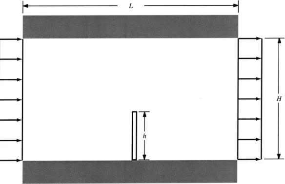
1-1 Isoparametric finite elements: (a) Due to small angle 6, this element be-comes "sliver" element. (b) There is an angle bigger that 180', so the one-to-one mapping is not satisfied. . . . 28 1-2 Fluid structure interaction 2-D model. In the channel, there is a slender

plate which interacts with the fluid flow. In the FEM modelling, this exam-ple may require extensive remeshing to simulate the behavior of the plate. . 28 2-1 A schematic of method of finite spheres . . . 35 2-2 A set of four subfigures . . . 41

2-2 Weighting function and derivatives (Cont'd): (c) Second derivative of WI.

(d) Third derivative of W1 . . . 42

2-3 A set of four subfigures . . . 44

2-4 Node distribution for the imposition of Dirichlet boundary condition. Nodes are arranged along the boundary to circumvent to have complicated inte-gration dom ain. . . . 51

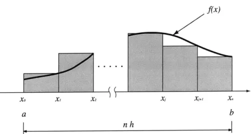
3-1 Riemann integration: right-side point rule is applied to integrate a function

f

3-2 Lagrangian polynomials. . . . 63

3-3 Legendre polynomials [1]. . . . 65 4-1 Pressure load is applied on cantilever plate. . . . 83 4-2 Finite sphere node arrangement. The nodes are uniformly distributed. . . . 83

4-3 Integrand distributions in Equation (4.1). . . . 84 4-4 Numerical integration scheme with newly derived equations from (4.20) to

(4 .23). . . . . 89 4-5 Figures of (a) inner sphere, (b) contact sphere, (c) boundary sphere on

Neu-mann boundary Ff, (d) boundary sphere on Dirichlet boundary I, . . . . . 92

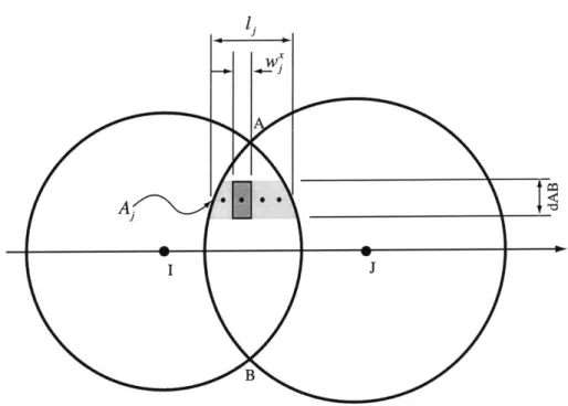
4-6 Inner sphere integration scheme. Midpoint rule is applied, and the sampling points are determined by Equations (4.36) and (4.37). . . . 93 4-7 Lens integration scheme, where A3 is the area of a strip, w7 is the width of

the sm all piece. . . . 94 4-8 A integration scheme for lens domain. Overlapped region is decomposed

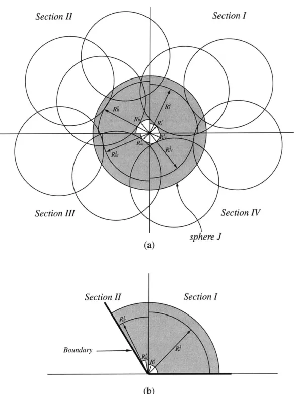
into pieces and the variables are calculated. . . . 94 4-9 New integration scheme for the inner sphere. (a) The sphere J is divided

into four domains based on the angle and determine neighboring spheres which are located in each region of angle. (b) Boundary sphere. ... 101 4-10 Automatic radius calculation scheme. . . . 102

4-11 Edge table generation scheme. Each row of the edge table contains in-formation about the nodes that are on an element edge. The format is (Ni,N2,flipping flag), where NI and N2 are the nodes connected be the edge and the flipping flag takes on a value of zero if the order is N2 < NI in the original connectivity and a value of 1 if the original order is reversed. 103 4-12 Inner sphere: The radius is determined by average value of node-distance

of neighboring nodes. . . . 104 4-13 Contact sphere: Node (I) has at least two neighborhood nodes which

re-quire special attention. The normal distance from node I to adjacent edges are computed and the minimum distance is adopted as radius . . . 105 4-14 Boundary sphere: The boundary nodes are obtained from the boundary

ta-ble. The radius of the sphere at a boundary node is selected as the minimum of the two nearest neighbor distances. The included angles 01 and 02 are used in the numerical integration . . . 106 4-15 Example of auto sphere generation: The plate has two holes and sphere

generation is implemented automatically. 175 spheres are distributed to cover the whole domain. . . . 107 4-16 Example of auto sphere generation: For the annular section sphere

genera-tion is implemented automatically. 37 spheres are distributed to cover the w hole dom ain . . . 108 4-17 Example of auto sphere generation: For the quarter of a plate which has

a hole sphere generation is implemented automatically. 168 spheres are distributed to cover the whole domain. . . . 109

4-18 Convergence comparison of finite element method and method of finite spheres. ... ... 110

5-1 Coupling finite element discretized domains with finite spheres discretized domains: (a) Coupling scheme and (b) computational domain decomposi-tion. We call QFE the domain which does not have any overlapping with finite spheres, QFE-FS the union of finite elements which have non-zero

overlap with spheres, and QFS the region which consists of spheres. . . . . 114 5-2 Enriching a finite element discretization with finite spheres: We call QFE

the domain which is not enriched with finite spheres, and QFE-FS, the

domain of finite elements enriched with spheres. It should be noted that there is no pure finite sphere domain. . . . 115

5-3 Shape functions hY E-FS ( hE-FS(X), PYE-FS(X) 4E-FS(x), hFiE-FS

and h E-FS(x) calculated by Equation (5.3) in a 1-dimensional case when

the spheres are located at the both ends, where R1, R2 1. . .. . -. . 117

5-4 Various kinds of Dirichlet boundary conditions: (a) u" and ut are fixed, (b) u1 is fixed and ul is free, and (c) ul is freed and ul is fixed. . . . 129 5-5 Stresses on the inclined surface. n is normal vector to the inclined surface

and t is tangential direction vector. . . . 134 5-6 Shape functions hYE-FS (x) h E-FS(X), E-FS(X) , 4 E-FS(X) hE-FSx),

and h FE-FS(x) in a 1-dimensional case when the spheres are located at the

6-1 Loading conditions for patch test of the coupling scheme. (a) unit tensile stress and (b) linear pressure distribution resulting in unit moment load are applied on the right end of the plate. For the material properties, E = 100

and v = 0.3. Element is under the plane strain condition . . . 140 6-2 Sphere arrangements on a 4-node element. (a) Two spheres are located on

the right side of 4-node element and (b) four spheres are placed on each node of4-node element. The coupled node means that it contains finite element node and finite sphere node simultaneously. . . . 140

6-3 Element refinements. (a) 1 element, (b) 2 elements, (c) 4 elements, (d) 8 elements, and (e) 16 elements are employed. L is the original length of the plate. W is the width of the plate with refinements. . . . 141 6-4 Convergence curves with different sphere allocations shown in Figure 6-2. . 144 6-5 Geometry of a plate with a hole in the middle of the plate. a is the radius

of the hole, b is the half of the width (L1) of the plate L2 is the length of

the plate and d = 2a is the diameter of the hole. The plate is subjected to lateral tensile pressure P under the plane stress condition. . . . 146

6-6 Stress concentration factors Ktg and Kt, for the tension of a finite-width

thin plate with a circular hole (Rowland 1929-30). . . . 148

6-7 ADINA result: 4096 9-node elements are used. Stress (o-,,) concentra-tion at the vicinity of the hole can be observed. The plate has the geome-try, boundary condition and loading condition in Figure 6-5. The Young's modulus is 100 and Poisson ratio is 0.3. in the plane strain condition. The maximum stress in horizontal direction is 3.008. . . . 149

6-8 Stress (o) concentration at the vicinity of the hole. The plate has the geometry, boundary condition and loading condition in Figure 6-5. The Young's modulus is 100 and Poisson ratio is 0.3 under the plane stress condition. 16 elements (4-nodes) are used. . . . 150

6-9 Stress (u-22) concentration at the vicinity of the hole. The plate has the

geometry, boundary condition and loading condition in Figure 6-5. The Young's modulus is 100 and Poisson ratio is 0.3 under the plane stress condition. 64 elements (4-nodes) are used. . . . 150

6-10 Stress (on2) concentration at the vicinity of the hole. The plate has the

geometry, boundary condition and loading condition in Figure 6-5. The Young's modulus is 100 and Poisson ratio is 0.3 under the plane stress condition. 256 elements (4-nodes) are used. . . . 151

6-11 Stress (-2) concentration at the vicinity of the hole. The plate has the geometry, boundary condition and loading condition in Figure 6-5. The Young's modulus is 100 and Poisson ratio is 0.3 under the plane stress condition. 16 elements (4-nodes) are used and the radius of each sphere added on the finite elements is 0.4. . . . 152

6-12 Stress (o) concentration at the vicinity of the hole. The Young's modulus is 100 and Poisson ratio is 0.3 under the plane stress condition. 64 ele-ments (4-nodes) are used and the radius of each sphere added on the finite elem ents is 0.2. . . . 152

6-13 Stress (o-r) concentration at the vicinity of the hole. The Young's modulus is 100 and Poisson ratio is 0.3 under the plane stress condition. 256 ele-ments (4-nodes) are used and the radius of each sphere added on the finite elem ents is 0.1. . . . 153 6-14 (a) geometry of a plate which has a sharp crack in the middle. The Young's

modulus is 100 and the poisson ratio is 0.3. The plate is under the plane strain condition. (b) local coordinate system . . . 155

6-15 Enriching scheme: Stress (o-2.) distribution along the vertical direction

from the crack tip. . . . 158

6-16 Stress (-2) concentration at the crack tip. The plate has the geometry, boundary condition and loading condition in Figure 6-14. The Young's modulus is 100 and Poisson ratio is 0.3 under the plane strain condition. 16 elements (4-nodes) are used. . . . 159

6-17 Stress (-x) concentration at the crack tip. The plate has the geometry, boundary condition and loading condition in Figure 6-14. The Young's modulus is 100 and Poisson ratio is 0.3 under the plane strain condition. 64 elements (4-nodes) are used. . . . 159

6-18 Stress (o-2) concentration at the crack tip. The plate has the geometry, boundary condition and loading condition in Figure 6-14. The Young's

modulus is 100 and Poisson ratio is 0.3 under the plane strain condition. 256 elements (4-nodes) are used. . . . 160

6-19 Enriching scheme: Stress (-2) concentration at the crack tip. The plate has the geometry, boundary condition and loading condition in Figure 6-14. The Young's modulus is 100 and Poisson ratio is 0.3 under the plane strain condition. 16 elements (4-nodes) are used and the radius of each sphere added on the finite elements is 0.5. . . . .

6-20 Enriching scheme: Stress (u-,) concentration at the crack tip. The plate

has the geometry, boundary condition and loading condition in Figure 6-14. The Young's modulus is 100 and Poisson ratio is 0.3 under the plane strain condition. 64 elements (4-nodes) are used and the radius of each sphere added on the finite elements is 0.25. . . . .

6-21 Enriching scheme: Stress (o-2) concentration at the crack tip. The plate has the geometry, boundary condition and loading condition in Figure 6-14. The Young's modulus is 100 and Poisson ratio is 0.3 under the plane strain condition. 256 elements (4-nodes) are used and the radius of each sphere added on the finite elements is 0.125. . . . . B-i

B-2

Midpoint rule integration. . . . . Gauss integration on a segment. . . . .

161

161

162

176

List of Tables

1.1 Various meshless methods which have been developed and the formulation principles are listed. MLS means that moving least square method. . . . 24

3.1 Quadrature abscissas and corresponding Gauss formula . . . 66 4.1 Establishment of subsections for sphere integration. . . . 99

6.1 Strain energy of coupled elements in tension and moment. Scheme (a) rep-resents two sphere allocation on the right side and scheme (b) means four sphere allocation on each node of 4-node element as shown in Figure 6-2. T means tension and M means moment. We consider the plane strain

con-dition, E = 100 and v = 0.3. The equivalent strain energy is calculated

by multiplying number of elements. The exact strain energy for tensional

loading is 0.00455 and for bending is 0.0546. . . . 143

6.2 Comparison of maximum stress value (o-72) in the plate with a hole shown in Figure 6-5. The exact value is assumed as 3.008. . . . 151

Chapter

1

Introduction

1.1

Overview

Frequently we need to analyze models subjected to continuous changes in the geometry such as large deformations in fluid structure interaction and crack propagation problem. To avoid large element distortions and collapse of elements and obtain accurate results, we need to remesh the model many times, and this calculation is cumbersome and expensive. Meshless techniques have advantages since sophisticated adaptive mesh generations are not needed.

Over the past eight years a variety of meshless techniques [2] have been developed such as the smoothed particle hydrodynamics method [3], the diffuse element method [4], the element free Galerkin (EFG) method [5], the reproducing kernel particle method [6], the partition of unity finite element method (PUFEM) [7], the hp-clouds method [8, 9], the finite point method, the local boundary integral equation method [10], the meshless local Petrov-Galerkin (MLPG) method [11], and the particle partition of unity method [12]. The

Method

Method of finite spheres [13] Diffuse element method [4] Element Free Galerkin Method [5]

Meshless local Petrov-Galerkin method [11] Finite point method [14]

Smoothed particle hydrodynamics [3] Reproducing kernel particle method [6] hp-clouds method [8,9]

Partition of unity FEM [7] Particle partition of unity [12]

System Equation Weak form Weak form Weak form Weak form Strong form Strong form Strong form Weak form Weak form Weak form Approximation Partition of unity MLS approximation MLS approximation MLS approximation Finite difference Integral representation Integral representation MLS approximation Partition of unity Partition of unity

Table 1.1: Various meshless methods which have been developed and the formulation prin-ciples are listed. MLS means that moving least square method.

names of meshless techniques and each basic principle used for the formulation are listed in Table 1.1.

On the other hand, we can also classify these techniques considering how to construct the shape functions into three major categories:

1. Finite integral representation methods:

(a) Smoothed particle hydrodynamic (SPH) method

(b) Reproducing kernel particle method (RKPM)

2. Finite series representation methods: (a) Partition of unity method (PU)

3. Finite differential representation methods:

(a) Finite difference method

(b) Finite point method

In the finite integral representation method, the unknown function is represented in a local domain via an integral form as

f (x) = f ()W(x - )d, (1.1)

where W( ) is a kernel or smoothing function. Finite series representation methods are well developed in FEM, and also applicable to meshless techniques. The function is defined as

f(x) = ao + aipi(x) + a2P2(x) + a3P3(x) + - - - (1.2)

where pi (x) are basis functions. Finite difference methods use Taylor series expansions to represent a function as

f (x) = f (Xo) + f'(xo)(x - a) + 1 f2(Xo)(x - a)2 +

---The weighting functions play an important roles in meshless techniques and many kinds of shape functions have been suggested,

1. Cubic spline function:

2/3 - 4s2 + 4s3 W(s) 4/3-4s+4s2 -4/3s 3 0 for s < , -2' for 1/2 s _ 1 for s > 1.

2. Quartic spline function:

1- 6s2 +8s 3 -3s4

W(s) =

0

for s < 1,

for s > 1. 3. Exponential weight function:

exp-(s/a)

2

0

for s 1,

for s > 1.

where a is a constant coefficient and we often use a =

distance from the node as

0.3. The variable s is the normalized

(1.7)

In the method of finite sphere we use the quartic spline function since it has a simple form of one single piece.

Although there have been some achievements in the formulations and theoretical proofs, the efficiency of meshless techniques is still a most important and difficult task. The method of finite spheres was developed by S. De. and K. J. Bathe [13]. In this technique, the do-(1.4)

(1.5)

(1.6)

ix - Xr l

the spheres is allowed. The only one requirement is that the union of spheres mush cover whole domain without any emptiness.

From the mathematical view point, the finite element method is a weighted residual scheme, and the solution is considered to reside in the considered vector space. Further-more, the error is orthogonal to a set of test functions. A great advantage of the finite element method is that Hilbert solution spaces are used via a weak formulation. In the finite element method, the domain is the subdivided into subregions, called "elements", and this is the most important concept in the finite element formulation since the governing equation is integrated over the elements in the weak form. However, to have a good quality of mesh, certain conditions should be satisfied.

In the isoparametric formulation, the Jacobian matrix is utilized to transform the coor-dinate system from local coorcoor-dinates of (x, y) to natural coorcoor-dinates of (r, s). The Jacobian matrix is non-singular when the one-to-one mapping condition is satisfied. It means that a point in the x-y plane should correspond to only one point in the r-s plane, and con-versely [2].

To be able to invert the Jacobian matrix, the element should not be distorted too much or folded. This restriction makes the mesh generation a enormous task in FEM analysis. Since this task requires more time than the actual numerical calculations in the analysis, avoiding the mesh generation is the main motivation of meshless techniques.

The creation of a mesh for the entire domain is the unavoidable prerequisite in solution based on finite element methods. Much time in the analysis is spent on mesh generation and checking the quality of the mesh. Especially, for large deformation problems, as for example shown in Figure 1-2, the quality of meshes affects the accuracy tremendously.

S 0 Angle is small Sr Line for r = -1/2 falls outside the element (a)

Figure 1-1: Isoparametric finite elements: (a) Due "sliver" element. (b) There is an angle bigger that satisfied.

L

to small angle 0, this element becomes

1800, so the one-to-one mapping is not

I1

HTh

I

H

Figure 1-2: Fluid structure interaction 2-D model. In the channel, there is a slender plate

S

r

Another restriction for the analysis is that the deformation cannot exceed the element size, Hence, adaptive procedures must be implemented at each time step of calculation in the FEM methods.

A variety of meshless techniques have been developed, but the currently available

tech-niques are still much more expensive than finite element methods. The main reason is that the shape functions are determined as non-polynomials although the functions are smooth

(E CI). Therefore, for the numerical integration more cost is needed than in the finite element method. Indeed, computational efficiency and reliablility are the most important issues for the development of the meshless techniques.

The method of finite spheres is a truly meshless technique, and the discretization is achieved by constructing Partition of Unity functions in the domain. The advantage of choosing the spherical local support is that the relative location can be described simply with their center coordinates and radii and the compact supportness ensures the narrow bandedness of the stiffness matrices.

In the traditional finite element method, the interpolation functions are polynomials which have the Kronecker delta property, and this ensures that the Dirichlet boundary con-ditions are satisfied in the weak sense. In addition, the basis functions make the numerical integration relatively convenient by the Gauss-Legendre quadrature rule. When the degree of the polynomial is known, the Gauss-Legendre rule can integration up to (2 x N - 1)

degree exactly. However, in the method of finite spheres the interpolation functions are not polynomials and they are rational functions. Hence more efficient numerical integration schemes should be developed to have required accuracy.

to generalize the numerical solution method, since we use conventional finite elements and finite spheres simultaneously. This provides several advantages because we can employ finite spheres only in those regions where they are effective. For example, in a crack propa-gation problem, we can add spheres easily to the tip of the crack to capture stress and strain concentrations. The finite element refinement around the crack tip can thus be largely dis-pensed with. In addition, the total cost of numerical integration is not that large since we use finite spheres on just certain local regions, not on the entire domain.

1.2 Thesis outline

A brief description of this thesis is as follows:

In Chapter 2, we summarize the basic formulations of the method of finite spheres based on the displacement approach. The construction of the approximation functions by the partition of unity is described.

In Chapter 3, the fundamental theory of numerical integration is summarized. We start from the one-dimensional problem and extend to multi-dimensional concepts. Basic princi-ples of Gauss formula, compound formula, orthogonal polynomials and the approximation theory are briefly described.

In Chapter 4, we derive the improved equations of the integrand functions by trans-forming the original equations into much simpler equations. This improvement reduces the dimension of numerical integrations in many terms. We address the automatic sphere gen-eration to cover the entire domain imported from a FEM package data file. The geometries

In Chapter 5, we present two new techniques to couple finite elements and finite spheres. The first scheme couples finite elements and finite spheres simultaneously and the second scheme is an enriching scheme. Different from existing schemes, the new techniques guar-antee the consistency in the coupled domain in the displacement field.

In Chapter 6, we give resuts regarding a simple tension and bending test with the cou-pling scheme and verify the convergence of strain energy. Then with the enriching scheme, a stress concentration phenomena are analyzed by solving a plate with a hole and a plate with a crack. The comparisons with analytical solutions are performed.

Chapter 2

The Theory of the MFS Summarized

The first step in the Galerkin procedure is to construct finite dimensional subspaces in a Sobolev space, where the unique solution is assumed to exist. The creation of shape functions is the most important part in the meshless technique, and the challenging issue is how to establish good shape functions with only nodes and radius. The requirements for the "good" shape functions are [15]:

1. Arbitrary nodal distribution.

2. The shape function should satisfy a certain order of completeness.

3. Compact support of the shape functions.

4. The algorithm should be computationally efficient.

5. The shape function should have the Kronecker delta property

It should be noted that the terms completeness and compatibility are used distinctively since the completeness/consistency means the capability of the field function approxima-tion method to reproduce the fields of lowest orders of complete polynomials at any point in the domain. The compatibility is the continuity of the approximation on the boundaries between the sub-domains.

In the method of finite spheres we choose partition of unity functions for construct-ing the trial function spaces. This choice allows the rigid body motion and zero strain condition. We discuss the partition of unity and the approximation properties of the trial function. The consistency, local approximation, continuity, and compact support are our desirable characteristic for the method of finite sphere. The consistency means polynomial reproducing property to ensure rigid body motion and constant strain states. This condition depends on the form of the partial differential equation. The compact support is that the function is non zero only on the concerned domain. This characteristic is essential to have a sparse matrix not fully coupled.

2.1 Approximation space

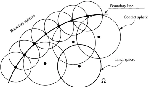
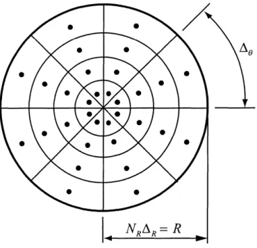
We adopted the partition of unity function to construct the approximation space and sphere domain for the compactness as shown in Figure 2-1.

The total analysis domain consists of the open compact domain Q and the closure I'. A set of spheres which have open domain B(x1, ri) and closure S(x1 , rj) covers the whole

Boundary sphere ru X2 xi XX3 x3 Ff

S

with the boundary (boundary sphere).

2.1.1

The Shepard function

We can start from the proposition [16] of

Proposition 2.1.1 Let G be an open set of R'. Let a family {U} of open subsets U of G

constitute an open base of G: any open subset of G is representable as the union of open sets belonging to the family U. Then there exists a countable system of open sets of the family U with the properties: the union of open sets of this system equals G, any compact

subsets of G meets only a finite number of open sets of this system.

Theorem 2.1.2 (The partition of unity) Let G be an open set of R'. Let a family of open

subsets

{G;

U)Gi.

iCI

{pj(x); j C J} of Cs (Rn) such that

for each

j

for every j C J, O < p (x) <1, (2.2)

E p (x) = 1forx c G. (2.3)

jCJ

The partition of unity function has these characteristics

N

1. Ep = i Vx E Q.

I=1

2.1.2

Reproducing property

Reproducing property is one of requirements for a good approximation space. The state-ment is that if any function Pk (x) is included in the local basis of each sphere, it is possible

to exactly reproduce it on the entire domain

(A).

Proof: We may write

N

Vh(X) Z1pI(X)pm(X) 'Im, (2.5)

I=mEa

and if we set alm = 6mk VI, where 5mk is the Kronecker delta, then this 6

mk is unity when

there exists the corresponding polynomial. Using the partition of unity,

N

Vh(X) = PI(X) Pm(X)aIm = Pk (2.6)

I=1 mEQ

2.2

Galerkin weak form for N-dimensional spaces

We consider open bounded domain Q c Rd(d - 1, 2, ... , n), and its close F. In the term

of partial differential operator,

Au =f in Q, (2.7)

in which linear differential operator A can be defined as

For the elasticity problem in n-dimensions, the operator [17] is

A = 1a (x) - + c (x), (2.9)

i,j=1 xix

and aij and c are bounded. We have Dirichlet and Neumann boundary conditions, and these are described in mathematical forms as

d

E ai(x)-n= f= on Ff (2.10)

i,j=1 ax

u = US onI7u (2.11)

where ni is the outward unit normal component along the boundary, F = F,

U

r.

fn

exact solution u and Uh orthogonal to the space of Vh (x) space. Therefore, we can establish

equations for each node as

(A(Uh) - f, hm) = 0, Vm E (2.12)

For generating approximation spaces with higher order consistency, the local approx-imation space Vjh = span{pm(x)} is defined at each node I, where pn is a polynomial

mEa

function and ' is an index set. The h is the superscript which represents the radius of the sphere.

the local basis polynomial functions, so we have

N

Vh=ZJVhP.

Vh = pjf.i

J=1

Therefore, any function Vh E Vh can be expressed as follows:

N

Vh Z 7hJn(x)aJjn

J=1 nE27

(2.13)

(2.14)

where hn (x) = pJ (X)pn (x), and we call hyn a shape function associated with nIh degree of freedom of node J. By Equation (2.14) and Green's theorem, we obtain the equation for the mth degree of freedom of Ith node as

KImjnajn fIm + fim, (2.15)

N E E I=1 MEG where KmJn = a(hm, hjn) n = c(x)himhJndQ _QI + _{j+ a} aij_(x _{0,x x} d9. (2.16)

It should be noted that a(., -) is bilinear operator, and

fIM = n fIm 1 j~ f (x)hmdQ, (2.17) (2.18) himniaij(x) Dx, drP fB(xj,rr) rI axj

where Q, = B(xj, r1)

l

Q.

2.3 The Galerkin-based Method of Finite Spheres

We briefly review in this section the basic formulation of the method of finite spheres.

2.3.1

Approximation functions

Based on the partition of unity requirement, we construct the basis functions. The domain

Q E Rd is an open bounded domain with I' its boundary as shown in Figure 2-1.

Each sphere consists of an open sphere BI(x1, RI) and its closure S1(RI), where x, is the center of the sphere and R, is its radius. The set of spheres must cover the entire

N

domain, i.e., Q c

U

the boundary; hence those spheres are considered to be boundary spheres.

fx - xf

We define a weighting function W(s), where s. = , which means that the

R,

weighting function is normalized by the radius of the sphere. This weighting function has compact support, and we have chosen a quartic spline weighting function of the following form as illustrated in Figure 2-2 (a).

W(s) = 1 - 6s1 2 +8s83 -3s 1 4; 0 < sI < 1. (2.19)

There are several well-known weighting functions for meshless techniques such as expo-nential, cubic spline, quartic, and SPH spline which all vanish at the boundary of support. Also, the first derivative vanishes at s, = 0 and s, = 1. The first derivative of the weighting

0.9 0.8 0.7 0.6 0.5 0.4 0.3 0.2 0.1 0 0.1 0.2 0.3 0.4 0.5 S (a) 0 -0.2 -0.4 -0.6 -0.8 -1 -1.2 -1.4 -1.6 1 08 0 0.1 0.2 0.3 0.4 0.5 S 0.6 0.7 0.8 0.9 1 0.6 0.7 0.8 0.9 (b)

Weighting function and derivatives: (a) Weighting

1.0 in one dimensional case. (b) First derivative of x = 0 and x = 1.

function W (x) when xi = W, with x. The derivatives

V V Figure 2-2: 0 and R = vanishes at I - . 1

2 0 -2 -4 -6 -8 -10 0 0.1 0.2 0.3 0.4 0.5 0.6 0.7 0.8 0.9 1 S (c) r -40 30 20 10 0 -10- -20- -30-0 0.1 0.2 0.3 0.4 0.5 0.6 0.7 0.8 0.9 1 S (d)

Figure 2-2: Weighting function Third derivative of W,

and derivatives (Cont'd): (c) Second derivative of W. (d)

Vl f

T?

-4

- I

function is

dW(si) _d 2 1283

1 =-12s1 + 24Lsj - 1s,

ds,

To calculate the first derivative of W1, we use the chain rule

OW _ OW₁ as1

Ox 81 Ox'

and we have

as (x - x₁) 1

Ox R1 2 si

finally, we have the simple form of the derivative as

aw

ax -12(1- s2) .

ax R 2

In the similar manner,

_W_ ( y- yI)

aw

ay

As an example, in two-dimensional the weighting function Wi(x),

a

- W₁(x)

PI (X) N,)

Ej=1 W

(x)'

I

For generating approximation spaces with higher order consistency, local approximation spaces VI = span{pm(x)} are defined at the nodes, where Pm is a polynomial function

mEQ (2.20) (2.21) (2.22) (2.23) (2.24) (2.25)

0.4 0.2 0 y x (a) 0.5 0.5 0 -0.5 _-0.5 -1 -1 (b) 0.5 0.5 0 --5 -0. -0. -1 -1 (c)

Figure 2-3: Weighting function and derivatives in two-dimensional domain: (a) Weighting function W (x), (b) , (c) .W(x)

and ! is an index set. Here h represents the radius of the sphere. We consider the case span {pm(x)} = {1, x, y} for two-dimensional problems.

m=0,1,2

The global approximation spaces Vh are generated by multiplying the partition of unity

function with the local basis polynomial functions,

N

Vh(x) = pIV

1=1

(2.26)

Therefore, any function Vh E Vh can be expressed as follows:

N

Vh hm(x)aIm,

I=1 mEQ

(2.27)

where him(x) = PI(x)Pm(x), and we call him(x) the shape function associated with the

mth degree of freedom of node I, and aim its coefficient.

2.3.2 Displacement-based formulation

We consider the following variational form [2].

I- ET (u)r(u)dQ

2

J

1

2

If

The term R is for the externally applied body forces, surface traction and prescribed dis-placements, 91= ju'fB dQ+ f UT fsd + fuT(U _ u)d, (2.28) (2.29)

where strain vector cT =

[eC2

displacement field, fP is the prescribed surface traction vector on the boundary Ff, u is the

prescribed displacement vector on the boundary F, and fB is the body force vector. The strain-displacement relation is e = Ou _{in Q,} where

a-

=

a/ax

a/ay

By the linear elastic constitutive law,

r = Ce(u) in Q (2.32)

In Equation (2.29) fP is the traction vector on the Dirichlet boundary, and fP is the

pre-scribed traction vector on the Neumann boundary rf,

u = [us(x, y) vs(x, y)], fu = NCE(u) on IF, VsT = [N r]T = [fx(x, y) fy"(x, y)] on

P

The matrix N has the direction cosine components of a unit normal outward vector as

n[ 0 ny

N =,

0 ny nx

and the elasticity matrix is

C11 C1 2 0

C12 C11 0

0 0 C33,

where for the plane stress condition the components of elasticity matrix are

E

C11 - V2

Ev

c = 12 ' c_{3 3} =

and for plane strain conditions,

E(1 - v)

(1 + v)(1 - 2v)'

Ev

C₁₂ = (1I+ v)(1 _{- 2v)'}

where E and v are the Young's modulus and Poisson's ratio of the elastic material respec-tively.

By invoking the stationary of H in Equation (2.28) we obtain

ET(v)CE(u)dQ vTfBdQ +

1r

f

fr"

_+v)'

4

S=4

where H1(Q) is the first order Hilbert space. The approximation for the displacement field can be written as where U = [aio N u(x, y) ZZ Hjn(x, y)ain J=1 nEd

an1 CE1 ... ]T and aj,, = [U-'"

= H(x, y)U, (2.41)

v "]. The displacement

interpola-tion matrix and strain-displacement matrix are respectively:

Hj(x, y) = hn (x, y) 0 , Bj.(x, y) = 0 1 han (X, Y) h., (x, y) 0 0 hin~ (x, y) hJn,(x, _y) han, (x, y)

where ha,(x) = pJ(X)pn and derivatives in x- and y- coordinates are

hJn,(x) = pJ,(X)Pn + pJ (x)pn,,

hJn,,(x) = PJ,y (X)Pn + PJ (X)Pn,y.

Finally, the discretized equation for node I, degree of freedom m, is

N

S

E

J=1 nEG

(2.42)

(2.43) (2.44)

where

KImJn = B TCBjndQ,

fnIM _(2.46)

fim = Him fBdQ (2.47)

and fim imposes the displacement/force boundary conditions [18]; for example, for a sphere intersecting Ff, we use

f1m f fB1 Hmfsd]P. (2.48)

In equations (2.46) and (2.47), Q, is the intersection of Q and BI(x, RI). On the other hand, if the sphere corresponding to node I has nonzero intersection on the Dirichlet bound-ary, then we have

(2.49)

N

fim = KUImJna Jn - fUIm, J=1 nEQi

where

HimNCBJnd + _{BImCNT H} Jd

fnB1

fRUm = Jr.flB1 BIm CNTu'dF.

It should be noted that the matrix KU is symmetric.

KUjmJn =

and

fF, fnB1

(2.50)

2.4 Formulation for boundary conditions

In meshless techniques, the imposition of the Dirichlet boundary condition and Neumann boundary condition incurs more complicated schemes than in the finite element method. However, still it is possible to handle this problems efficiently with a simplified scheme. In this section we discuss how to impose the boundary conditions derived in Equation (2.10) and (2.11) in the method of finite spheres considering the efficiency.

In the finite element method, because of the Kronecker delta property of the shape func-tions, only the nodes which correspond to the Neumann boundary condition are considered for the calculation of the consistent load, but in the method of finite sphere the shape func-tions do not have the Kronecker delta property, so we need to consider all the nodes which have non-zero intersection with the Neumann boundary. For example, let B1 n

f

intersection of the sphere I and the boundary Ff, then the union of B, f1 and B,

n

f

fm

Similarly, for the Dirichlet boundary condition in the finite element method only the nodes located on the Dirichlet boundary are considered to impose the Dirichlet boundary condition. Hence homogeneous boundary conditions can be exactly simulated.

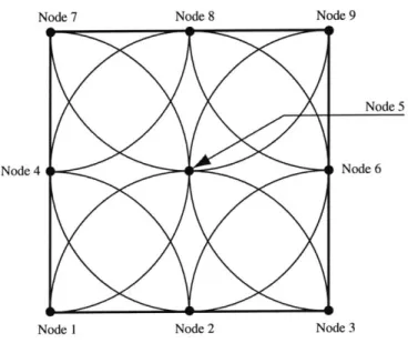
In the method of finite spheres, the shape functions do not have the Kronecker delta characteristic, so we introduce a technique to handle the Dirichlet boundary condition as in the finite element method [13]. The nodes on the boundary are distributed to have the same

Boundary lie

Contact sphere

Inner sphere

Figure 2-4: Node distribution for the imposition of Dirichlet boundary condition. Nodes are arranged along the boundary to circumvent to have complicated integration domain.

radii, and the inner spheres near the boundary do not have non-zero intersections with the boundary as shown in the Figure 3-1.

This ensures that the shape functions along the boundary have the Kronecker delta characteristic. Recalling the definition of p1(x) in Equation (2.25),

W1 (x) pi(x)

--ZE

1

_t

_Wy(x)

W1(x)

W(x)

To implement this technique, for the homogeneous boundary condition, we can elim-inate the rows and columns corresponding to the nodes which have non-zero intersection with the Dirichlet boundary.

Chapter 3

Numerical Integration Theory

The calculation of integrals is an essential task in the finite element method. Also, in mesh-less techniques, this task is most important. Tremendous amount of textbooks and articles are available [19-23]. However, the new concept of method of finite spheres demands some innovative ideas specific for our scheme. The term quadrature is frequently used for one-dimensional integration and term cubature is common for multi-dimensional integra-tions. This chapter gives a comprehensive and concise summary of numerical integrations including some fundamental theorems.

In the one-, two-dimensional cases, the required matrix integrations in the finite element and finite sphere calculations have been written as [2]

Jf

I

iji

f (x, y) are integrand functions in the matrices, and R, are error remainders which are not

f f(x)dx = cif (xi) (3.3)

J

f

y)dxdy

=

cjf (xi,

yi)

(3.4)

i~j

3.1 One dimensional numerical integration

Numerical methods for discretizing and approximating integrals are based on the use of appropriate integration formulas [24]. For the one dimensional integration problem, we have the integration rule

n

Q(f) Qn(f) ~~ cif (Xi), (3.5)

where ci is the integration weight,

Q

f

f

In many cases, quadrature formulas have symmetries as

when the abscissas xi, .. . , x,, of all practical quadrature formulas

Q,

integra-tion is

R.(f) ~~ f(x)dx ~ E(i+1 - xi)f((), (3.7)

where R(-) is the Riemann sum operator, E [xi, xi+1] for i = 1, 2,. . . , n. It is possible to

approximate any Riemann integrable function with any arbitrary accuracy requirement E. The simplest way to obtain a converging sequence of the Riemann integration is to divide the interval [a, b] into n subdivisions of equal length as:

xi = a + ih, i = 0, 1, ... , n; h= a .b (3.8)

n

The choice for j can be either left-side end point or right-side end point of the subdivi-sions. We use notations R2ft for left-side end point rule and R'ight for right-side end point rule. When we set the exact analytical integration value of the function

f

dis-cretization error {Rn(f) - I(f)} can be estimated in terms of modulus of the continuity. Theorem 3.1.1 Iff G C[a, b] and the integration domain is divided into n equal segments

having (n + 1) abscissas from x0 to Xn, then

fR right(f) - I(f) < (b - a) x f; b (3.9)

f(x) Xo a

Figure 3-1: Riemann integration: right-side point rule is applied to integrate a function

f(x) from a to b.

Proof When we apply right-side end point rule of Riemann integration for a given

func-tion

f

n b

|Rright (f) - = h f(x jb f

i=1

Since hf(xi) =

f,

h( f(xi) i=1 fb _{f(x)dx = (} n xi [f(xi) -ai1 i i_ f (x)]dx n xi <zfx t -n xi =1 xi_1

If(xi)

where

X(f; 6) = sup{ff(x1) -

f(x

3.1.1

Construction of quadrature rule by approximation

More effective quadrature rules can be obtained by approximating the function

f

model function g

E

approximation value 1(g) as the integration value for the exact integration of 1(f). This assumption is valid only when the model function can be described as a simple function, so the polynomial functions are most promising model functions. If the model function g satisfies

I 9 - f|| 1" 5 b(3.11)

where E is error requirement, then the error bound becomes

|I(g) - I |=

Jb

ab b

< f g(x) - f(x)ldx

j

)(3.12)

Hence, the approximation function which is close enough to the function

f

In many practical integration, it is quite often required to integrate some functions which are the product of w(x) and f(x), where w(x) is a weighting function which is known in analytical forms. Now we denote this kind of integration as product integration, and the notation is

I.(g) = I(wg). (3.13)

By this scheme, the resulting rule is called product rule. This integration is valid only when

the weighting functions can be expressed analytically, regardless of the space of model functions. The condition estimate for the validity of product integration can be derived as:

Iw(g) - = fw(x)g(x)dx -W(A - Jw(x)f(x)dx

<

J

|

Iw||W|g

O-f||

where I|- IL, is L1 norm. When the weighting function is absolutely integrable in the range of [a, b], then the error is proportional to the I1g(x) - f(x)|I L. Product rule is good for