Coupling between a Particle In Cell method and a H 1-conform mixed spectral finite element approximation of Maxwell's equations

(1)

HAL Id: hal-01956673

https://hal.archives-ouvertes.fr/hal-01956673

Submitted on 17 Dec 2018

HAL is a multi-disciplinary open access archive for the deposit and dissemination of sci-entific research documents, whether they are pub-lished or not. The documents may come from teaching and research institutions in France or

L’archive ouverte pluridisciplinaire HAL, est destinée au dépôt et à la diffusion de documents scientifiques de niveau recherche, publiés ou non, émanant des établissements d’enseignement et de recherche français ou étrangers, des laboratoires

Coupling between a Particle In Cell method and a H

1-conform mixed spectral finite element approximation

of Maxwell’s equations

Gary Cohen, Alexandre Sinding

To cite this version:

Gary Cohen, Alexandre Sinding. Coupling between a Particle In Cell method and a H 1-conform mixed spectral finite element approximation of Maxwell’s equations. The 10th International Conference on Mathematical and Numerical Aspects of Waves, Jul 2011, Vancouver, Canada. �hal-01956673�

(2)

Coupling between a Particle In Cell method and aH1-conform mixed spectral finite element approximation of Maxwell’s equations

G. Cohen†,∗, A. Sinding†,∗∗

†_{INRIA Rocquencourt, Le Chesnay, FRANCE.} ∗_{Email: gary.cohen@inria.fr}

∗∗_{Email: alexandre.sinding@inria.fr}

This paper describes the coupling between a Particle In Cell (PIC) method and a H1_-conform

mixed spectral finite element approximation of Maxwell’s equations for the approximation of low dense plasmas. It uses the H1_{-conform mixed}

spectral method already described in [2]. As parti-cle methods themselves are a classical subject, we mainly focus on the coupling between a finite el-ement method on an unstructured grid and a PIC method. This subject has already been studied for a coupling between a PIC method and a discontin-uous Galerkin scheme [4], but its still a challenging subject and the rehabilitation of continuous meth-ods to this aim hasn’t been studied yet. The critical point lies in the coupling between an Eulerian ap-proximation of the fields on an unstructured grid and a Lagrangian description of particles motion. This point can heavily penalize the global cost of the algorithm, if not taken into account carefully. In the next sections, a few techniques are intro-duced and compared to each other in order to ob-tain an efficient coupling algorithm between these two methods.

Introduction

Particle methods for the approximation of Vlasov equations mimic the miscroscopic and nat-ural model of plasmas. In such a model, all charges are taken into account individually and interact with each other. As the number of particles at stake is far too big for the current computational capacities, one has to consider an alternative de-scription with less particles. This is done by con-sidering macro-particles, whose charge approxi-mate the charge density given by Vlasov’s equa-tion. Macro-particles motion is described in a La-grangian frame by:

               xk dt = vk, pk dt = q(E(xk, t) + µ(xk)(vk×H(xk, t))), xk(0) = x 0 k, vk(0) = v 0 k, (1) fork ≤ N , in which N is the number of particles.

Equation 1 is approximate in time by a leap-frog scheme, which is only of order 2, but much easier to take into account than a Runge-Kutta scheme.

Maxwell equations are given by:

(

ε∂tE − ∇ × H= −J,

µ∂tH+ ∇ × E = 0,

(2) and approximate by aH1_{-conform mixed spectral}

finite element method such as described in [2]. In order to couple this two methods, one must be able to determine the current induced by parti-cles motion on each grid point, and conversely to determine the fields applied on each particle.

Interpolation considerations

When coupling particle methods with finite ele-ment methods, there is an obvious way to interpo-late the fields on each particle. For a particlek, we

have:

Ek=

X

i

Eiϕi(xk), (3)

withϕi the Lagrangian interpolation functions on

quadrangles in 2D (or hexaedra in 3D), and Ek

the electric field value at the particle position. For the inverse interpolation, on the other hand, the Dirac function is not sufficiently smooth to have an accurate approximation of the current (or

(3)

the charge density) on the grid points. For exam-ple, if a particle is not located on a grid point, its influence won’t be seen by the fields. To this aim, shape functions are introduced, which are compact and smooth distributions that approximately span the area of a cell. Traditionnally, and for a coupling with finite difference methods, splines of various orders are used, but not well suited for a coupling with high order methods on unstructured grids. In the following, we consider the choice proposed by Jacobs and Hesthaven in [4]:

S(r) = α + 1 πR2 (1 − ( r R) 2 )α. (4) withR the influence radius, and α the order of

ap-proximation.

In order to obtain a stability condition (see pages 152 to 154 in [5]), our interpolation strategy differs from the one described in [4]. We use the shape functionS, for both interpolations, and for a

parti-clek, Ekand Hkare then given by

       Ek= Z Ω E(x)Sk(x)dx, Hk= Z Ω H(x)Sk(x)dx. (5)

The inverse interpolation is done in a classical way as descibed in [4].

In order to reduce the cost of this interpola-tion steps, we must determine which grid points have an effective interaction with a particle located within a given cell of the Eulerian grid.

Particles’ tracking Tracking strategy

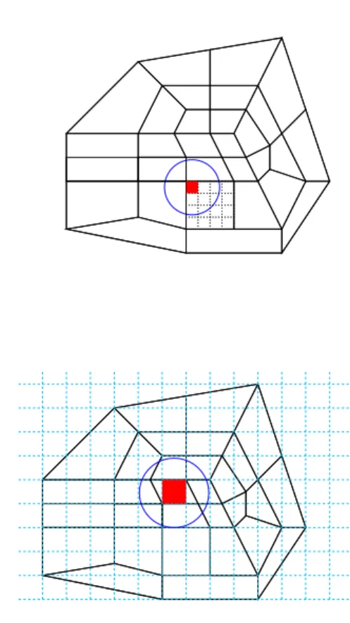
To determine in wich cell of the Eulerian grid a particle lies, one can consider various strategies. The most obvious one, is a localisation directly on the Eulerian grid. But to reduce the interpolation costs, we choose to compare two approaches (see figure 1):

• tracking domain 1: a subdivision of the

Eule-rian grid

• tracking domain 2: a cartesian box containing

the computational domainΩ

Figure 1: Influence zone of a cell.Top figure: tracking domain 1, bottom figure: cartesian box

containing the computational domainΩ.

In both cases, the subdivsion step is chosen so that the cell have a size of approximatelyR/3.

These two methods give approximately the same results in terms of interpolation costs (see pages 131 to 133 in [5]), the differences between them appear in the following paragraph.

Tracking algorithm

A first choice, is to map the particles coordi-nates onto the unit reference element for each cell of the Eulerian grid. The problem is that, for un-structured grids, this mapping is bilinear in2D and

threelinear in3D, making this step very expensive.

However for the tracking domain 2, the mapping function is linear, making it an interesting alterna-tive.

(4)

algorithms such as described in [3], in which no inversion of the mapping function is needed. In this algorithm, we dynamically follow the particle from cell to cell between two time-stepst and t + 1

(see figure 2). The algorithm only relies on con-nectivity properties of the mesh (common face be-tween two elements, normal to a face), which are stored when reading it.

Pt Pt+1 c1 c2 c3 ◦ ◦ t n1 n2 n3 n4 P ◦◦ c1 I1

Figure 2: Dynamic tracking of a particle.

Remark 1 Concerning the tracking of particles on a subdvision of the Eulerian grid, an interest-ing alternative is a two-stage algorithm. In the first step, the particle is located on the Eulerian grid, and in the second step, the particle is located on a subdivision of the given cell. This way, the localisation cost is globally divided byN r, where N is the number of particles, and r the order of

approximation. Boundary conditions

Boundary conditions for particles can be divided into two components as suggested in [4]. The first one concerns boundary conditions for the particles,

the second one is a boundary condition for the vir-tual cloud of radiusR associated with the particle.

Particles boundary conditions

Boundary conditions for particles can be of three types:

• elastic (fully or partially) boundary condition, • absorbing boundary condition,

• transparent boundary condition.

One major advantage of the dynamic tracking technique is that all boundary conditions for the particles are immediately taken into account. As we follow the particle from cell to cell by deter-mining which face of the cell has been crossed, each time this face is a boundary face, we only have to apply the associated condition for the par-ticle. We already know the normal to this face and no further operation is needed.

Cloud boundary condition

Cloud boundary conditions are designed so that a particle is not abruptly eliminated or introduced in the domain. An example for a metallic bound-ary condition is given in [4]: whenever the area of the shape function crosses the boundary, a virtual anti-particle of charge (-q) is placed on the other side of the boundary, so that the associated charge goes smoothly to zero as the particle encounters the metallic wall.

Unfortunately, in order to apply such a method one has to know the distance between the particle and the boundary everywhere in the computational domain. An interesting solution which has been tested is suggested in [4]. It consists in solving a Level Set equation in a preliminary step, so that the distance from the boundary is known on every grid point (see [5] for numerical illustrations).

Another alternative is given by using the track-ing domain 3. In this case, the tracktrack-ing domain is a cartesian grid in which the computational domain is included. By choosing a box slightly larger than the domain at every boundary point, one can intro-duce or eliminate particles smoothly. We only need

(5)

to wait until the cloud influence area has no inter-section with the boundary to eliminate the particle. In the same way particles created on a boundary, are introduced outside the domain.

Numerical results

After many tests, we choose dynamic tracking of the particles on a cartesian grid slightly larger than the computational domain in order to have an efficient coupling algorithm. This way boundary conditions for the particle are immediate and we don’t have to solve a LevelSet equation which can be long and expensive on very distorded meshes (oscillations near the steady-state even with a dif-fusion term). The charge conservation is forced whenever it is necessary, using a Boris correc-tion [1]. Numerical results for an electron beam and for Landau damping in2D can be found in [5].

Charge conservation for high order methods

In order to show the interest of high order meth-ods for a coupling with an particle in cell method, figure 3 gives theL2_{error on the divergence of the}

electric field for the electron beam simulation.

0 1 2 3 4 5 6 7 8 x 10−9 −3 −2.5 −2 −1.5 −1 −0.5 0 0 1 2 3 4 5 6 7 8 x 10−9 −3 −2.5 −2 −1.5 −1 −0.5 0 0.5 1 1.5 t log 10 (||div( ε E)− ρ ||/|| ρ ||)

Figure 3: semi-logL2_{error on the divergence of}

the fields for aQ5approximation. Top figure:

J = 1, bottom figure: J = 3000.

We can see that in both cases, this error remains lower than1%, without any correction of the fields.

For a strong coupling case (second figure in 3) however, the error tends to grow during the sim-ulation, suggesting that for long time simulations a periodic correction of the fields would be neces-sary.

References

[1] J. P. Boris. Relativistic plasma simulation— optimization of a hybrid code. Proc. 4th Conf.

on Num. Sim. of Plasmas, pages pp. 3–67,

November 1970.

[2] G. Cohen and A. Sinding. Non spurious mixed spectral element methods for maxwell’s equa-tions. To be submitted.

[3] A. Haselbacher, F. M. Najjar, and J. P. Ferry. An efficient and robust particle-localization al-gorithm for unstructured grids. J. Comput. Phys., 225(2):2198–2213, 2007.

[4] G. B. Jacobs and J. S. Hesthaven. High-order nodal discontinuous Galerkin particle-in-cell method on unstructured grids. J. Comput. Phys., 214(1):96–121, 2006.

[5] A. Sinding. Approximation du système de Vlasov-Maxwell : étude de solveurs Maxwell pour un couplage avec une méthode particu-laire. PhD thesis, Université Paris Dauphine,