HAL Id: hal-01103105
https://hal.sorbonne-universite.fr/hal-01103105
Submitted on 14 Jan 2015
HAL is a multi-disciplinary open access archive for the deposit and dissemination of sci-entific research documents, whether they are pub-lished or not. The documents may come from teaching and research institutions in France or
L’archive ouverte pluridisciplinaire HAL, est destinée au dépôt et à la diffusion de documents scientifiques de niveau recherche, publiés ou non, émanant des établissements d’enseignement et de recherche français ou étrangers, des laboratoires
Vitale, Fayçal Rejiba, Nicolas Flipo, Roger Guérin
To cite this version:
Sylvain Pasquet, Ludovic Bodet, Amine Dhemaied, Amer Mouhri, Quentin Vitale, et al.. Detecting different water table levels in a shallow aquifer with combined P-, surface and SH-wave surveys: Insights from VP/VS or Poisson’s ratios. Journal of Applied Geophysics, Elsevier, 2015, 113, pp.38-50. �10.1016/j.jappgeo.2014.12.005�. �hal-01103105�
ACCEPTED MANUSCRIPT
Detecting different water table levels in a shallow aquifer with combined P-,
surface and SH-wave surveys: insights from
V
P/V
Sor Poisson’s ratios
Sylvain Pasqueta,b,c,∗, Ludovic Bodeta,b,c, Amine Dhemaiedd, Amer Mouhria,b,c,e, Quentin Vitalea,b,c, Fay¸cal Rejibaa,b,c, Nicolas Flipoe, Roger Gu´erina,b,c
a
Sorbonne Universit´es, UPMC Univ Paris 06, UMR 7619 METIS, F-75005 Paris, France
b
CNRS, UMR 7619 METIS, F-75005 Paris, France
c
EPHE, UMR 7619 METIS, F-75005 Paris, France
d´
Ecole des Ponts ParisTech, UMR 8205 CERMES, F-77420 Champs-sur-Marne, France
e
Mines ParisTech, Centre de G´eosciences, F-77300 Fontainebleau, France
Abstract
When applied to hydrogeology, seismic methods are generally confined to the characterisation of aquifers geometry. The joint study of pressure- (P) and shear- (S) wave velocities (VP and VS) can provide supplementary information and improve the understanding of aquifer systems. This approach is proposed here with the estimation of VP/VS ratios in a stratified aquifer system characterised by tabular layers, well-delineated thanks to electrical resistivity tomography, log and piezometer data. We carried out seismic surveys under two hydrological conditions (high and low flow regimes) to retrieve VS from both surface-wave dispersion inversion and SH-wave refraction interpretation, while VP were obtained from P-wave refraction interpretation. P-wave first arrivals provided 1D VP structures in very good agreement with the stratification and the water table level. Both VS models are similar and remain consistent with the stratification. The theoretical dispersion curves computed from both VS models present a good fit with the maxima of dispersion images, even in areas where dispersion curves could not be picked. Furthermore, VP/VS and Poisson’s ratios computed with VS models obtained from both methods show a strong contrast for both flow regimes at depths consistent with the water table level, with distinct values corresponding to partially and fully saturated sediments.
Keywords: hydrogeology, seismic methods, surface waves, P-wave, shear-wave, water table, VP/VS ratio, Poisson’s ratio
∗Corresponding author: UMR 7619 METIS, Sorbonne Universit´es, UPMC Univ Paris 06, 4 Place Jussieu, 75252
Paris Cedex 05, France. Phone: +33 (0)1 44 27 48 85 - Fax: +33 (0)1 44 27 45 88.
ACCEPTED MANUSCRIPT
1. Introduction1
Characterisation and monitoring of groundwater resources and associated flow and transport
2
processes mainly rely on the implementation of wells (piezometers). The interpretation of
hydro-3
geological observations is however limited by the variety of scales at which these processes occur
4
and by their variability in time. In such a context, using geophysical (mostly electromagnetic and
5
electrical) methods often improves the very low spatial resolution of borehole data and limit their
6
destructive nature (Gu´erin,2005;Hubbard and Linde,2011). These methods regularly help to
char-7
acterise the geometry of the basement (Mouhri et al., 2013), identify and assess the physical and
8
environmental parameters affecting the associated flow and transport processes (McClymont et al.,
9
2011), and possibly follow the evolution of these parameters over time (Michot et al.,2003;Gaines
10
et al., 2010). They also tend to be proposed to support the implantation of dense hydrological
11
monitoring networks (Mouhri et al.,2013).
12
Among the geophysical tools applied to hydrogeology, seismic methods are commonly used at
13
different scales, but remain mainly confined to the characterisation of the aquifer geometry. With
14
dense acquisition setups and sophisticated workflows and processing techniques, seismic reflection
15
produce detailed images of the basement with the resolution depending on the wavelength (Haeni,
16
1986a;Juhlin et al., 2000;Bradford, 2002; Bradford and Sawyer,2002;Haines et al.,2009;Kaiser
17
et al., 2009). These images are routinely used to describe the stratigraphy in the presence of
18
strong impedance contrasts, but do not allow for distinguishing variations of a specific property
19
(Pride, 2005; Hubbard and Linde, 2011). From these images, hydrogeologists are able to retrieve
20
the geometry of aquifer systems, and allocate a lithology to the different layers with the help of
21
borehole data (Paillet,1995;Gu´erin, 2005).
22
Surface refraction seismic provides records from which it is possible to extract the propagation
23
velocities of seismic body waves. This method has the advantage of being relatively inexpensive
24
and quick to implement, and is easily carried out with a 1D to 3D coverage (Galibert et al.,2014).
25
It is frequently chosen to determine the depth of the water table when the piezometric surface is
26
considered as an interface inside the medium (i.e. free aquifer) (Wallace,1970;Haeni,1986b,1988;
27
Paillet,1995;Bachrach and Nur,1998). But the seismic response in the presence of such interfaces,
28
and more generally in the context of aquifer characterisation, remains complex (Ghasemzadeh
29
and Abounouri, 2012). The interpretation of the estimated velocities is often difficult because
ACCEPTED MANUSCRIPT
their variability mainly depend on the “dry” properties of the constituting porous media. In these
31
conditions, borehole seismic (up-hole, down-hole, cross-hole, etc.) are regularly used to constraint
32
velocity models in depth, though they remain destructive and laterally limited (Haeni,1988;Sheriff
33
and Geldart, 1995;Liberty et al.,1999;Steeples, 2005;Dal Moro and Keller,2013).
34
Geophysicists seek to overcome these limitations, especially through the joint study of
compres-35
sion (P-) and shear (S-) wave velocities (VP and VS, respectively), whose evolution is by definition
36
highly decoupled in the presence of fluids (Biot,1956a,b). The effect of saturation and pore fluids
37
on body wave velocities in consolidated media has been subject to many theoretical studies (
Berry-38
man, 1999; Lee, 2002; Dvorkin, 2008) and experimental developments (Wyllie et al., 1956; King,
39
1966; Nur and Simmons, 1969; Domenico, 1974; Gregory, 1976; Domenico, 1977; Murphy, 1982;
40
Dvorkin and Nur, 1998; Foti et al., 2002; Prasad, 2002; Adam et al., 2006; Uyanık, 2011),
espe-41
cially in the fields of geomechanics and hydrocarbon exploration. From a theoretical point of view,
42
this approach proves suitable for the characterisation of aquifer systems, especially by estimating
43
VP/VS or Poisson’s ratios (St¨umpel et al.,1984;Castagna et al.,1985;Bates et al.,1992;Bachrach
44
et al., 2000). Recent studies show that the evaluation of these ratios, or derived parameters more
45
sensitive to changes in saturation of the medium, can be systematically carried out with seismic
46
refraction tomography using both P and SH (shear-horizontal) waves (Turesson,2007; Grelle and
47
Guadagno,2009;Mota and Monteiro Santos,2010).
48
The estimation of the VP/VSratio with refraction tomography requires to carry out two separate
49
acquisitions for VP and VS. While P-wave seismic methods are generally considered well-established,
50
measurements of VS remain delicate because of well-known shear-wave generation and picking
51
issues in SH-wave refraction seismic methods (Sheriff and Geldart,1995;Jongmans and Demanet,
52
1993;Xia et al.,2002; Haines,2007). Indirect estimation of VS is commonly achieved in a relative
53
straightforward manner by using surface-wave prospecting methods, as an alternative to SH-wave
54
refraction tomography (e.g.Gabriels et al.,1987;Jongmans and Demanet,1993;Park et al.,1999;
55
Socco and Strobbia, 2004; Socco et al., 2010). Such approach has recently been proposed for
56
geotechnical (Heitor et al., 2012) and hydrological applications in sandy aquifers (Cameron and
57
Knapp,2009;Konstantaki et al.,2013;Fabien-Ouellet and Fortier,2014).Konstantaki et al.(2013)
58
highlighted major variations of VP/VS and Poisson’s ratios that was correlated with the water table
59
level. Retrieving VP and VS from a single acquisition setup thus appears attractive in terms of time
ACCEPTED MANUSCRIPT
and equipment costs, even if SH-wave methods provide high quality results in reflection seismic
61
(Hunter et al., 2002; Guy et al., 2003; Haines and Ellefsen, 2010; Ghose et al., 2013). Moreover,
62
Pasquet et al.(2014) recently evaluated the applicability of the combined use of SH-wave refraction
63
tomography and surface-wave dispersion inversion for the characterisation of VS .
64
In order to address such issues in more complex aquifer systems (e.g. unconsolidated,
heteroge-65
neous or low permeability media), we performed high spatial resolution P-, surface- and SH-wave
66
seismic surveys in the Orgeval experimental basin (70 km east from Paris, France) under two
dis-67
tinct hydrological conditions. This basin is a part of a research observatory managed by the
OR-68
ACLE network (http://bdoracle.irstea.fr/) and has been studied for the last 50 years, with
69
particular focuses on water and pollutant transfer processes occurring at different scales throughout
70
the basin (Flipo et al.,2009). The basin drains a stratified aquifer system characterised by tabular
71
layers, well-delineated all over the basin byMouhri et al.(2013) thanks to extensive geological and
72
geophysical surveys including Electrical Resistivity Tomography (ERT), Electrical Soundings (ES),
73
Time Domain ElectroMagnetic (TDEM) soundings and borehole core sampling. The
hydrogeolog-74
ical behaviour of the Orgeval watershed is influenced by the aquifer system, which is composed
75
of two main geological units: the Oligocene sand and limestone (Brie formation on Fig. 1b) and
76
the Middle Eocene limestone (Champigny formation on Fig. 1b) (Mouhri et al.,2013). These two
77
aquifer units are separated by a clayey aquitard composed of green clay and marl (Fig.1b). Most
78
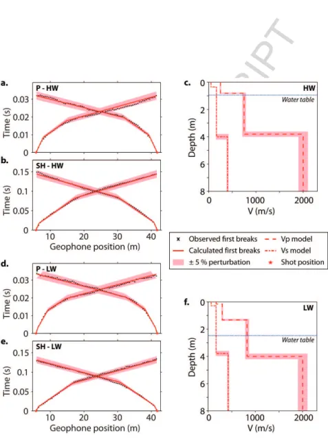
of the basin is covered with table-land loess of about 2–5 m in thickness, essentially composed of
79
sand and loam lenses of low permeability. These unconsolidated deposits seem to be connected to
80
the Oligocene sand and limestone, forming a single aquifer unit. This upper aquifer is monitored by
81
a dense network of piezometers (Fig.1a) (Mouhri et al., 2013) which have allowed for establishing
82
maps of the piezometric level for high and low water regimes in 2009 and 2011 (Kurtulus et al.,
83
2011;Kurtulus and Flipo,2012). It thus offers an ideal framework for the study of the VP/VS ratio
84
through the combined analysis of P-wave refraction, SH-wave refraction and surface-wave
disper-85
sion data. Measurements were carried out under two distinct hydrological conditions in order to
86
evaluate the ability of this approach to detect variations of the water table level, and assess its
87
practical limitations.
ACCEPTED MANUSCRIPT
2. Location of the experimentation and acquisition strategy89
2.1. Choice of the site
90
The experiment location has been selected in a plateau area, where the upper layers of the
91
aquifer system are known to be the most tabular. The site is located in the southeast part of the
92
Orgeval basin, at 70 km east from Paris, near the locality of Les Granges (black square Fig.1a).
93
A piezometer (PZ3 on Fig.1a) with its water window in the Brie aquifer is situated in the middle
94
of a trail crossing the survey area in the southeast-northwest direction. Thanks to the ORACLE
95
facilities, the piezometric head level in the upper aquifer is continuously recorded in PZ3 on an
96
hourly basis (Fig. 2a). Two acquisition campaigns were carried out in the site under two distinct
97
hydrological conditions. The first campaign took place between March 12th and March 14th 2013
98
during a high flow regime (i.e. high water level or HW on Fig.2a), with a piezometric head level
99
measured at 1.15 m. The second campaign was conducted between August 26th and August 28th
100
2013 during a low flow regime (i.e. low water level or LW on Fig.2a), with a recorded piezometric
101
head level of 2.72 m. During both HW and LW campaigns, the piezometric head level was measured
102
from ground level at the base of PZ3.
103
Electrical Resistivity Tomography was performed during both HW and LW campaigns to
accu-104
rately describe the stratigraphy in the upper aquifer unit and confirm the tabularity required for
105
our experiment. We used a multi-channel resistivimeter with a 96-electrode Wenner-Schlumberger
106
array (Fig.2b). ERT profiles were implanted on the side of the trail and centred on PZ3 (Fig.1a),
107
1 m away from the piezometer and 0.25 m below, respectively. Electrodes were spaced with 0.5 m
108
to obtain 41.5-m long profiles. The inversion was performed using the RES2DINV commercial
109
software (Loke and Barker, 1996). The origin of the depth axis in Fig. 2 and in figures hereafter
110
was chosen at ground level in the centre of the line (i.e. the water table level is 0.25 m higher
111
than recorded in PZ3). The ORACLE experimental facilities provided soil and air temperatures
112
during both campaigns thanks to probes installed near the survey area. At HW, air temperature
113
was below 0◦C and soil temperature was increasing from 6.3◦C at 0.5 m in depth to 6.5◦C at 1 m
114
in depth. In comparison, air temperature was around 22◦C at LW, with a soil temperature varying
115
from 18.5◦C at 0.5 m in depth to 18◦C at 1 m in depth. With such fluctuations between both
116
campaigns, the variation of ground resistivity due to temperature cannot be neglected. To account
117
for those effects, Campbell et al. (1949) proposed an approximation stating that an increase of
ACCEPTED MANUSCRIPT
1◦C in temperature causes a decrease of 2 % in resistivity. We used this approximation to correct
119
resistivity values obtained at HW from the temperature differences observed between HW and LW
120
periods, after extrapolating both temperature profiles in depth with an exponential trend (Oke,
121
1987). The comparison of the corrected HW ERT profile with the LW ERT profile shows no
sig-122
nificant variation of the resistivity values and clearly depicts the stratigraphy with three distinct
123
tabular layers (Fig. 2c) that are consistent with those observed at the basin scale (Fig. 1b). The
124
most superficial layer has a thickness of 0.2 to 0.25 m and an electrical resistivity (ρ) of about
125
30 Ω.m. This thin layer, corresponding to the agricultural soil, was not observed at the basin scale.
126
It presents higher resistivity values at LW that can be explained by lower water content at the
127
surface. The second layer, associated with the table-land loess, is characterised by lower
electri-128
cal resistivity values (around 12 Ω.m), with a thickness of about 3.5 m. The semi-infinite layer
129
has higher electrical resistivity values (around 35 Ω.m), and can be related to the Brie limestone
130
layer. ERT and log results offer a fine description of the site stratigraphy. These results, combined
131
with piezometric head level records, provide valuable a priori information for the interpretation of
132 seismic data. 133 2.2. Seismic acquisition 134 2.2.1. Acquisition setup 135
An identical seismic acquisition setup was deployed during both HW and LW campaigns. It
136
consisted in a simultaneous P- and surface-wave acquisition followed by a SH-wave acquisition
137
along the same line. The seismic line was centred on PZ3 (Fig.1a) along the ERT profile, with the
138
origin of the x-axis being identical to the one used for ERT (Fig.2b). While a small receiver spacing
139
is required to detect thin layers with seismic refraction, a long spread is needed for surface-wave
140
analysis in order to increase spectral resolution and investigation depth. To meet both requirements,
141
we used a dense multifold acquisition setup with 72 geophones and a 0.5 m receiver spacing to
142
obtain a 35.5-m long profile (Fig.3). We carried out a topographic leveling using a tacheometer to
143
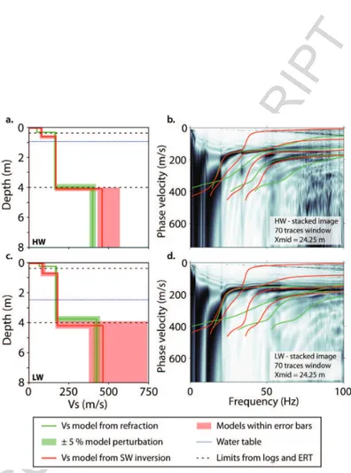
measure the relative position and elevation of each geophone. The maximum difference of elevation
144
along the profile is around 0.5 m which represent a slope of less than 1.5 %. A 72-channel seismic
145
recorder was used with 72 14-Hz vertical component geophones for the P-wave profile, and 72 14-Hz
146
horizontal component geophones for the S-wave profile. First shot location was one half receiver
147
spacing away from first trace, and move up between shots was one receiver interval. 73 shots were
ACCEPTED MANUSCRIPT
recorded along each profile for a total number of 5256 active traces.149
The P-wave source consisted in an aluminium plate hit vertically by a 7-kg sledgehammer. The
150
plate was hit 6 times at each position to increase signal-to-noise ratio. The SH-waves were generated
151
with a manual source consisting of a heavy metal frame hit laterally by a 7-kg sledgehammer. The
152
SH-wave source was hit 8 times at each position. For both P- and SH-wave acquisitions, the
153
sampling rate was 1 ms and the recording time was 2 s (anticipating low propagation velocities).
154
A delay of −0.02 s was kept before the beginning of each record to prevent early triggering issues
155
(i.e. time shift between the recording starting time and the actual beginning of the seismic signal).
156
2.2.2. Recorded seismograms
157
The collected data presented on Fig. 4 are of good quality with low noise level, and did not
158
require specific processing other than basic trace normalisation. P-wave seismograms recorded
159
during both HW (Fig. 4a) and LW (Fig. 4c) campaigns present similar characteristics. P-wave
160
first arrivals are clearly visible before 0.04 s (P on Fig.4a and 4c), with three different apparent
161
velocities visible at first glance: 200 m/s for the first two traces, then 800 m/s for the next 7
162
to 10 traces, and around 2000 m/s for the farthest traces. They are followed by the air wave,
163
characterised by higher frequencies and a velocity of 340 m/s (A on Fig.4a and4c). At last come
164
P-SV waves (or Rayleigh waves), corresponding to a high-amplitude and low-frequency wave-train
165
with an apparent velocity of about 150 m/s (R on Fig.4a and4c). SH-wave shots records obtained
166
during both HW (Fig. 4b) and LW (Fig. 4d) campaigns also show similar features. They contain
167
lower frequency signal, with coherent events consistent with SH-wave first arrivals (SH on Fig.4b
168
and4d). These first arrivals have three distinct apparent velocities (around 70 m/s for the first two
169
traces, 175 m/s for the next 30 traces, and 450 m/s for the farthest traces). SH-wave first arrivals
170
are directly followed by Love waves (L on Fig.4b and4d), which present an apparent velocity of
171
about 175 m/s. Early P-wave arrivals are visible on horizontal geophones records, especially on
172
Fig.4b between 15 and 20 m and before 0.1 s. Even under such excellent experimental conditions,
173
it is always challenging to guarantee the horizontality of geophones. These early events are one of
174
the main features that make first arrival picking delicate when carrying out SH-wave surveys.
ACCEPTED MANUSCRIPT
3. Processing and results176
3.1. Body waves
177
For both HW and LW, P- and SH-wave traveltimes were easily identified and picked in the
178
raw data from near to long offsets. First arrivals of 5 shots (1 direct shot, 1 reverse shot and
179
3 evenly spaced split-spread shots) were interpreted as simple 2D models with tabular dipping
180
layers (Wyrobek, 1956; Dobrin, 1988). Traveltimes corresponding to the interpreted models were
181
computed and represented along with observed traveltimes. In the absence of a proper estimation of
182
the traveltimes relative errors and in order to propose an estimate of the accuracy of the interpreted
183
models, we introduced a perturbation of ±5 % on interpreted models (+5 % on velocities and −5 %
184
on thicknesses for the lower model, and −5 % on velocities and +5 % on thicknesses for the upper
185
model), and calculated the corresponding theoretical traveltimes. For the sake of readability, only
186
direct and reverse shots traveltimes were represented Fig. 5 along with ±5 % perturbations. 1D
187
models corresponding to the centre of the profile (i.e. the position of PZ3) were extracted and
188
represented with the corresponding ±5 % perturbation (Fig.5).
189
P-wave first arrivals picked for the HW campaign (Fig.5a) were interpreted as a 3-layer model,
190
with interfaces between layers slightly dipping southeast (less than 1 %). These three layers have
191
P-wave velocities from surface to depth of 250 ± 12.5 m/s, 750 ± 37.5 m/s and 2000 ± 100 m/s,
192
respectively. The two upper layers have thicknesses at the centre of the profile of 0.85±0.043 m and
193
3±0.15 m, respectively (Fig.5c). P-wave first arrivals observed for the LW campaign (Fig.5d) were
194
interpreted with 4 layers presenting slightly dipping interfaces towards southeast (less than 0.5 %).
195
The corresponding velocities are 170 ± 8.5 m/s, 300 ± 15 m/s, 825 ± 41.25 m/s and 2000 ± 100 m/s
196
from top to bottom. The thicknesses of the three upper layers at the centre of the model are
197
0.15 ± 0.008 m, 1.2 ± 0.06 m and 2.65 ± 0.133 m, respectively (Fig. 5f). The first layer observed
198
during the LW campaign is missing in the interpretation of first arrivals of the HW campaign.
199
Indeed, early triggering issues prevented us from picking first arrivals corresponding to this thin
200
layer.
201
SH-wave first arrivals picked for both HW (Fig. 5b) and LW (Fig. 5e) campaigns were
inter-202
preted as 3-layer models, with interfaces slightly dipping southeast (less than 0.25 %). For HW,
203
these three layers are characterised from top to bottom by SH-wave velocities of 50 ± 2.5 m/s,
204
165 ± 8.25 m/s and 400 ± 20 m/s, respectively. The two upper layers are 0.35 ± 0.018 m and
ACCEPTED MANUSCRIPT
3.65 ± 0.183 m thick, respectively (Fig. 5c). As for LW, the VS model at the centre of the
pro-206
file is composed of a low velocity (65 ± 3.25 m/s) and thin (0.3 ± 0.015 m) layer in surface, a
207
3.5 ± 0.175 m thick layer with a velocity of 170 ± 8.5 m/s, and a semi-infinite layer with a velocity
208
of 425 ± 21.25 m/s (Fig.5f).
209
Despite known limitations of the refraction interpretation technique (e.g. in presence of low
210
velocity layers, velocity gradients, etc.), the interpreted velocity models are highly satisfying and
211
provide a description of the stratigraphy in very good agreement with ERT and log results. When
212
VS show 3 layers corresponding to this stratigraphy, VP present a fourth layer that is consistent
213
with the observed water table level, especially for HW (Fig. 5c). These velocity models are quite
214
stable in depth, as demonstrated by the ±5 % error bars displayed on Fig. 5. Furthermore, the
215
calculated residuals between observed and calculated traveltimes remain mostly below 5 %, with
216
only a few over 10 %, and Root Mean Square (RMS) errors calculated for direct and reverse shots
217
are around 2-2.5 % (Fig. 6). These low values point out the good consistency of the estimated
218
velocity models and reinforce the confidence in our interpretations.
219
3.2. P-SV waves
220
3.2.1. Extraction of dispersion
221
Surface-wave dispersion images were obtained from P-wave shot gathers for both HW and
222
LW campaigns (Fig. 7). After correction for geometrical spreading, the wavefield was basically
223
transformed to the frequency-phase velocity (f − c) domain in which maxima should correspond to
224
Rayleigh-wave propagation modes (Russel,1987;Mokhtar et al.,1988). Anticipating slight shallow
225
lateral variations, we used the entire spread to analyse surface waves. A 70-trace extraction window
226
(34.5-m wide) was actually used in order to be roughly centred on PZ3 (x = 24.25 m). For both flow
227
regimes, we obtained dispersion images from direct (Fig.7a, HW and7d, LW) and reverse (Fig.7b,
228
HW and7e, LW) shots on each side of the window. The comparison of both single dispersion images
229
presented only slight differences, confirming the validity of the 1D approximation (Jongmans et al.,
230
2009). These images were thus stacked in order to increase the signal-to-noise ratio (Fig.7c, HW and
231
7f, LW). The stacking was achieved by summing the frequency-phase velocity spectra of windowed
232
data (e.g.O’Neill et al.,2003), which clearly enhanced the maxima.
233
The dispersion data present a strong “effective character”, which aspects are for instance
dis-234
cussed by Forbriger (2003a,b) and O’Neill and Matsuoka (2005). In shallow seismic data, large
ACCEPTED MANUSCRIPT
velocity contrasts and/or velocity gradients often generate wavefields with dominant higher modes.
236
Guided waves may also appear with large amplitudes at high frequencies and phase velocities. In
237
that case, the identification of different propagation modes and the picking of dispersion curves
238
is challenging and requires a thorough analysis of the observed dispersion images, or alternative
239
inversion approaches (e.g.Maraschini et al., 2010; Boiero et al., 2013). To facilitate mode
identifi-240
cation, we relied on preliminary picking and inversions along with trial and error forward modelling
241
based on a priori geological knowledge and results from refraction analysis. Such approach
actu-242
ally highlighted a “mode-jump” occurring around 35 Hz on each dispersion image, confirming the
243
presence of overlapping modes. Some maxima yet remained hard to identify as propagation modes
244
in the extracted dispersion images, either because they could be seen as secondary lobes of the
245
wavefield transform, or because they were too close to other maxima. To prevent from including
246
“misidentified modes” in dispersion data, maxima were not picked in those areas.
247
On each dispersion image, coherent maxima were finally extracted with an estimated standard
248
error in phase velocity defined according to the workflow described inO’Neill(2003). Corresponding
249
error bars are not presented on Fig. 7 to keep images readable. Four propagation modes were
250
observed and identified as fundamental (0), first (1), second (2) and third (3) higher modes (Fig.7).
251
The apparent phase velocity of the fundamental mode increases with decreasing frequency (from
252
175 to 350 m/s). As recommended byBodet (2005) andBodet et al.(2009), we limited dispersion
253
curves down to frequencies (flim) where the spectral amplitude of the seismogram became too low
254
(15 Hz on Fig.7), thus defining the maximum observed wavelength λmax (∼ 22.5 m on Fig.7).
255
3.2.2. Inversion
256
Assuming a 1D tabular medium below each extraction window, we performed a 1D inversion
257
of dispersion data obtained during both HW and LW campaigns. We used the Neighbourhood
258
Algorithm (NA) developed bySambridge(1999) and implemented for near-surface applications by
259
Wathelet et al. (2004) and Wathelet (2008). Theoretical dispersion curves were computed from
260
the elastic parameters using the Thomson-Haskell matrix propagator technique (Thomson, 1950;
261
Haskell, 1953). NA performs a stochastic search of a pre-defined parameter space (namely VP, VS,
ACCEPTED MANUSCRIPT
density and thickness of each layer), using the following misfit function (MF ):263 M F = v u u t Nf X i=1 (Vcali− Vobsi) 2 Nfσi2 , (1)
with Vcali and Vobsi, the calculated and observed phase velocities at each frequency fi; Nf, the 264
number of frequency samples and σi, the phase velocity measurement error at each frequency fi.
265
Based on site a priori geological knowledge and results from refraction analysis, we used a
266
parametrisation with a stack of three layers (soil, partially saturated loess and fully saturated
267
loess) with an uniform velocity distribution overlaying the half-space (Brie limestone layer). An
268
appropriate choice of these parameters is considered as a fundamental issue for the successful
269
application of inversion (Socco and Strobbia, 2004; Renalier et al., 2010). The thickness of the
270
soil layer was allowed for ranging from 0.05 to 1 m, while the thicknesses of the partially and
271
fully saturated loess could vary between 0.5 and 3.5 m. The half-space depth (HSD), of great
272
importance since it depends on the poorly known depth of investigation of the method, was fixed
273
to about 40 % of the maximum observed wavelength (8 m) as recommended by O’Neill (2003)
274
and Bodet et al. (2005, 2009). The valid parameter range for sampling velocity models was 1 to
275
750 m/s for VS (based on dispersion observations and refraction analysis). Anticipating a decrease
276
of VS in the saturated zone, we did not constraint velocities to increase with depth in the two
277
layers corresponding to the partially and fully saturated loess, as it is usually done in surface-wave
278
methods (Wathelet, 2008). P-wave velocity being of weak contraint on surface-wave dispersion,
279
only S-wave velocity profile can be interpreted. VP however remain part of the actual parameter
280
space and were generated in the range 10 to 2500 m/s. Density was set as uniform (1800 kg/m3).
281
A total of 75300 models were generated with NA (Fig. 8a, HW and 8c, LW). Models matching
282
the observed data within the error bars were selected, as suggested by Endrun et al.(2008). The
283
accepted models were used to build a final average velocity model associated with the centre of the
284
extraction window (dashed line Fig. 8b, HW and 8d, LW). Thickness and velocity accuracy was
285
estimated with the envelope containing the accepted models.
286
For both HW (Fig.8b) and LW (Fig.8d) campaigns, the inversion led to very similar 4-layer
287
VS models. While velocities in the second and third layers were not constrained to increase with
288
depth, neither final VS model presents decreasing velocities. These two models are characterised
289
by the same very thin low velocity layer in surface (around 0.052 ± 0.025 m in thickness with a
ACCEPTED MANUSCRIPT
S-wave velocity of 8 ± 3 m/s). The second layer is slightly thicker for LW (0.67 ± 0.14 m) than for
291
HW (0.56 ± 0.11 m), and has higher VS values for LW (86 ± 15 m/s) than for HW (79 ± 10 m/s).
292
The third layer has identical thickness for both flow regimes (3.47 ± 0.25 m), but VS is slighlty
293
higher for LW (179 ± 10 m/s) than for HW (169 ± 5 m/s). The half-space is also characterised by
294
very similar velocities for both flow regimes, with 459 m/s for HW (between 430 and 570 m/s),
295
and 464 m/s for LW (between 380 and 740 m/s). Dispersion curves being less well defined at low
296
frequencies, a larger variability (i.e. larger error bars) of half-space velocities is observed, especially
297
for LW.
298
This first layer is actually very thin and “slow” but was identified on the field and corresponds
299
to a “mode-jump” in the fundamental mode at about 35 Hz. The high frequency part of this
300
mode could not be picked on dispersion images (Fig. 7) due to stronger higher modes above that
301
frequency, and was thus not included as a priori information in our parameterisation. Using only
302
the fundamental mode in the inversion would obviously have given different results, with theoretical
303
dispersion curves not necessarily presenting this ”mode-jump“. The incorporation of higher modes
304
in the inversion process allowed us to constrain the fundamental mode behavior at high frequency,
305
even though we could not identify it above 35 Hz. Indeed, all models included within the error
306
bars (Fig.8) present the same ”mode-jump“ at frequencies higher than 35 Hz, leading to velocity
307
models with a thin low velocity layer at the surface.
308
3.3. Cross-validation ofVS models
309
Models obtained from surface-wave dispersion inversion (in red, Fig. 9a for HW and 9c for
310
LW) are remarkably similar to the models obtained from SH-wave refraction interpretation (in
311
green, Fig.9a for HW and9c for LW), and are thus very consistent with the stratigraphy observed
312
on ERT and log results (Fig.2). VS obtained through surface-wave dispersion inversion are
how-313
ever characterised for both flow regimes by a very thin and low velocity layer in surface that is
314
not observed with SH-wave refraction interpretation. The error bars of VS models retrieved from
315
refraction analysis were estimated by introducing a perturbation of ±5 % on the central model
316
parameters (in green, Fig. 9a for HW and 9c for LW). As for error bars of VS models retrieved
317
from surface-wave dispersion inversion (in red, Fig.9a for HW and9c for LW), they correspond to
318
the envelope of accepted models for each hydrological regime (i.e. fitting the error bars in Fig.8).
319
As a final quality control of inversion results, forward modelling was performed using the 1D
ACCEPTED MANUSCRIPT
VS average models obtained from both surface-wave dispersion inversion and SH-wave refraction
321
interpretation. While models obtained from both methods are remarkably similar, the
theoreti-322
cal dispersion curves computed from surface-wave dispersion inversion results (in red, Fig. 9b for
323
HW and 9d for LW) provide the best fit with the coherent maxima observed on measured
dis-324
persion images. The theoretical modes are consistent with the picked dispersion curves, and are
325
well-separated from each other while they looked like a unique and strong mode at first glance.
326
Interestingly, theoretical dispersion curves calculated from refraction models (in green, Fig.9a for
327
HW and 9c for LW) are clearly following this effective dispersion which remains representative
328
of the stratigraphy since models from both methods are in good agreement. There is however no
329
evidence of water table level detection, though several authors noticed a significant VS velocity
330
decrease in the saturated zone (O’Neill and Matsuoka,2005;Heitor et al.,2012).
331
4. Discussion and conclusions
332
When studying aquifer systems, hydrogeologists mainly rely on piezometric and log data to
333
estimate the spatial variations of water table level and lithology. However, these data provide only
334
local information and require the implantation of boreholes which remain expensive and destructive.
335
Geophysical methods are increasingly proposed to interpolate this piezometric and lithological
336
information between boreholes and build high resolution hydrological models. If electrical and
337
electromagnetic methods have shown their efficiency for the fine characterisation of the lithology,
338
they remained nonetheless unable to detect the water table level in clayey geological formations such
339
as loess. In order to assess the ability of seismic methods to retrieve water table level variations,
340
we carried out seismic measurements in a site characterised by a tabular aquifer system,
well-341
delineated thanks to ERT, log and piezometer data. Measurements were completed under two
342
distinct hydrological conditions (HW and LW). A simultaneous P- and surface-wave survey was
343
achieved with a single acquisition setup, followed by a SH-wave acquisition along the same line.
344
A simple refraction interpretation of P- and SH-wave first arrivals provided quasi-1D VP and VS
345
models in conformity with the stratigraphy depicted by ERT and logs during both campaigns. VS
346
models obtained through surface-wave dispersion inversion are matching those obtained with
SH-347
wave refraction interpretation, except for a thin low velocity layer in surface, which has only been
348
identified in surface-wave dispersion inversion results. The recomputation of theoretical dispersion
ACCEPTED MANUSCRIPT
curves provided results that are very consistent with the measured dispersion images and proved to
350
be a reliable tool for validating the 1D VS models obtained from SH-wave refraction interpretation
351
and surface-wave dispersion inversion.
352
While VS remains constant in partially and fully saturated loess, VP exhibits a strong increase
353
at a depth consistent with the observed water table level, especially for HW. This correlation is
354
yet not so obvious for LW. Furthermore, VP values observed in the saturated loess remain lower
355
(around 800 m/s) than the expected values in fully saturated sediments (usually around
1500-356
1600 m/s). It is however quite hard to find in the literature a range of typical VP values that
357
should be expected in various partially and fully saturated sediments. Most of the existing studies
358
present VP values in saturated sands, where the relationship between VP and water saturation
359
remains quite simple and is thoroughly described by many authors (e.g.Bachrach et al.,2000;Foti
360
et al.,2002;Prasad,2002;Zimmer et al.,2007a,b). With more complex mixtures (e.g. containing a
361
significant proportion of clays), the behavior of VP with the saturation becomes more complicated
362
(Fratta et al., 2005). VP values around 800 m/s have already been observed in saturated loess
363
by Danneels et al.(2008) when studying unstable slopes in Kyrgyzstan. In such low permeability
364
materials, full saturation can be hard to reach (due to an irreducible fraction of air in the pores),
365
thus limiting the maximum VP velocity (Lu and Sabatier, 2009; Lorenzo et al., 2013). The study
366
of VP alone thus remains insufficient to lead back to hydrological information. In order to cope
367
with this limitation, VP/VS (Fig.10a for HW,10c for LW) and Poisson’s ratios (Fig.10b for HW,
368
10d for LW) were computed with VS models retrieved from SH-wave refraction interpretation (in
369
green) and surface-wave dispersion inversion (in red). In any case, VP/VS and Poisson’s ratios were
370
computed with VP retrieved from P-wave refraction interpretation.
371
For HW, VP/VS ratio (Fig. 10a) is around 4 in the soil layer, and Poisson’s ratio (Fig. 10b)
372
ranges between 0.45 and 0.48. These values are typical of saturated soils (Uyanık,2011), and may be
373
explained by the presence of a melting snow cover on the site during the acquisition. Directly down
374
the soil, the loess layer is characterised down to 0.75-0.85-m deep by VP/VS ratio values of 1.5 and
375
Poisson’s ratio values of 0.1. These values are unusually low, even for non-saturated sediments, and
376
might be explained by the presence of a frozen layer (Wang et al.,2006). At this depth, consistent
377
with the water table level (0.9 m), VP/VS and Poisson’s ratios values increase to 4.5 and 0.47-0.48,
378
respectively. This kind of contrast in a single lithological unit is typical of a transition between
ACCEPTED MANUSCRIPT
partially saturated (low VP/VS and Poisson’s ratios) and fully saturated sediments (high VP/VS
380
and Poisson’s ratios). VP/VS and Poisson’s ratios remain constant in the deepest part of loess
381
and in the Brie limestone layer, reinforcing the assumption of a continuously saturated aquifer. A
382
similar contrast is visible for LW on VP/VS (Fig. 10c) and Poisson’s (Fig. 10d) ratios. The depth
383
of this contrast (between 1.25 and 1.40 m) is not in very good agreement with the water table level
384
(2.47 m), but yet do not correspond to any stratigraphic limit. The low VP/VS and Poisson’s ratios
385
values (around 1.7 and 0.24, respectively) in the upper part of the loess support the assumption of
386
a partially saturated area, while the high values of these ratios (around 4.5 and 0.48, respectively)
387
computed in the deepest part of the loess and in the Brie limestone layer are consitent with a fully
388
saturated porous medium.
389
These results are supported by water content measurements performed on auger sounding
390
samples collected during the LW campaign (soil samples could not be collected during the HW
391
campaign due to unfavorable weather conditions). As can be observed on Fig. 10e, the water
392
content decreases between the soil and the upper part of the loess, and reaches a minimum around
393
0.8-0.9 m. Between 1.2 and 1.5 m, a small peak of moisture is observed, probably corresponding
394
to a rainfall event that occurred 24 hours before the sounding (pluviometry data are available at
395
http://bdoracle.irstea.fr/). This peak is followed by a progressive increase of water content
396
that reaches a maximum at a depth corresponding to the water table level. Auger refusal was
397
encountered at 2.70 m, thus limiting the number of measurements in the saturated zone. The
398
differences observed for LW between the water table level and the depth of the contrast of VP/VS
399
and Poisson’s ratios can be explained by several mechanisms. In near-surface sediments, capillary
400
forces create a saturated zone above the water table (Lu and Likos, 2004; Lorenzo et al., 2013)
401
that can reach up to 60 cm in such silty sediments (Lu and Likos, 2004). Refraction probably
402
occurs above the water table on this capillarity fringe. The rainfall event observed on Fig. 10
403
might have a similar effect, since the depth of the peak of moisture corresponds to the depth at
404
which the VP/VS contrast occurs. The decrease of water content between the rainfall peak and
405
the water table probably creates a low velocity zone that alters the first arrivals interpretation
406
(irrespective of the acquisition configuration). The relevance of this tabular interpretation might
407
be called into question if the studied medium is characterised by continuously varying properties
408
with velocities increasing progressively from the partially saturated area to the fully saturated
ACCEPTED MANUSCRIPT
area (Cho and Santamarina, 2001). Despite an advanced and thorough analysis of surface-wave
410
dispersion, no decrease of VS is detected in the fully saturated zone. This is probably due to very
411
weak variations of water content between the partially and fully saturated areas (Fig.10e), which do
412
not produce a significant decrease of VS in such material (Dhemaied et al.,2014). Such issues have
413
to be adressed thanks to laboratory experiments by combining analogue modelling and ultrasonic
414
techniques (Bergamo et al.,2014; Bodet et al.,2014) on water saturated porous media (Pasquet,
415
2014). Despite these theoretical issues, our approach provided encouraging results that call for
416
more experimental validation. Furthermore, the use of single acquisition setup to retrieve both
417
VP and VS from refraction interpretation and surface-wave analysis appears promising in terms
418
of acquisition time and costs. Associated with existing piezometric data, seismic measurements
419
could be carried out at a wider scale throughout the entire basin to build high resolution maps of
420
the piezometric level. Its application in more complex (e.g. 2D) cases should also provide valuable
421
information for the study of stream-aquifer interactions.
422
5. Acknowledgments
423
This work was supported by the french national programme EC2CO – Biohefect (project
424
“´Etudes exp´erimentales multi-´echelles de l’apport des vitesses sismiques `a la description du
contin-425
uum sol-aquif`ere”). It was also supported by the ONEMA NAPROM project and the workpackage
426
“Stream-Aquifer Interfaces” of the PIREN Seine research program. It is a contribution to the GIS
427
ORACLE (Observatoire de Recherche sur les bassins versants ruraux Am´enag´es, pour les Crues,
428
Les ´Etiages et la qualit´e de l’eau) that maintains the experimental facilities of the Orgeval basin.
429
We kindly thank P. Ansart (IRSTEA) for technical assistance and logistic support during field
430
work.
ACCEPTED MANUSCRIPT
6. References432
Adam, L., Batzle, M., Brevik, I., 2006. Gassmann’s fluid substitution and shear modulus variability in carbonates
433
at laboratory seismic and ultrasonic frequencies. Geophysics 71(6), F173–F183.
434
Bachrach, R., Dvorkin, J., Nur, A., 2000. Seismic velocities and Poisson’s ratio of shallow unconsolidated sands.
435
Geophysics 65(2), 559–564.
436
Bachrach, R., Nur, A., 1998. High-resolution shallow-seismic experiments in sand, Part I: Water table, fluid flow,
437
and saturation. Geophysics 63(4), 1225–1233.
438
Bates, C.R., Phillips, D., Hild, J., 1992. Studies in P-wave and S-wave seismics, in: Symposium on the Application
439
of Geophysics to Engineering and Environmental Problems, EEGS, Oakbrook, Illinois, USA.
440
Bergamo, P., Bodet, L., Socco, L.V., Mourgues, R., Tournat, V., 2014. Physical modelling of a surface-wave survey
441
over a laterally varying granular medium with property contrasts and velocity gradients. Geophysical Journal
442
International 197(1), 233–247.
443
Berryman, J.G., 1999. Origin of Gassmann’s equations. Geophysics 64(5), 1627–1629.
444
Biot, M.A., 1956a. Theory of propagation of elastic waves in a fluid-saturated porous solid. I. Low-frequency range.
445
The Journal of the Acoustical Society of America 28(2), 168–178.
446
Biot, M.A., 1956b. Theory of propagation of elastic waves in a fluid-saturated porous solid. II. Higher frequency
447
range. The Journal of the Acoustical Society of America 28(2), 179–191.
448
Bodet, L., 2005. Limites th´eoriques et exp´erimentales de l’interpr´etation de la dispersion des ondes de Rayleigh :
449
apport de la mod´elisation num´erique et physique. Ph.D. thesis. ´Ecole Centrale de Nantes et Universit´e de Nantes.
450
Nantes, France.
451
Bodet, L., Abraham, O., Clorennec, D., 2009.Near-offset effects on Rayleigh-wave dispersion measurements: Physical
452
modeling. Journal of Applied Geophysics 68(1), 95–103.
453
Bodet, L., Dhemaied, A., Martin, R., Mourgues, R., Rejiba, F., Tournat, V., 2014. Small-scale physical modeling of
454
seismic-wave propagation using unconsolidated granular media. Geophysics 79(6), T323–T339.
455
Bodet, L., van Wijk, K., Bitri, A., Abraham, O., Cˆote, P., Grandjean, G., Leparoux, D., 2005.Surface-wave inversion
456
limitations from laser-Doppler physical modeling. Journal of Environmental and Engineering Geophysics 10(2),
457
151–162.
458
Boiero, D., Wiarda, E., Vermeer, P., 2013. Surface- and guided-wave inversion for near-surface modeling in land and
459
shallow marine seismic data. The Leading Edge 32(6), 638–646.
460
Bradford, J.H., 2002.Depth characterization of shallow aquifers with seismic reflection, Part I—The failure of NMO
461
velocity analysis and quantitative error prediction. Geophysics 67(1), 89–97.
462
Bradford, J.H., Sawyer, D.S., 2002. Depth characterization of shallow aquifers with seismic reflection, Part
463
II—Prestack depth migration and field examples. Geophysics 67(1), 98–109.
464
Cameron, A., Knapp, C., 2009. A new approach to predict hydrogeological parameters using shear waves from
465
multichannel analysis of surface waves method, in: Symposium on the Application of Geophysics to Engineering
466
and Environmental Problems, EEGS, Fort Worth, Texas, USA.
467
Campbell, R.B., Bower, C.A., Richards, L.A., 1949. Change of electrical conductivity with temperature and the
ACCEPTED MANUSCRIPT
relation of osmotic pressure to electrical conductivity and ion concentration for soil extracts. Soil Science Society
469
of America Journal 13, 66–69.
470
Castagna, J.P., Amato, M., Eastwood, R., 1985.Relationships between compressional-wave and shear-wave velocities
471
in clastic silicate rocks. Geophysics 50(4), 571–581.
472
Cho, G.C., Santamarina, J.C., 2001.Unsaturated particulate materials - particle-level studies. Journal of Geotechnical
473
and Geoenvironmental Engineering 127(1), 84–96.
474
Dal Moro, G., Keller, L., 2013. Unambiguous determination of the Vs profile via joint analysis of multi-component
475
active and passive seismic data, in: Near Surface Geoscience 2013 – 19th European Meeting of Environmental and
476
Engineering Geophysics, EAGE, Bochum, Germany.
477
Danneels, G., Bourdeau, C., Torgoev, I., Havenith, H.B., 2008.Geophysical investigation and dynamic modelling of
478
unstable slopes: case-study of Kainama (Kyrgyzstan). Geophysical Journal International 175(1), 17–34.
479
Dhemaied, A., Cui, Y.J., Tang, A.M., Nebieridze, S., Terpereau, J.M., Leroux, P., 2014. Effet de l’´etat hydrique sur
480
la raideur m´ecanique, in: GEORAIL 2014, 2`eme Symposium International en G´eotechnique Ferroviaire,
Marne-481
la-Vall´ee, France.
482
Dobrin, M.B., 1988. Introduction to geophysical prospecting. 4 ed., McGraw-Hill Book Co.
483
Domenico, S.N., 1974.Effect of water saturation on seismic reflectivity of sand reservoirs encased in shale. Geophysics
484
39(6), 759–769.
485
Domenico, S.N., 1977. Elastic properties of unconsolidated porous sand reservoirs. Geophysics 42(7), 1339–1368.
486
Dvorkin, J., 2008.Yet another Vs equation. Geophysics 73(2), E35–E39.
487
Dvorkin, J., Nur, A., 1998. Acoustic signatures of patchy saturation. International Journal of Solids and Structures
488
35(34–35), 4803–4810.
489
Endrun, B., Meier, T., Lebedev, S., Bohnhoff, M., Stavrakakis, G., Harjes, H.P., 2008.S velocity structure and radial
490
anisotropy in the Aegean region from surface wave dispersion. Geophysical Journal International 174(2), 593–616.
491
Fabien-Ouellet, G., Fortier, R., 2014. Using all seismic arrivals in shallow seismic investigations. Journal of Applied
492
Geophysics 103, 31–42.
493
Flipo, N., Rejiba, F., Kurtulus, B., Tournebize, J., Tallec, G., Vilain, G., Garnier, J., Ansart, P., Lotteau, M., 2009.
494
Caract´erisation des fonctionnements hydrologique et hydrog´eologiques du bassin de l’Orgeval. Technical Report.
495
PIREN Seine.
496
Forbriger, T., 2003a. Inversion of shallow-seismic wavefields: I. Wavefield transformation. Geophysical Journal
497
International 153(3), 719–734.
498
Forbriger, T., 2003b.Inversion of shallow-seismic wavefields: II. Inferring subsurface properties from wavefield
trans-499
forms. Geophysical Journal International 153(3), 735–752.
500
Foti, S., Lancellotta, R., Lai, C.G., 2002. Porosity of fluid-saturated porous media from measured seismic wave
501
velocities. G´eotechnique 52(5), 359–373.
502
Fratta, D., Alshibli, K.A., Tanner, W., Roussel, L., 2005.Combined TDR and P-wave velocity measurements for the
503
determination of in situ soil density—experimental study. Geotechnical Testing Journal 28(6), 12293.
504
Gabriels, P., Snieder, R., Nolet, G., 1987.In situ measurements of shear-wave velocity in sediments with higher-mode
505
Rayleigh waves. Geophysical Prospecting 35(2), 187–196.
ACCEPTED MANUSCRIPT
Gaines, D., Baker, G.S., Hubbard, S.S., Watson, D., Brooks, S., Jardine, P., 2010. Detecting perched water bodies
507
using surface-seismic time-lapse traveltime tomography, in: Advances in Near-surface Seismology and
Ground-508
penetrating Radar. Society of Exploration Geophysicists, American Geophysical Union, Environmental and
Engi-509
neering Geophysical Society, pp. 415–428.
510
Galibert, P.Y., Valois, R., Mendes, M., Gu´erin, R., 2014. Seismic study of the low-permeability volume in southern
511
France karst systems. Geophysics 79(1), EN1–EN13.
512
Ghasemzadeh, H., Abounouri, A.A., 2012. Effect of subsurface hydrological properties on velocity and attenuation
513
of compressional and shear wave in fluid-saturated viscoelastic porous media. Journal of Hydrology 460–461,
514
110–116.
515
Ghose, R., Carvalho, J., Loureiro, A., 2013. Signature of fault zone deformation in near-surface soil visible in shear
516
wave seismic reflections. Geophysical Research Letters 40(6), 1074–1078.
517
Gregory, A.R., 1976.Fluid saturation effects on dynamic elastic properties of sedimentary rocks. Geophysics 41(5),
518
895–921.
519
Grelle, G., Guadagno, F.M., 2009. Seismic refraction methodology for groundwater level determination: “Water
520
seismic index”. Journal of Applied Geophysics 68(3), 301–320.
521
Gu´erin, R., 2005. Borehole and surface-based hydrogeophysics. Hydrogeology Journal 13(1), 251–254.
522
Guy, E.D., Nolen-Hoeksema, R.C., Daniels, J.J., Lefchik, T., 2003.High-resolution SH-wave seismic reflection
inves-523
tigations near a coal mine-related roadway collapse feature. Journal of Applied Geophysics 54(1–2), 51–70.
524
Haeni, F.P., 1986a.Application of continuous seismic reflection methods to hydrologic studies. Ground Water 24(1),
525
23–31.
526
Haeni, F.P., 1986b. Application of seismic refraction methods in groundwater modeling studies in New England.
527
Geophysics 51(2), 236–249.
528
Haeni, F.P., 1988. Application of seismic-refraction techniques to hydrologic studies. Technical Report TWRI
-529
02-D2. United States Geological Survey.
530
Haines, S.S., 2007.A hammer-impact, aluminium, shear-wave seismic source. Technical Report OF 07-1406. United
531
States Geological Survey.
532
Haines, S.S., Ellefsen, K.J., 2010. Shear-wave seismic reflection studies of unconsolidated sediments in the near
533
surface. Geophysics 75(2), B59–B66.
534
Haines, S.S., Pidlisecky, A., Knight, R., 2009. Hydrogeologic structure underlying a recharge pond delineated with
535
shear-wave seismic reflection and cone penetrometer data. Near Surface Geophysics 7(5-6), 329–339.
536
Haskell, N.A., 1953.The dispersion of surface waves on multilayered media. Bulletin of the Seismological Society of
537
America 43(1), 17–34.
538
Heitor, A., Indraratna, B., Rujikiatkamjorn, C., Golaszewski, R., 2012. Characterising compacted fills at Penrith
539
Lakes development site using shear wave velocity and matric suction, in: 11th Australia - New Zealand Conference
540
on Geomechanics: Ground Engineering in a Changing World, Melbourne, Australia.
541
Hubbard, S.S., Linde, N., 2011.Hydrogeophysics, in: Treatise on Water Science. Elsevier, pp. 401–434.
542
Hunter, J.A., Benjumea, B., Harris, J.B., Miller, R.D., Pullan, S.E., Burns, R.A., Good, R.L., 2002. Surface and
543
downhole shear wave seismic methods for thick soil site investigations. Soil Dynamics and Earthquake Engineering
ACCEPTED MANUSCRIPT
22(9–12), 931–941.
545
Jongmans, D., Bi`evre, G., Renalier, F., Schwartz, S., Beaurez, N., Orengo, Y., 2009. Geophysical investigation of a
546
large landslide in glaciolacustrine clays in the Tri`eves area (French Alps). Engineering Geology 109(1–2), 45–56.
547
Jongmans, D., Demanet, D., 1993.The importance of surface waves in vibration study and the use of Rayleigh waves
548
for estimating the dynamic characteristics of soils. Engineering Geology 34(1–2), 105–113.
549
Juhlin, C., Palm, H., M¨ullern, C.F., W˚allberg, B., 2000. High-resolution reflection seismics applied to detection of
550
groundwater resources in glacial deposits, Sweden. Geophysical Research Letters 27(11), 1575–1578.
551
Kaiser, A.E., Green, A.G., Campbell, F.M., Horstmeyer, H., Manukyan, E., Langridge, R.M., McClymont, A.F.,
552
Mancktelow, N., Finnemore, M., Nobes, D.C., 2009. Ultrahigh-resolution seismic reflection imaging of the Alpine
553
Fault, New Zealand. Journal of Geophysical Research: Solid Earth 114(B11), B11306.
554
King, M.S., 1966. Wave velocities in rocks as a function of change in overburden pressure and pore fluid saturants.
555
Geophysics 31(1), 50–73.
556
Konstantaki, L.A., Carpentier, S.F.A., Garofalo, F., Bergamo, P., Socco, L.V., 2013. Determining hydrological and
557
soil mechanical parameters from multichannel surface-wave analysis across the Alpine Fault at Inchbonnie, New
558
Zealand. Near Surface Geophysics 11(4), 435–448.
559
Kurtulus, B., Flipo, N., 2012. Hydraulic head interpolation using anfis—model selection and sensitivity analysis.
560
Computers & Geosciences 38(1), 43–51.
561
Kurtulus, B., Flipo, N., Goblet, P., Vilain, G., Tournebize, J., Tallec, G., 2011. Hydraulic head interpolation in an
562
aquifer unit using ANFIS and Ordinary Kriging. Studies in Computational Intelligence 343, 265–276.
563
Lee, M.W., 2002.Modified Biot-Gassmann theory for calculating elastic velocities for unconsolidated and consolidated
564
sediments. Marine Geophysical Researches 23(5-6), 403–412.
565
Liberty, L.M., Clement, W.P., Knoll, M.D., 1999. Surface and borehole seismic characterization of the boise
hy-566
drogeophysical research site, in: Symposium on the Application of Geophysics to Engineering and Environmental
567
Problems, EEGS, Oakland, California, USA.
568
Loke, M.H., Barker, R.D., 1996. Rapid least-squares inversion of apparent resistivity pseudosections by a
quasi-569
Newton method. Geophysical Prospecting 44(1), 131–152.
570
Lorenzo, J.M., Smolkin, D.E., White, C., Chollett, S.R., Sun, T., 2013. Benchmark hydrogeophysical data from a
571
physical seismic model. Computers & Geosciences 50, 44–51.
572
Lu, N., Likos, W.J., 2004. Unsaturated soil mechanics. John Wiley & Sons.
573
Lu, Z., Sabatier, J.M., 2009.Effects of soil water potential and moisture content on sound speed. Soil Science Society
574
of America Journal 73(5), 1614–1625.
575
Maraschini, M., Ernst, F., Foti, S., Socco, L.V., 2010. A new misfit function for multimodal inversion of surface
576
waves. Geophysics 75(4), G31–G43.
577
McClymont, A.F., Roy, J.W., Hayashi, M., Bentley, L.R., Maurer, H., Langston, G., 2011.Investigating groundwater
578
flow paths within proglacial moraine using multiple geophysical methods. Journal of Hydrology 399(1–2), 57–69.
579
Michot, D., Benderitter, Y., Dorigny, A., Nicoullaud, B., King, D., Tabbagh, A., 2003. Spatial and temporal
moni-580
toring of soil water content with an irrigated corn crop cover using surface electrical resistivity tomography. Water
581
Resources Research 39(5), 1138.
ACCEPTED MANUSCRIPT
Mokhtar, T.A., Herrmann, R.B., Russell, D.R., 1988.Seismic velocity and Q model for the shallow structure of the
583
Arabian Shield from short-period Rayleigh waves. Geophysics 53(11), 1379–1387.
584
Mota, R., Monteiro Santos, F.A., 2010. 2D sections of porosity and water saturation from integrated resistivity and
585
seismic surveys. Near Surface Geophysics 8(6), 575–584.
586
Mouhri, A., Flipo, N., Rejiba, F., de Fouquet, C., Bodet, L., Kurtulus, B., Tallec, G., Durand, V., Jost, A., Ansart,
587
P., Goblet, P., 2013.Designing a multi-scale sampling system of stream–aquifer interfaces in a sedimentary basin.
588
Journal of Hydrology 504, 194–206.
589
Murphy, W.F., 1982. Effects of partial water saturation on attenuation in Massilon sandstone and Vycor porous
590
glass. The Journal of the Acoustical Society of America 71(6), 1458–1468.
591
Nur, A., Simmons, G., 1969.The effect of saturation on velocity in low porosity rocks. Earth and Planetary Science
592
Letters 7(2), 183–193.
593
Oke, T.R., 1987. Boundary layer climates. Taylor & Francis.
594
O’Neill, A., 2003. Full-waveform reflectivity for modelling, inversion and appraisal of seismic surface wave dispersion
595
in shallow site investigations. Ph.D. thesis. University of Western Australia. Perth, Australia.
596
O’Neill, A., Dentith, M., List, R., 2003. Full-waveform P-SV reflectivity inversion of surface waves for shallow
597
engineering applications. Exploration Geophysics 34(3), 158–173.
598
O’Neill, A., Matsuoka, T., 2005. Dominant higher surface-wave modes and possible inversion pitfalls. Journal of
599
Environmental and Engineering Geophysics 10(2), 185–201.
600
Paillet, F.L., 1995. Integrating surface geophysics, well logs and hydraulic test data in the characterization of
601
heterogeneous aquifers. Journal of Environmental and Engineering Geophysics 1(1), 1–13.
602
Park, C.B., Miller, R.D., Xia, J., 1999.Multichannel analysis of surface waves. Geophysics 64(3), 800–808.
603
Pasquet, S., 2014. Apport des m´ethodes sismiques `a l’hydrog´eophysique : importance du rapport Vp/Vs et
contri-604
bution des ondes de surface. Ph.D. thesis. Universit´e Pierre et Marie Curie. Paris, France.
605
Pasquet, S., Sauvin, G., Andriamboavonjy, M.R., Bodet, L., Lecomte, I., Gu´erin, R., 2014. Surface-wave dispersion
606
inversion versus SH-wave refraction tomography in saturated and poorly dispersive quick clays, in: Near Surface
607
Geoscience 2014 – 20th European Meeting of Environmental and Engineering Geophysics, EAGE, Athens, Greece.
608
Prasad, M., 2002.Acoustic measurements in unconsolidated sands at low effective pressure and overpressure detection.
609
Geophysics 67(2), 405–412.
610
Pride, S.R., 2005. Relationships between seismic and hydrological properties, in: Hydrogeophysics. Springer, pp.
611
253–290.
612
Renalier, F., Jongmans, D., Savvaidis, A., Wathelet, M., Endrun, B., Cornou, C., 2010.Influence of parameterization
613
on inversion of surface wave dispersion curves and definition of an inversion strategy for sites with a strong contrast.
614
Geophysics 75(6), B197–B209.
615
Russel, D.R., 1987. Multi-channel processing of dispersed surface waves. Ph.D. thesis. Saint Louis University. Saint
616
Louis, Missouri, USA.
617
Sambridge, M., 1999. Geophysical inversion with a neighbourhood algorithm—I. Searching a parameter space.
618
Geophysical Journal International 138(2), 479–494.
619
Sheriff, R.E., Geldart, L.P., 1995. Exploration seismology. 2 ed., Cambridge University Press.
ACCEPTED MANUSCRIPT
Socco, L.V., Foti, S., Boiero, D., 2010.Surface-wave analysis for building near-surface velocity models - Established
621
approaches and new perspectives. Geophysics 75(5), A83–A102.
622
Socco, L.V., Strobbia, C., 2004. Surface-wave method for near-surface characterization: a tutorial. Near Surface
623
Geophysics 2(4), 165–185.
624
Steeples, D.W., 2005.Shallow seismic methods, in: Hydrogeophysics. Springer, pp. 215–251.
625
St¨umpel, H., K¨ahler, S., Meissner, R., Milkereit, B., 1984. The use of seismic shear waves and compressional waves
626
for lithological problems of shallow sediments. Geophysical Prospecting 32(4), 662–675.
627
Thomson, W.T., 1950. Transmission of elastic waves through a stratified solid medium. Journal of Applied Physics
628
21(2), 89–93.
629
Turesson, A., 2007.A comparison of methods for the analysis of compressional, shear, and surface wave seismic data,
630
and determination of the shear modulus. Journal of Applied Geophysics 61(2), 83–91.
631
Uyanık, O., 2011.The porosity of saturated shallow sediments from seismic compressional and shear wave velocities.
632
Journal of Applied Geophysics 73(1), 16–24.
633
Wallace, D.E., 1970.Some limitations of seismic refraction methods in geohydrological surveys of deep alluvial basins.
634
Ground Water 8(6), 8–13.
635
Wang, D.Y., Zhu, Y.L., Ma, W., Niu, Y.H., 2006. Application of ultrasonic technology for physical–mechanical
636
properties of frozen soils. Cold Regions Science and Technology 44(1), 12–19.
637
Wathelet, M., 2008. An improved neighborhood algorithm: Parameter conditions and dynamic scaling. Geophysical
638
Research Letters 35(9), L09301.
639
Wathelet, M., Jongmans, D., Ohrnberger, M., 2004. Surface-wave inversion using a direct search algorithm and its
640
application to ambient vibration measurements. Near Surface Geophysics 2(4), 211–221.
641
Wyllie, M.R.J., Gregory, A.R., Gardner, L.W., 1956. Elastic wave velocities in heterogeneous and porous media.
642
Geophysics 21(1), 41–70.
643
Wyrobek, S.M., 1956. Application of delay and intercept times in the interpretation of multilayer refraction time
644
distance curves. Geophysical Prospecting 4(2), 112–130.
645
Xia, J., Miller, R.D., Park, C.B., Wightman, E., Nigbor, R., 2002.A pitfall in shallow shear-wave refraction surveying.
646
Journal of Applied Geophysics 51(1), 1–9.
647
Zimmer, M., Prasad, M., Mavko, G., Nur, A., 2007a. Seismic velocities of unconsolidated sands: Part 1 — Pressure
648
trends from 0.1 to 20 MPa. Geophysics 72(1), E1–E13.
649
Zimmer, M., Prasad, M., Mavko, G., Nur, A., 2007b. Seismic velocities of unconsolidated sands: Part 2 — Influence
650
of sorting- and compaction-induced porosity variation. Geophysics 72(1), E15–E25.
ACCEPTED MANUSCRIPT
Figure 1: (a) Situation of the Orgeval experimental basin, and location of the experiment. (b) Geological log inter-preted at PZ3.