Strong edge coloring sparse graphs
Texte intégral
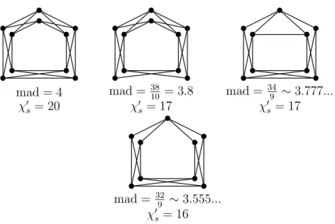
Figure

Documents relatifs
We show an upper bound for the maximum vertex degree of any z-oblique graph imbedded into a given surface.. Moreover, an upper bound for the maximum face degree
† Supported by the Ministry of Science and Technology of Spain, and the European Regional Development Fund (ERDF) under project-BFM-2002-00412 and by the Catalan Research Council
[1] proved that asymptotically every graph with maximum degree ∆ is acyclically colorable with O(∆ 4/3 ) colors; moreover they exhib- ited graphs with maximum degree ∆ with
If P does not end with v, then we can exchange the colors α and γ on this path leading to a δ-improper edge coloring such that the color γ is missing in u and v.. The color γ could
Rizzi, Approximating the maximum 3-edge-colorable subgraph problem, Discrete Mathematics 309
Proof Otherwise, we exchange colours along C in order to put the colour δ on the corresponding edge and, by Lemma 2, this is impossible in a
We consider the δ-minimum edge-colouring φ such that the edges of all cycles of F are alternatively coloured α and β except for exactly one edge per cycle which is coloured with δ,
In particular, strong chromatic indices of d-dimensional grids and of some toroidal grids are given along with approximate results on the strong chromatic index of
