HAL Id: hal-01007279
https://hal.archives-ouvertes.fr/hal-01007279
Submitted on 11 Feb 2017
HAL is a multi-disciplinary open access
archive for the deposit and dissemination of
sci-entific research documents, whether they are
pub-lished or not. The documents may come from
teaching and research institutions in France or
abroad, or from public or private research centers.
L’archive ouverte pluridisciplinaire HAL, est
destinée au dépôt et à la diffusion de documents
scientifiques de niveau recherche, publiés ou non,
émanant des établissements d’enseignement et de
recherche français ou étrangers, des laboratoires
publics ou privés.
Distributed under a Creative Commons Attribution| 4.0 International License
Sensitivity approach for modeling Stochastic Field of
Keulegan-Carpenter and Reynolds numbers through a
matrix response surface
Franck Schoefs, Morgan Boukinda
To cite this version:
Franck Schoefs, Morgan Boukinda. Sensitivity approach for modeling Stochastic Field of
Keulegan-Carpenter and Reynolds numbers through a matrix response surface. Journal of Offshore Mechanics
and Arctic Engineering, American Society of Mechanical Engineers, 2009, 132 (1), �10.1115/1.3160386�.
�hal-01007279�
Franck
Schoefs
Morgan L. Boukinda
Institute in Civil and Mechanical Engineering (GeM), Nantes Atlantic University, CNRS UMR 6183, 2 rue de la Houssinière, 44072 Nantes Cedex 03, France
Sensitivity Approach for Modeling Stochastic Field of
Keulegan–Carpenter and Reynolds Numbers Through
a Matrix Response Surface
The actual challenge for requalification of existing offshore structures through a rational process of reassessment indicates the importance of employing a response surface meth-odology. At different steps in the quantitative analysis, quite a lot of approximations are performed as a surrogate for the original model in subsequent uncertainty and sensitivity studies. This paper proposes to employ a geometrical description of the nth order Stokes model in the form of a random linear combination of deterministic vectors. These vectors are obtained by rotation transformations of the wave directional vector. This facilitates introduction of an appropriate level of complexity in stochastic modeling of the wave velocity and of the Reynolds and Keulegan–Carpenter numbers for probabilistic mechan-ics analysis of offshore structures. In situ measurements are used to assess suitable ranges and distributions of basic variables.
Keywords: offshore structures, response surfaces, hydraulic parameters, Morison equations, wave loading
1 Introduction
Nowadays one-third of the existing offshore platforms require a life extension. It is well recognized that the application of proba-bilistic approaches gives an efficient quantitative means for updat-ing information and for measurupdat-ing the relative change in safety level compared with a predefined requirement. During the past 2 decades, the efforts were concentrated to develop methods and corresponding software for structural reliability analyses. Increas-ingly in practice, failure probabilities and/or reliability indices are introduced for elaboration of load and resistance factor design
共LRFD兲 rules 关1兴 and comparison of design proposals. The actual
challenge is to provide rational procedures and decision aid tools related to the requalification of offshore structures where the structural and mechanical integrities are important criteria.
The required structural behavior can be considered as the out-put of a system, which varies in response to the changing levels of several input variables. The response surface methodology共RSM兲 comes, of course, as a basic formal aid-tool关2,3,20兴. The response curves must be based on some prescribed understanding of the underlying mechanism关4兴. In particular, the time evolution of the wave propagation is usually described by second order partial differential equations within more or less simplified boundary and initial conditions, known as the Navier–Stokes equations. Useful reviews of wave loads acting on offshore structures are available in a series of articles 关5,6兴, which focuses on the deterministic aspects mainly.
Here it is proposed to develop a formal representation of the wave kinematics field following a geometrical viewpoint. The nth order Stokes model has the form of a sum of n vectors, each of
them being obtained through suitable homothety and rotation transformations of the wave direction vector. The homothety ra-tios and the rotation angles are random functions for which the stochastic fluctuations depend on the wave height and on the wave kinematics intensity process. Analyzing the structure for the rel-evant stochastic processes leads to the derivation of a response surface for Reynolds and Keulegan–Carpenter numbers suitable for fatigue and extreme loading computation in the presence of marine growth关7兴.
2 Geometrical Modeling of the Wave Kinematics and Building of Matrix Response Surface
Physical time scales of wave actions are taken into account with practical efficiency by identifying sea-states as stationary compo-nents of a piecewise second order stationary ergodic and differen-tiable mean square random process 关8兴. As an extension of the generalized harmonic analysis, the stochastic process theory con-siders functions indexed by space/time parameters and with values in a so called complete probability space关9兴. One way of describ-ing a stochastic process is to specify the n-dimensional joint prob-ability law whatever n. Another means is to give an explicit for-mula for the value of the process at each index point in terms of a family of random variables whose probability law is known共e.g., trajectories兲. The last option is retained to describe wave by wave particle velocities on jacket platforms.
There is no magic guidance to generate such formulas by se-lecting among mathematical models 共e.g., Stokes, Boussinesq, Miche, etc.兲 for an application to ocean wave actions. Physical reasoning and observations give some classifications based on de-terministic criteria. But these theoretical models have to be intro-duced in a reliability analysis, regarding their stochastic nature due to their sensitiveness to random or uncertain parameters. This drives the safety domain topology and its probability measure. To this extent a formal geometrical representation of the wave kine-matics within a special care on Stokes waves is proposed.
2.1 Matrix Response Surface of Airy Wave. Let
共O,OX,OY,OZ兲 be an orthonormal basis in the Euclidean space
R3. The origin O is taken at the mean sea level, the axis OZ is vertical and upward, and OX is the wave directional axis. The following set of time and dimensionless in space indices is con-sidered: t, x = X/l, and z=Z/d+1, where l is the width of the structure共diameter of a cylinder containing the platform兲 and d is water depth. The small amplitude plane harmonic progressive waves known as airy waves are the simplest of all solutions to the wave problem. They are derived from a velocity potential also called orthogonal stream function. The associated velocity vector
VAiry takes the classical form 共see Eq. 共1兲兲 in the wave plane
共OX,OZ兲 VAiry= H 2
冑
g d cosh共kdz兲 cosh共kd兲冑
kd tanh共kd兲冋
cos共klx −t兲 tanh共kdz兲sin共klx −t兲册
共1兲where H is the wave height, k is the wave number, is the
共angular兲 frequency, and t=t− 共 is the phase angle兲. The variables k and are linked together by the one to one dispersive relation共2= gk tanh共kd兲兲.
Equation共1兲 writes
VAiry=1共cos共␣1兲OX + sin共␣1兲OZ兲 共2兲 with
tan共␣1兲 =
具VAiry,OZ典
具VAiry,OX典= tanh共kdz兲tan共klx −t兲 共3兲
1=储VAiry储 = H 2
冑
g d cosh共kdz兲 cosh共kd兲冑
kd tanh共kd兲冑
1 − sin2共klx −t兲 cosh2共kdz兲 共4兲The velocity vector being in the wave plane, it can be written as a combination of a homothetyH and a rotation R, applied on the vector OX, in the geometrical form
VAiry=H共O,1兲oR共− OY,␣1兲OX 共5兲 whereH共O,1兲 denotes the homothety with center O and ratio 1 and R共−OY,␣1兲 denotes the rotation of 共−OY兲 axis 共with −OV = OX∧OZ兲 and with angle␣1.
Expression共5兲 allows analyzing the kinematics field 共here ve-locity兲 by separating the intensity and the angle of the vector. The homothety ratio 1 and rotation angle␣1 are random functions indexed by共x,z,t兲. The fluctuations of their trajectories are de-pending on the couple of random variables 共H,k兲. Angle ␣1 is analytically independent of variable H.
The range and statistics of k are well adapted to approximate the vector W = R共−OY,␣1兲OX by the normalized first order Taylor expansion W共1兲around the mean wave number k¯. Subsequently some algebraic operations and differentiations are obtained as fol-lows:
W共1兲= W共k¯兲 + 共k − k¯兲W⬘共k兲兩k=k¯ where
W共k¯兲 = R共− OY,␣1兲OX with ␣1=␣1共k¯兲, 1=共k − k¯兲
␣ k共k¯兲 W⬘共k兲兩k=k¯=␣1⬘R
冉
− OY, 2冊
Wជ 共k¯兲 =␣1⬘R共− OY,␣1兲 ⴰ R冉
− OY, 2冊
OX 共6兲 Finally, W共1兲writes W共1兲=H冉
O,冑
1 1 +1 2冊
⫻o
再
Id +H共O,1兲oR冉
− OY,
2
冊
冎
oR共− OY,␣1兲OX共7兲
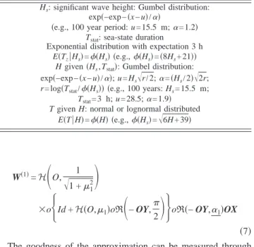
The goodness of the approximation can be measured through the scalar product of the two vectors共see Eq. 共8兲兲. It is given by considering in the wave plane the distance between the point N of the unit circle and with coordinates共cos共␣1−␣1兲;sin共␣1−␣1兲兲 and the straight line共D兲 of equation 共X+1Z = 0兲. Coordinates of N and direction of D vary with k. The Latin hypercube sampling technique is implemented to generate preliminary samples from the joint probability distribution for共H,k兲 of the extreme sea-state referenced in Table 1. Figure 1 presents a simulation of this dis-tance and statistics of k around k¯; s denotes the standard deviation. It is shown that whatever the statistics, the perpendiculars to D contain all the point O, origin of the repair and the approximation can be considered as very accurate.
cos共兲 = 具W共1兲,W典 =cos共␣1−␣គ1兲 +1sin共␣1−␣គ1兲
冑
1 +12 共8兲
Introducing inside Eq.共5兲 the approximation W共1兲instead of W, the velocity field corresponding has the following response curve:
Table 1 Extreme sea state parameters†10‡
Hs: significant wave height: Gumbel distribution:
exp共−exp−共x−u兲/␣兲
共e.g., 100 year period: u=15.5 m;␣= 1.2兲
Tstat: sea-state duration
Exponential distribution with expectation 3 h
E共Tz兩Hs兲=共Hs兲 共e.g.,共Hs兲=共8Hs+ 21兲兲
H given共Hs, Tstat兲: Gumbel distribution:
exp共−exp−共x−u兲/␣兲; u=Hs
冑r
/2;␣=共Hs/2兲冑
2r;r = log共Tstat/共Hs兲兲 共e.g., 100 years: Hs= 15.5 m;
Tstat= 3 h; u = 28.5;␣= 1.9兲 T given H: normal or lognormal distributed
E共T兩H兲=共H兲 共e.g.,共Hs兲=
冑
6H + 39兲VAiry⬇ VAiry共1兲 = a1A + b1B 共9兲 where A and B are deterministic orthonormal vectors defined by
A = R共− OY,␣1兲OX and B = R
冉
− OY,
2
冊
A and the coefficients a1and b1are random functionsa1=
1
冑
1 +12, b1=1a1
The random variable1is zero-mean and with narrow support. It follows that b1 is small compared with a1. Consequently A represents the main axis for the velocity vector and the component following B gives the fluctuations of the velocity vector inside a narrow sector around A.
2.2 Analysis of Stochastic Structure of Airy Wave Velocity.
The previous matrix response surface format of the velocity field for airy waves allows investigation of the stochastic structure of this stochastic field through its trajectories.
2.2.1 Role of Phase Angle . The pseudophase t play a particular role on variability of fields defined previously. It con-tains a time index t, a hazard introduced by共angular兲 frequency, and a phase which defined the position of the wave on the struc-ture. In fact,tbeing only in sine and cosine functions, its influ-ence can be seen as a change in repair by translation along the wave propagation axis whose origin varies with 共angular兲 fre-quency. In the following, it is assumed thatt= 0共e.g., initial time and the wave crest is on the first pile of the structure兲.
2.2.2 Study of Stochastic Field 1, Wave Velocity Intensity. The intensity of the velocity vector VAiryequals1. Equation共4兲 indicates that the scalar velocity intensity can be factorized
1= H 2
冑
g d cosh共kdz兲 cosh共kd兲冑
kd tanh共kd兲D共k,x,z,t兲 共10兲 where D共k,x,z,t兲 =冑
1 −sin 2共klx − t兲 cosh2共kdz兲is a function of the random variable k. This function varies slowly when k varies on its support and is the only function indexed by t and x. In order to illustrate this stochastic property, let us consider the extreme sea-state referenced in Table 1. Figure 2 presents the variation of D versus x at a depth z = 0.8共Z=−20 m兲 obtained for
the five statistics of k: mean value k¯, mean value plus/minus stan-dard deviation, and mean value plus/minus two times stanstan-dard deviation. The coefficient of variation does not exceed 1% at this depth, which is in the wave area. Denoted by Dគ , the value of D for k = k¯, Eq. 共10兲 is then transformed into a deterministic linear rela-tionship共11兲 between two random fields
1共x,z,t兲 = Dគ共x,z,0兲1共1兲共z兲 共11兲 This property is of course very interesting when investigating the stochastic properties of the wave velocity intensity. Let M = aN共a⫽0兲 be a linear relation between two random variables. It is well known that their densities are related by fM共n兲 = 1/a fN共n/a兲. In particular the density fMbecomes tighter when
兩a兩⬍1.
Function D is by definition upper-bounded by 1 and in the wave area, it can be shown that the term cosh共kdz兲 becomes dominant in comparison to sin共klx兲. D remains in fact very close to 1 and density distributions of1will be tightening only for the highest values of x in comparison to1共1兲. Suppose now thatt⫽0, the assertions remain true once extended the deterministic factor to Dគ 共x,z,t兲 by fixingtat the corresponding value to the mean wave number.
As the random velocity function1共1兲is indexed by z only, it is deduced that the coefficient of variation and the normalized sta-tistical moments of1 共skewness, kurtosis, etc.兲 vary only with this profile index z. As a consequence, the intensity of the airy wave is a profile random function for normalized statistics.
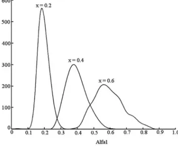
2.2.3 Study of the Orientation␣1of Velocity Vector. When1 represents the intensity of the wave velocity vector, angle␣1gives the main direction of this vector. It is noted that tanh共kdz兲 varies slowly with k and may be concentrated at its value for k = k¯. As an illustration and for variables previously presented in Table 1, Fig. 3 plots this function varying with x for the same five statistics of k: it is very close to tanh共k¯dz兲 whatever k. For given values of x, the distributions of␣1obtained from this relationship at depth 0.8 and varying with z are presented, respectively, in Figs. 4 and 5.
Then tan共␣1兲 behaves as a deterministic linear transformation of tan共klx−t兲. Equation 共3兲 can be expressed as a linear relation between two random fields
tan共␣1兲 = tan共klx − t兲 with  = tanh共k¯dz兲 共12兲 As a consequence the coefficients of variation and the normal-ized moments of ␣1共x,z,t兲 are depending of the indices x and t
only. They are constant whatever the index z. Moreover, in the vicinity of the mean sea level, coefficient is very close to 1. In this condition the angle␣1is well approximated as klx −t.
2.2.4 Study of Stochastic Field1. From Eq.共9兲, the stochas-tic field1is defined as the projection of the wave velocity vector on the deterministic vector B. The stochastic analysis of 1 is easier because this field is proportional to共k−k¯兲. This stochastic field is then centered and with a similar distribution to k after linear transformation. Consequently, fluctuations of1are weak and its spatial variability is directly linked to the one of␣1
⬘
共Eq.共13兲兲:
␣1⬘= lx tanh共k¯dz兲
1 + tan2共k¯lx兲
1 + tan2共k¯dz兲tan2共k¯lx兲 共13兲 In particular in the vicinity of the mean sea level共wave area兲, the approximation␣1
⬘
= lx is viable. It demonstrates that1is in-dependent of the index z. For the study of time dependency, pre-vious results are extended to the caset⫽0,␣1⬘=
冉
lx − k共k¯兲t冊
tanh共k¯dz兲 1 + tan2共k¯lx −t + 兲 1 + tanh2共k¯dz兲tan2共k¯lx −t + 兲 共14兲In the vicinity of the mean sea level, Eq.共14兲 becomes
␣1⬘=
冉
lx − k共k¯兲t
冊
In this condition the stochastic field1is linearly time depen-dent.
2.3 Expansion to the Matrix Response Surface of the nth Order Stokes Model. The nth order potential being the sum of a
set of n potentials, the response surface of each term i is obtained by a similar transformation based on a Taylor expansion of each term共see Eq. 共7兲兲.
Vi= aiAi+ biBi 共15兲 where Aiand Biare two deterministic orthogonal vectors in the wave plane:
Ai= R共− OY,␣i兲OX, Bi= R
冉
− OY,
2
冊
Ai ai=冑
i1 +i
2, bi=iai
After projection of these vectors on A and B, the response surface of nth order wave velocity is deduced共Eq. 共16兲兲
Vn= anA + bnB 共16兲 The multipliers anand bnare analytical random functions
an=
兺
i=1 n共aicos⌬i− bisin⌬i兲
bn=
兺
i=1 n共aisin⌬i+ bicos⌬i兲 where ⌬i=␣i−␣1 共17兲 They are expressed as functions of the wave height and of the wave period. Thus their stochastic fluctuations are governed by the randomness of these basic variables. The complexity level is discussed when order共n兲 is selected in the random functions a共n兲 and b共n兲. Note that each angle is deduced from relationship共18兲. tan共␣i兲 = tanh共ikdz兲tan关i共klx −t兲兴 共18兲 By implementing previous reasoning for each order, we may conclude that in the vicinity of the mean sea level, ␣i is well approximated to i共klz−t兲 and thus to i␣1. This approximation remains with depth where angles are weaker. In fact a larger rela-tive difference may be accepted for smaller mean values. Then the approximation␣i⬇i␣1may be assumed and the⌬iin Eq.共17兲 is well approximated by共i−1兲␣1. Equation共17兲 makes the sensitiv-ity analysis easier since each term of order共n兲 can be expressed as an additional perturbation of the previous order共n−1兲.
3 Matrix Response Surface of Reynolds and
Keulegan–Carpenter Numbers
3.1 General Formulation of Response Surfaces for Re and KC. For engineering purposes, it is now well admitted that
Mori-son equations give the main trends for the computation of hydrau-lic forces关11兴. The set of coefficients 共CD, CM, CX, and CX
⬘
兲 of the Morison equations depend on the hydraulic numbers: the Rey-nolds Re and the Keulegan–Carpenter KC numbers共Eqs. 共17兲 and共18兲兲 关12–15兴. The American Petroleum Institute code 关16兴 and
the future ISO regulations adopt the corresponding nonlinear
re-Fig. 4 Probability density of␣1„x , 0.8…for three values of x
lationships 共ISO/DIS 19902, 2004兲. Rather than these numbers, Stokes parameter or Strouhal number can be used.
Re =maxt苸关0;T/2兴共V⬜ 共n兲共t兲兲D 共19兲 KC =maxt苸关0;T/2兴共V⬜ 共n兲共t兲兲T D 共20兲
where V⬜共n兲共t兲 is the intensity 共in m/s兲 of the projection of the particle velocity onto the plane orthogonal to the beam, D is the diameter of the beam共m兲, T the wave period 共s兲, and is the kinematics viscosity of sea water 共m2/s兲. Here the velocity is computed from the Stokes model of order n.
As a consequence, Re and KC are random fields indexed by z. The field of particle velocity being expressed in the plane
共O,OX,OZ兲 in global repair, local coordinates 共Ob, xb, yb, and zb兲 are defined for its projection where xbis oriented by the beam axis and共yb, zb兲 is the plane orthogonal to the beam. By denoting 兿b, the orthogonal projection onto the beam axis and兿b⬜ the projec-tion onto the orthogonal plane to the beam, we obtain the response surfaces of Re and KC in Eqs.共21兲 and 共22兲.
Re = maxt苸关0;T/2兴
共
储
兿
b ⬜ 共a共t兲共n兲A共t兲 + b共t兲共n兲B共t兲兲储
兲
D 共21兲 KC = maxt苸关0;T/2兴共
储
兿
b⬜ 共a共t兲共n兲A共t兲 + b共t兲共n兲B共t兲兲储
兲
T D 共22兲In case of vertical component and by using Eq. 共16兲, these equations become Eqs.共23兲 and 共24兲.
Re =maxt苸关0;T/2兴共储a共t兲共n兲cos共␣1兲 − b共t兲共n兲sin共␣1兲储兲D
共23兲
KC =maxt苸关0;T/2兴共储a共t兲共n兲cos共␣1兲 − b共t兲共n兲sin共␣1兲储兲T
D 共24兲
In case of horizontal component, they become Eqs. 共25兲 and
共26兲.
Re =maxt苸关0;T/2兴共储a共t兲共n兲sin共␣1兲 − b共t兲共n兲cos共␣1兲储兲D
共25兲
KC =maxt苸关0;T/2兴共储a共t兲共n兲sin共␣1兲 − b共t兲共n兲cos共␣1兲储兲T
D 共26兲
Note that in practice, support of distribution for H and T are truncated in view to represent only physical events, then maxi-mum values can be determined.
3.2 Response Surfaces in Cases of Marine Growth Presence. In cases of marine growth presence, D must be replaced
in Eqs. 共19兲–共26兲 by mg D where mg is a multiplying factor. Generally, it is modeled by a random field indexed by z关17兴. 4 Numerical Studies
Consider the field of extreme waves presented in Table 1. Re-sponse surfaces of Re and KC are considered. It is suggested to analyze these stochastic fields indexed by z both through the evo-lution of statistics with depth and through the distributions at given depth. Modified Latin hypercube sampling technique is used for simulations关18兴. It allows reducing the size of samples
共here 1500兲. Convergence tests show that the relative error on
variance is about 5% in this case.
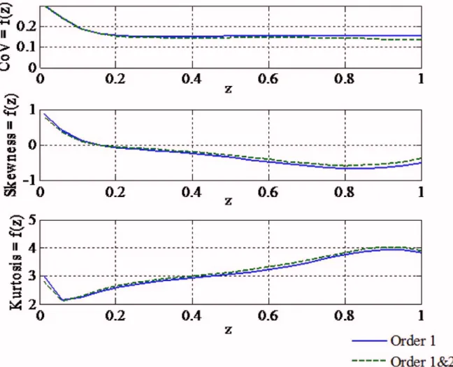
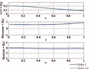
Figures 6 and 7 present the evolution of the coefficient of varia-tion, the skewness, and the kurtosis with depth for a vertical com-ponent of diameter 1 m. These statistical moments give the main information on the shape of the distribution. Only the first and the second order of the Stokes model are plotted.
First, when considering the order of the Stokes model, it is shown that the first order is sufficient to predict the main trends of the evolution with depth. It is noticed that the evolution of these statistics with depth is strong and that the coefficients of variation
near the splash area共z=1兲 are, respectively, of 15% for Re and 9% for KC. Note that except at the bottom, the coefficient of variation of Re remains constant value with depth. As the mean value is strongly decreasing with depth, the variance is decreasing too. The symmetry of Re共see sign of skewness兲 can change with depth. This property is of significant importance for reliability studies and is underlined with Figs. 8 and 9 where distributions of Re, respectively, at depth 50 m 共z=0.5兲 and 100 m 共z=0兲 are given.
5 Conclusions
This paper suggests a new matrix response surface for stochas-tic modeling of Reynolds and Keulegan–Carpenter numbers. It starts from a geometrical modeling of the wave kinematics field based on the Stokes model. The stochastic properties of the geo-metrical parameters are analyzed and a complete expansion is provided. It takes the form of a summation of stochastic coeffi-cients, with known properties, with space, acting on deterministic vectors. Items such as physical meanings, complexity level in modeling, distribution effects, and computational tractability are addressed. They are essential criteria for an operational use of RSM in a reliability analysis. It allows discussing the complexity level to introduce in the Stokes model. Results are site specific and an illustration is given on a site in the North Sea关19,20兴. This new approach provides an algorithmic improvement of the com-puter module on wave loading, which is available in different packages such as the evaluation of jackets from a probabilistic redundant analysis共ARPEJ兲 and the reliability analysis system for
offshore structures共RASOS兲.
References
关1兴 Joint Committee on Structural Safety, 2001, “Probabilistic Model Code,”
JCSS Paper No. JCSS-OSTL/DIA/VROU-10-11-2000, www.jcss.ethz.ch.
关2兴 Labeyrie, J., 1990, Stochastic Load Models for Marine Structure Reliability,
3rd ed., IFIP WG, Berkley, CA.
关3兴 Schoefs, F., Le Van, A., and Rguig, M., 2008, “Cracked Finite Element for
Through-Cracked Tube,” Commun. Numer. Methods Eng., 24, pp. 761–775.
关4兴 Labeyrie, J., and Schoefs, F., 1995, “A Discussion on Response Surface
Ap-proximations for Use in Structural Reliability,” Reliability and Optimization of Structural Systems, Chapman and Hall, Assisi, Italy, pp. 161–168.
关5兴 Lightill, J., 1986, “Fundamentals Concerning Wave Loadings on Offshore
Structures,” J. Fluid Mech., 173, pp. 667–681.
关6兴 Standing, R. G., 1984, “Wave Loading on Offshore Structures, A Review,”
Ocean Science and Engineering, 9, pp. 25–134.
关7兴 Schoefs, F., Boukinda, M., Birades, M., Lahaille, A., and Garretta, R., 2004,
“Modeling of Marine Growth Effect on Offshore Structures Loading Using Kinematics Field of Water Particle,” Proceedings of the 14th International Offshore and Polar Engineering Conference共ISOPE兲, Toulon, France, pp.
Fig. 7 First statistics of KC as function of z for a vertical beam
Fig. 9 Distribution of Re for a vertical beam„Z = −100 m…
419–426.
关8兴 Labeyrie, J., 1990, “Stationary and Transient States of Random Seas,” Mar.
Struct., 3, pp. 43–58.
关9兴 Parzen, E., 1967, Stochastic Process, Holden-Day, San Francisco, CA. 关10兴 Doucet, Y., Labeyrie, J., and Thebault, J., 1987, “Validation of Stochastic
Environmental Design Criteria in the Frigg Field,” Adv. Underwater Technol. Ocean Sci. Offshore Eng., 12, pp. 45–59.
关11兴 Morison, J. R., O’Brien, M. P., Johnson, J. W., and Schaff, S. A., 1950, “The
Force Exerted by Surfaces Waves on Piles,” Journal of Petroleum Technology, AIME, 189, pp. 149–154.
关12兴 Sarpkaya, T., 1976, “In-line and Transverse Forces on Smooth and Sand
Roughened Circular Cylinders in Oscillating Flow at High Reynolds Num-bers,” Technical Report No. NPS-69SL-76062.
关13兴 Sarpkaya, T., 1990, “On the Effect of Roughness on Cylinders,” ASME J.
Offshore Mech. Arct. Eng., 112, pp. 334–340.
关14兴 Theophanatos, A., 1988, “Marine Growth and Hydrodynamic Loading of
Off-shore Structures,” Ph.D. thesis, University of Strathclyde, Strathclyde, UK.
关15兴 Wolfram, J., Jusoh, I., and Sell, D., 1993, “Uncertainty in the Estimation of the
Fluid Loading Due to the Effects of Marine Growth,” ASME J. Offshore Mech. Arct. Eng., 2, pp. 219–228.
关16兴 American Petroleum Institute, 2004, “Recommended Practice for Planning,
Designing and Constructing Fixed Offshore Platforms—Working Stress De-sign,” API Report No. RP2A-WSD.
关17兴 Boukinda Mbadinga, M., Schoefs, F., Quiniou, V., and Birades, M., 2007,
“Marine Growth Colonization Process in Guinea Gulf: Data Analysis,” ASME J. Offshore Mech. Arct. Eng., 129共2兲, pp. 97–106.
关18兴 Iman, R. L., Helton, J. C., and Campbell, J. E., 1981, “An Approach to
Sen-sitivity Analysis of Computer Models—Part I: Introduction, Input Variable Selection and Preliminary Variable Assessment,” J. Quality Technol., 13共3兲, pp. 174–183.
关19兴 Schoefs, F., 1996, “Response Surface of Wave Loading for Reliability of
Ma-rine Structures,” Ph.D. thesis, University of Nantes, Nantes, France.
关20兴 Schoefs, F., 2008, “Sensitivity Approach for Modelling the Environmental
Loading of Marine Structures Through a Matrix Response Surface,” Reliab. Eng. Syst. Saf., 93共7兲, pp. 1004–1017.