How did Marine Isotope Stage 3 and Last Glacial Maximum climates differ? – Perspectives from equilibrium simulations

HAL Id: hal-03199345

https://hal.archives-ouvertes.fr/hal-03199345

Submitted on 15 Apr 2021

HAL is a multi-disciplinary open access

archive for the deposit and dissemination of

sci-entific research documents, whether they are

pub-lished or not. The documents may come from

teaching and research institutions in France or

abroad, or from public or private research centers.

L’archive ouverte pluridisciplinaire HAL, est

destinée au dépôt et à la diffusion de documents

scientifiques de niveau recherche, publiés ou non,

émanant des établissements d’enseignement et de

recherche français ou étrangers, des laboratoires

publics ou privés.

Maximum climates differ? – Perspectives from

equilibrium simulations

C. van Meerbeeck, H. Renssen, Didier M. Roche

To cite this version:

C. van Meerbeeck, H. Renssen, Didier M. Roche. How did Marine Isotope Stage 3 and Last Glacial

Maximum climates differ? – Perspectives from equilibrium simulations. Climate of the Past, European

Geosciences Union (EGU), 2009, 5 (1), pp.33-51. �10.5194/cp-5-33-2009�. �hal-03199345�

www.clim-past.net/5/33/2009/

© Author(s) 2009. This work is distributed under the Creative Commons Attribution 3.0 License.

Climate

of the Past

How did Marine Isotope Stage 3 and Last Glacial Maximum

climates differ? – Perspectives from equilibrium simulations

C. J. Van Meerbeeck1, H. Renssen1, and D. M. Roche1,2

1_{Department of Earth Sciences - Section Climate Change and Landscape Dynamics, Faculty of Earth and Life Sciences, VU} University Amsterdam, de Boelelaan 1085, 1081HV Amsterdam, The Netherlands

2_{Laboratoire des Sciences du Climat et de l’Environnement (LSCE/IPSL), Laboratoire CEA/INSU-CNRS/UVSQ, C.E. de} Saclay, Orme des Merisiers Bat. 701, 91190 Gif sur Yvette Cedex, France

Received: 15 August 2008 – Published in Clim. Past Discuss.: 6 October 2008 Revised: 14 January 2009 – Accepted: 20 February 2009 – Published: 5 March 2009

Abstract. Dansgaard-Oeschger events occurred frequently during Marine Isotope Stage 3 (MIS3), as opposed to the fol-lowing MIS2 period, which included the Last Glacial Max-imum (LGM). Transient climate model simulations suggest that these abrupt warming events in Greenland and the North Atlantic region are associated with a resumption of the Ther-mohaline Circulation (THC) from a weak state during sta-dials to a relatively strong state during interstasta-dials. How-ever, those models were run with LGM, rather than MIS3 boundary conditions. To quantify the influence of different boundary conditions on the climates of MIS3 and LGM, we perform two equilibrium climate simulations with the three-dimensional earth system model LOVECLIM, one for sta-dial, the other for interstadial conditions. We compare them to the LGM state simulated with the same model. Both cli-mate states are globally 2◦C warmer than LGM. A striking feature of our MIS3 simulations is the enhanced Northern Hemisphere seasonality, July surface air temperatures being 4◦C warmer than in LGM. Also, despite some modification in the location of North Atlantic deep water formation, deep water export to the South Atlantic remains unaffected. To study specifically the effect of orbital forcing, we perform two additional sensitivity experiments spun up from our sta-dial simulation. The insolation difference between MIS3 and LGM causes half of the 30–60◦N July temperature anomaly (+6◦_{C). In a third simulation additional freshwater forcing}

halts the Atlantic THC, yielding a much colder North At-lantic region (−7◦_{C). Comparing our simulation with proxy}

data, we find that the MIS3 climate with collapsed THC

Correspondence to:

C. J. Van Meerbeeck

(cedric.van.meerbeeck@falw.vu.nl)

mimics stadials over the North Atlantic better than both con-trol experiments, which might crudely estimate interstadial climate. These results suggest that freshwater forcing is nec-essary to return climate from warm interstadials to cold sta-dials during MIS3. This changes our perspective, making the stadial climate a perturbed climate state rather than a typical, near-equilibrium MIS3 climate.

1 Introduction

Marine Isotope Stage 3 (MIS 3) – a period between 60 and 27 ka ago during the last glacial cycle – experienced sev-eral abrupt climatic warming phases known as Dansgaard-Oeschger (DO) events. Registered in Greenland ice core oxygen isotope records (see Fig. 1), DO events are abrupt transitions from cold, stadial climate conditions to mild, in-terstadial conditions, eventually followed by a return to cold stadial conditions (Dansgaard et al., 1993). Temperature re-constructions of DO shifts in Greenland suggest a rapid mean annual surface air temperature rise of up to 15◦C in a few decades (Severinghaus et al., 1998; Huber et al., 2006). In addition, within certain stadials, massive ice surges from the Laurentide Ice Sheet flushed into the North Atlantic Ocean during so-called Heinrich events (Heinrich, 1988). These DO events and Heinrich events (HEs) are correlated with rapid climatic change in the circum-North Atlantic region (Bond et al., 1993; van Kreveld et al., 2000; Hemming, 2004; Rasmussen and Thomsen, 2004). It is presently not clear, however, why DO events were so frequent during MIS 3, while being nearly absent around the Last Glacial Maximum (LGM). Here, the LGM is considered to be the period be-tween roughly 21 and 19 ka ago with largest ice sheets of the

-80 -60 -40 -20 0 20 40 60 80 70 60 50 40 30 10 0

Time (ka ago)

W m -2 -45 -43 -41 -39 -37 -35 -33 -31 -29 -27 -25 N G R IP δ 18O June-60N December-60N Jun-dec-amp-60N December-60S June-60S Dec-Jun-amp-60S

zero insolation anomaly NGRIPd18O

20 56k 32k 21k

_{MIS 3}

Insolation changes and NorthGRIP d18O curve for 70 ka BP to present

Figure 1 42

Fig. 1. The NorthGRIP18O curve (black – NorthGRIP Members, 2004) from 0 to 70 ka ago on the ss09sea time scale. MIS 3 is shaded in grey. Greenland interstadials DO 8, DO 12 and DO 14, and Heinrich events HE 4 and HE 5 are shown. Superimposed are the summer (dashed lines) and winter (dotted lines) insolation anomalies compared to present-day at 60◦N (dark blue) and 60◦S (light blue), which results from orbital changes. Our modelling ex-periments are setup with the orbital parameter values at 56, 32 and 21 ka BP, as marked in red. (Insolation is defined as the top-of-the-atmosphere incoming solar radiation).

last glacial. Therefore, we analyse in this paper some char-acteristic features of the MIS3 climate and compare them to the LGM climate, using climate modelling results.

Several attempts have been made to uncover the mecha-nisms that underlie millennial-scale glacial climatic changes. It has been hypothesised (e.g., Broecker et al., 1990) that DO events result from changes in strength of the Atlantic Thermohaline Circulation (THC). The onset of a DO event could represent a sudden resumption from a reduced or col-lapsed THC state during a stadial to a relatively strong in-terstadial state (Broecker et al., 1985). This would instan-taneously increase the northward oceanic heat transport in the Atlantic. The additional heat is then released to the at-mosphere in the mid- and high latitudes over and around the North Atlantic, mostly in winter time. The strength of At-lantic THC depends on the density of surface water masses in the high latitudes, where deep water can be formed through convection when the water column is poorly stratified. Strat-ification occurs when freshwater flows to convection sites in the high latitudes of the North Atlantic Ocean or the Nordic Seas. This could for instance have occurred during HEs, when the freshwater released by huge amounts of melting icebergs is thought to have caused a THC shutdown (e.g., Broecker, 1994; Stocker and Broecker, 1994).

It is currently uncertain what drives changes in ice sheet mass balance associated with HEs and DO events (Clark et al., 2007). A negative mass balance can be achieved by re-duced snow accumulation, ice calving or by enhanced melt-ing, or a combination of these processes. Either internal

os-cillations in the dynamics of the climate system, or variations in an external energy source can increase ablation. In the first case, a periodical decay of the ice volume takes place. Ac-cording to MacAyeal (1993)’s binge/purge model, approxi-mately every 7000 years, ice berg armada’s from the Lau-rentide Ice Sheet (HEs) occurred after basal melt lubricated the bedrock of the Hudson Bay and Hudson Strait, which created an ice stream (purge phase). Basal melt occurred af-ter several thousands of years of slow ice accumulation, as basal ice temperature increased to attain melting point due to growing geothermal heat excess and pressure from the over-lying ice (binge or growth phase). In the second case, en-ergy input into the climate system oscillates at a frequency aligned with DO event recurrence, or at a lower or higher fre-quency – if the frefre-quency of the events is modulated by the forcing (Ganopolski and Rahmstorf, 2002; Rial and Yang, 2007). An example of external forcing with lower frequency than DO recurrence is insolation changes by orbital forcing (Berger, 1978; Berger and Loutre, 1991; Lee and Poulsen, 2008). In the mid and high latitudes of the Northern Hemi-sphere the amount of insolation is mostly controlled by the obliquity and precession signals. July insolation at 65◦N has been higher during MIS 3 than at LGM, with an aver-age 446 W m−2over the 60–30 ka BP interval compared to 418 W m−2at 21 ka BP, see Fig. 1. This provided a positive summer forcing to the climate system, so more energy may have been available for ice melting, which may have resulted in the smaller ice sheets observed during MIS 3 than during MIS 4 and MIS 2 (e.g. Svendsen et al., 2004; Helmens et al., 2007).

In an effort to better understand the processes that drove MIS 3 climate over Europe, the Stage 3 project (van An-del, 2002) involved several modelling exercises designed at reproducing as closely as possible the reconstructions from proxy climate archives (Barron and Pollard, 2002; Pollard and Barron, 2003; Alfano et al., 2003; van Huissteden et al., 2003). Barron and Pollard (2002) and Pollard and Bar-ron (2003) concluded that MIS 3 variations in orbital forcing, Scandinavian Ice Sheet size, and CO2concentrations could not explain the differences between a cold state and a milder state registered in the records. They attributed part of the range of air temperature differences between the milder and the cold state to colder North Atlantic and Nordic Seas sea surface temperatures and the associated extended southward distribution of sea ice in the stadial state. The remaining tem-perature differences might be attributed to physical processes that are unsolved by their model, e.g. oceanic circulation changes. The main limitation of Barron and Pollard (2002) and Pollard and Barron (2003) is the use of a GCM without an interactive oceanic model. This means that they forced their atmospheric model with estimated MIS 3 SSTs for a cold state and a milder state. Their experiments were thus not designed to explain the mechanisms behind the oceanic circulation changes seen in data between stadials and inter-stadials (e.g. Dokken and Jansen, 1999).

Compared to the work of Barron and Pollard (2002) and Pollard and Barron (2003), we investigate several additional, potential drivers of MIS 3 climate change. We estimate the climate sensitivity to CO2, CH4and N2O as well as atmo-spheric dust concentration changes between stadial and in-terstadial values when the oceanic circulation and the atmo-spheric circulation are coupled. In addition, we investigate how, compared to LGM, stronger Northern Hemisphere sum-mer insolation and smaller ice sheet size affected the MIS 3 climate. To do so, we simulate two quasi-equilibrium states with the LOVECLIM earth system model (Driess-chaert, 2005). These states are obtained by imposing typical, but constant MIS 3 boundary conditions as well as stadial (MIS3-sta) and interstadial (MIS3-int) greenhouse gas and dust forcings, respectively.

To quantify the Northern Hemisphere summer warming caused by insolation changes, we perform two additional ex-periments, with all forcings and boundary conditions equal to MIS3-sta, except for the orbital parameters, which we set at 21 ka and 32 ka BP, respectively. We also studied the sen-sitivity of the THC strength to freshwater forcing in the ‘sta-dial’ state (MIS3-HE), as numerous such studies have shown that THC-shifts could indeed be responsible for millennial-scale climate variability during the last glacial (e.g., storf, 1996; Sakai and Peltier, 1997; Ganopolski and Rahm-storf, 2001; Schulz, 2002; Wang and Mysak, 2006; Weber et al., 2007). It is not clear to what extent these previous results are applicable to the MIS3 climate, as their authors have used LGM as an analogue of stadials. Concomitantly, with our sensitivity experiments, we compare our findings to those of Barron and Pollard (2002) and Pollard and Bar-ron (2003) regarding the surface air temperature impact of orbital changes during MIS 3 and reduced SSTs from a warm to a cold state. Finally, we elaborate on how to better design modelling experiments that study DO-like behaviour of the climate system.

2 Methods

2.1 Model

We performed our simulations with the three-dimensional coupled earth system model of intermediate complexity LOVECLIM (Driesschaert, 2005). Its name refers to five dynamic components included (LOCH-VECODE-ECBilt-CLIO-AGISM). In this study, only three coupled compo-nents are used, namely ECBilt – the atmospheric component, CLIO – the ocean component, and VECODE – the vegetation module.

The atmospheric model ECBilt is a quasi-geostrophic, T21 horizontal resolution spectral model – corresponding to

∼5.6◦latitude ×∼5.6◦ longitude – with three vertical lev-els (Opsteegh et al., 1998). Its parameterisation scheme allows for fast computing and includes a linear longwave

radiation scheme. ECBilt contains a full hydrological cy-cle, including a simple bucket model for soil moisture over continents, and computes synoptic variability associ-ated with weather patterns. Precipitation falls in the form of snow with temperatures below 0◦C. CLIO is a primitive-equation three-dimensional, free-surface ocean general cir-culation model coupled to a thermodynamical and dynami-cal sea-ice model (Goosse and Fichefet, 1999). CLIO has a realistic bathymetry, a 3◦latitude×3◦ longitude horizontal resolution and 20 levels in the vertical. The free-surface of the ocean allows introduction of a real freshwater flux (Tart-inville et al., 2001). In order to bring precipitation amounts in ECBilt-CLIO closer to observations, a negative precipitation flux correction is applied over the Atlantic and Arctic Oceans to correct for excess precipitation. This flux is reintroduced in the North Pacific. The climate sensitivity of ECBilt to a doubling in atmospheric CO2concentration is 1.8◦C, asso-ciated with a global radiative forcing of 3.8 W m−2 (Driess-chaert, 2005). The dynamic terrestrial vegetation model VE-CODE computes herbaceous plant and tree plus desert frac-tions in each land grid cell (Brovkin et al., 1997) and is cou-pled to ECBilt through the surface albedo.

LOVECLIM produces a generally realistic modern cli-mate (Driesschaert, 2005) and an LGM clicli-mate generally consistent with data (Roche et al., 2007).

2.2 Experimental design

In order to simulate realistic features of the MIS 3 climate, the model was first setup with LGM boundary conditions and forcings, then spun-up to quasi-equilibrium state (Roche et al., 2007). These forcings (Table 1) include LGM at-mospheric CO2, CH4and N2O concentrations, LGM atmo-spheric dust content (after Claquin et al., 2003) and 21 ka BP insolation (Berger and Loutre, 1992). Other boundary con-ditions were modified. Bathymetry and land-sea mask were adapted to a sea level 120 m below present-day (Lambeck and Chappell, 2001), and the ice sheet extent and volume was taken from Peltier (2004)’s ICE-5G 21k, interpolated on the ECBilt grid.

To obtain the MIS3-sta and MIS3-int simulations, the model was subsequently set-up for MIS3 conditions. The difference in the experimental setup between MIS3-sta and MIS3-int was only due to greenhouse gas and dust forcing, since the insolation and icesheets were kept identical. In both experiments, insolation was set to its 56 ka BP values (Berger and Loutre, 1991). Ice sheet extent and topography for MIS 3 were worked out as a best guess – with consider-ation of controversial evidence on their configurconsider-ation. They were modified after the ICE-5G modelled ice sheet topog-raphy (Peltier, 2004) averaged over 60 to 30 ka BP (using interpretations from Svendsen et al., 2004; Ehlers and Gib-bard, 2004) and interpolated at ECBilt grid-scale (see Fig. 2). We used the LGM land-sea mask in all our MIS 3 simula-tions. Considering the small area that would be influenced by

Table 1. Boundary conditions for our experiments compared to the LGM experiment.

CO2 CH4 N2O dust factor orbital forcing fresh water ice sheets land-sea mask

(ppmv) (ppbv) (ppbv) (ka BP) (Sv) (ka BP) (ka BP)

LGM 185 350 200 1 21 0 21 21 MIS3-sta 200 450 220 0.8 56 0 MIS 3 21 MIS3-int 215 550 260 0.2 56 0 MIS 3 21 MIS3-sta-32k 200 450 220 0.8 32 0 MIS 3 21 MIS3-sta-21k 200 450 220 0.8 21 0 MIS 3 21 MIS3-HE 200 450 220 0.8 56 0.3 MIS 3 21 0 0.3 0.6 0.9 1.2 1.5 1.8 2.1 2.4 2.7 km

MIS 3 ice sheets

Figure 2 43

Fig. 2. Best estimate average MIS 3 ice sheet extent (thick black line) and additional topography compared to present-day ones (colour scale).

a relative higher sea-level compared to LGM, we assume that the impact of using an LGM land-sea mask in our MIS 3 ex-periments is minor. Moreover, sea level reconstructions are scarce and poorly resolved for MIS 3, with estimated sea lev-els of approximately between 60 and 90 m below present-day sea level (Chappell, 2002). However, in our model, main-taining the LGM land-sea mask implies that the Barents and Kara Seas were for the most part land mass. Therefore we set the albedo of these grid cells to a constant value of 0.8, which is the same as for ice sheets. On a local scale, we only expect a small energy balance bias in using continental ice as the heat flux between ocean, sea-ice and the atmosphere are discarded for these cells.

MIS3-sta (MIS3-int) was additionally forced with average MIS 3 stadial (interstadial) atmospheric GHG concentrations and top of the atmosphere albedo taking into account the effect of elevated atmospheric dust concentrations (see Ta-ble 1). The GHG concentrations we used in the setup of MIS3-sta and MIS3-int are based on typical concentrations found in the ice core records for stadials, respectively inter-stadials 8 and 14 (Inderm¨uhle, 2000; Fl¨uckiger et al., 2004).

We made a stack of all records during these intervals and se-lected the (rounded) mean value of the spline functions in the stadials, respectively interstadials as final GHG concen-trations. The very much simplified dust forcing was calcu-lated by multiplying the grid cell values of the LGM forcing map of Claquin et al. (2003), adapted in Roche et al. (2007) with an empirical dust factor corresponding to a best-guess of the average atmospheric dust-content (following the NGRIP

δ18O record - NorthGRIP Members, 2004) during an MIS 3 stadial or interstadial. The factor is inferred from an expo-nential transfer function of the NorthGRIP δ18O record (we derived Eqs. 1–3), which explains most of the anticorrelation between the NorthGRIP dust and δ18O records. The dust factors are based on findings of Mahowald et al. (1999) and Mahowald et al. (2006) that, on average, globally the atmo-spheric dust content was about five times lower during inter-stadials compared to full glacial conditions. In the Greenland ice core records, dust concentration peaks during stadials did at times attain LGM values. Applying this to our parameter-isation, would give a dust factor of 1 in such cases. How-ever, averaged over the duration of a stadial, the dust content seems slightly lower than 21 ka ago. Therefore, we opted for a stadial average of 0.8. The transfer function is:

for δ18O ≤ −43 per mil → dust factor=1 (1) for δ18O ≥ −39 per mil → dust factor=0 (2)

else dust factor=5−δ18O−4 43 ₍₃₎

Starting from the LGM state, we ran the model twice – with the respective MIS3-sta and MIS3-int forcings – for 7500 years to obtain two states in quasi-equilibrium with MIS 3 “stadial” and “interstadial” conditions respectively. We com-pare the last 100 years of the results of our simulation with the LGM climate simulations of Roche et al. (2007). For cer-tain variables, output on daily basis is analysed over an addi-tional 50-year interval in order to carefully assess seasonality in Europe.

Table 2. Comparison of MIS3 and LGM surface air temperatures (in◦C, values between brackets are 1 σ ).

Area Global Europe North Atlantic South Ocean

◦ E −180 to 180 −12 to 50 −60 to −12 −180 to 180 ◦_{N −90 to 90 30 to 72 30 to 72 −65 to −50} Year LGM 11.5 (0.1) 4.1 (0.5) 5.1 (0.4) −4.4 (0.2) MIS3-sta 13.2 (0.1) 8.8 (0.5) 8.1 (0.5) −1.6 (0.2) MIS3-sta vs LGM 1.7 4.7 3.0 2.8 MIS3-int 13.5 (0.1) 9.5 (0.5) 9.0 (0.3) −0.5 (0.2) MIS3-int vs sta 0.3 0.7 0.9 1.1 MIS3-HE 12.0 (0.1) 1.4 (0.6) 1.4 (0.5) −1.2 (0.3) MIS3-HE vs sta −1.2 −7.4 −6.9 0.4 January LGM 10.0 (0.3) −4.9 (1.7) 1.4 (1.1) 1.6 (0.2) MIS3-sta 11.0 (0.2) −1.7 (1.3) 4.4 (0.7) 3.7 (0.2) MIS3-sta vs LGM 1.0 3.2 3.5 1.9 MIS3-int 11.3 (0.2) −0.9 (1.0) 5.5 (0.4) 4.0 (0.2) MIS3-int vs sta 0.4 0.7 0.4 0.6 MIS3-HE 9.7 (0.2) −9.4 (1.5) −4.4 (1.5) 3.9 (0.2) MIS3-HE vs sta −1.3 −7.7 −8.8 0.2 July LGM 13.9 (0.1) 16.1 (0.5) 10.1 (0.3) −11.7 (0.5) MIS3-sta 16.4 (0.1) 22.8 (0.6) 12.9 (0.4) −7.7 (0.5) MIS3-sta vs LGM 2.5 6.7 2.8 4.0 MIS3-int 16.7 (0.1) 23.2 (0.5) 13.6 (0.3) −6.8 (0.5) MIS3-int vs sta 0.3 0.4 0.7 0.9 MIS3-HE 15.6 (0.1) 17.0 (0.7) 7.8 (0.3) −8.1 (0.6) MIS3-HE vs sta −0.8 −5.8 −5.1 −0.4

3 MIS3-sta and MIS3-int climates vs. LGM climate 3.1 Atmosphere

3.1.1 Temperature

Globally, our modelled MIS 3 climates are significantly warmer than LGM, especially during boreal summer (see Fig. 3 and Table 2). The global mean July surface air temper-ature (SAT) anomalies compared to LGM are +2.5±0.2◦C (±0.2 means 2σ =0.2) for MIS3-sta and +2.8±0.4◦C for MIS3-int. Moreover, the Northern Hemisphere (NH) fea-tures stronger warm anomalies than the Southern Hemi-sphere (SH) with NH July SAT anomalies of +3.5±0.4◦_C

for MIS3-sta and 3.8±0.4◦_{C for MIS3-int, whereas they are}

+0.9±0.4◦C and +1.1±0.4◦C respectively for the SH Jan-uary SAT anomalies. As can be seen from Fig. 3f, the differ-ences in SAT between MIS3-int and MIS3-sta are relatively small (mostly below 1◦C), and in many locations not signif-icant to the 99% confidence level. However, when upscaling to continental size or ocean basin size, some SAT differences are significant (see Table 2). We therefore compare

MIS3-sta with LGM and only discuss the MIS3-statistically significant differences between MIS3-sta and MIS3-int.

The high-latitude summers are vigorously warmer in MIS3-sta than in LGM, as is depicted in Fig. 3c. In the NH, the July SAT anomaly is +5◦C to more than +15◦C warmer in MIS3-sta. Regionally, the strongest warm anomalies are found in northern Russia, the Arctic Ocean (+5◦C to +15◦C, especially in September, not shown), the Nordic Seas, and Canada and Alaska. In the SH the warm anomalies are some-what attenuated, with January SAT anomalies of +3◦_{C to}

+10◦_{C over coastal Antarctica (see Fig. 3d). For that month,}

the Labrador Sea and parts of the Artic Ocean and Nordic Seas show the largest positive anomalies of up to +25◦C.

Some mid-latitudinal regions experience much warmer temperatures in MIS3-sta during summer as well (see Fig. 3c), with +3◦C to +10◦C and more in the NH. Over the NH mid-latitude oceans, however, the strongest warm anomaly is confined to +3.5◦C over the North Atlantic sec-tor. In comparison, in the SH, January and July anomalies of +1◦C to +5◦C occurred over Antarctica and the Southern Ocean respectively. Only weak, and in many areas not sig-nificant SAT differences are noted elsewhere in the SH mid

a) LGM July SAT b) LGM January SAT °C °C °C °C not sign.

c) MIS3-sta minus LGM July SAT anomaly d) MIS3-sta minus LGM January SAT anomaly

e) MIS3-sta minus MIS3-int July SAT anomaly f) MIS3-sta minus MIS3-int January SAT anomaly

g) LGM July minus January SAT range h) MIS3-sta minus LGM July minus January SAT range anomaly

Figure 3

Fig. 3. (a–f) July (left panels) and January (right panels) SATs for LGM (a and b), MIS3-sta minus LGM anomaly (c and d), MIS3-int minus

MIS3-sta anomaly (e and f); (g) LGM seasonal SAT range (July minus January); (h) Seasonal SAT range anomaly for MIS3-sta minus LGM.

latitudes (see Fig. 3d). Winters show contrasting response to the imposed forcings and boundary conditions in the mid latitudes. Whereas the entire western Eurasia, part of the North Atlantic and the mid latitude SH are warmer in Jan-uary in our MIS3-sta simulation than in LGM, no significant signal is registered in most other regions. Two exceptions are the United States east of the Rocky Mountains and Southern Siberia, which exhibit some cooler January SATs.

Further away from the poles, July SAT anomalies of +1◦_C

to as much as +5◦C in the NH continental subtropics are found. Arid and semi-arid regions of northern Africa and in central and western China experience the strongest positive signal. Over the oceans, warming is mostly limited to +1◦C (see Fig. 2c). Interestingly, January anomalies are negative over the Australian deserts, and some subtropical SH loca-tions as well as equatorial Africa. The remaining subtropical and all tropical regions, with the exception of certain patches over land, showed warming of less than +1◦C.

Subtracting the absolute values of the January from the July SATs, we obtain an approximation of the seasonal range and hence the continentality. As can be seen from Fig. 3g, in our LGM simulation, the range is usually smaller over the ocean than over the continent at any latitude, and in both cases becomes larger moving pole wards from the equator (less than 2◦C) to the high latitudes (from about 20◦C to as much as 70◦C). Over the continents, one may observe an increase towards the east in the mid latitudes. Over the ice sheets, the seasonal temperature range is usually reduced (to about 20◦_{C) compared to the latitudinal average. The}

anomaly of MIS3-sta minus LGM (Fig. 3h) shows a clearly larger seasonal range over much of the NH, especially in the high latitudes. Notable exceptions are the Labrador Sea and parts of the Nordic Seas – where the SAT seasonality range is strongly reduced. Over the SH, not much change is noted north of 55◦S, whereas relatively strong differences appear over the Southern Ocean and coastal Antarctica for our July– January approximation.

When comparing MIS3-int to MIS3-sta finally (Fig. 3e, f), the only regions showing significantly warmer winters and summers were located around Antarctica and above the Labrador and Nordic Seas, respectively over NW Canada, and to a lesser extent than in January also the Labrador Sea. Overall, as reflected by the global annual mean SATs, MIS3-int was slightly warmer than MIS3-sta by +0.4◦C, both in January and July (see Table 2).

3.1.2 Northern Hemisphere atmospheric circulation and global precipitation

In the NH mid- and high-latitudes, winter heralds a strong cy-clonic regime over the north-eastern Atlantic and the Nordic Seas and over the Gulf of Alaska and the Bering Strait at the 800hPa level in our LGM simulation (Fig. 4a). Conversely, an anticyclonic wind flow prevails over Canada, Greenland,

Scandinavia, the eastern North Atlantic and western Mediter-ranean and Central Asia.

Compared to LGM, we note for MIS3-sta a weaker anticy-clonic regime over Scandinavia and down to the mid latitudes of the eastern North Atlantic and over North America and the Pacific north of 45◦N (Fig. 4b). The geopotential height is reduced by down to −500 m2s−2. Around this anomalous low, an increase in clockwise wind motion of up to 60% oc-curs between the anomalous low and anomalous highs over Greenland and Northern Russia. A larger anomalous cy-clonic cell centred over the Bering Sea, stretches westwards to eastern Siberia and connects to the European cell to the east. These changes compared to LGM result in enhanced westerlies between 35◦_{N and 60}◦_{N over the Pacific and at}

around 40◦_{N over North America, stronger south-westerlies}

over South-western Europe and South-eastern Scandinavia. In addition, south-westerlies south of Greenland and Iceland into the Nordic Seas nearly disappeared. Finally stronger easterlies are seen north of Europe at around 80◦N.

At the 200 hPa level (Fig. 4c, d) – representing the high troposphere where the Polar Front Jet is strongest – the anomalous cyclonic cells over the mid- and high-latitudes of the NH show similarities in location and strength to the 800 hPa level. Anomalous lows are centred over the east-ern North Atlantic and the North Pacific. The latter has a more southern location than the anomalous Bering Low at 800 hPa and stretches into south-western Asia. The geopo-tential height is higher than at LGM near the North Pole, over Greenland and Northern Eurasia. Wind patterns were in general less affected than at 800 hPa in relative terms, except for the Arctic and Northern Siberia (−40% down to −100%) with anomalous easterly winds, and an increased westerly jet in many places at 30◦N (0% to +40%). All in all, no ma-jor reorganisation of the Polar Front Jet takes place between MIS3-sta and LGM.

The annual sum of precipitation is substantially higher in MIS3-sta than in LGM (Fig. 4f) over most of the northern tropics including the Sahel and the arid or semi-arid regions of south-west and central Asia (more than +600 mm over Pakistan). Additionally, a significant increase is noted over parts of the Arctic, the North Pacific and North Atlantic. It was lower, however, over the British Isles and the Irminger Sea, over the US plains and eastern Rocky Mountains, and the equatorial Pacific. Apart from the above regions, a slight, patchy increase is seen over much of the extra-tropical SH. In conclusion, the global mean annual sum of precipitation is more elevated in MIS3-sta, with spatial changes rather con-fined to the tropics and the extra-tropical NH. No notable dif-ferences are found, however, between sta and MIS3-int.

3.2 Vegetation

The clearest difference in vegetation pattern between LGM and MIS3-sta is a significant increase in vegetation over

e) Annual precipitation (mm) f) Annual precipitation anomaly (mm)

a) 800 hPa Geopot. Height (contour - m²/s²) b) 800 hPa Geopot. Height (contour - m²/s²) & wind norm (colour - %)

mm mm

c) 200 hPa Geopot. Height (contour - m²/s²) d) 200 hPa Geopot. Height (contour - m²/s²) & wind norm (colour - %)

LGM

MIS3-sta minus LGM anomaly

Figure 4

Fig. 4. The LGM and MIS3-sta atmospheric circulation and precipitation: (a) 800 hPa and (c) 200 hPa level LGM DJF Geopotential height

(contour lines, in m2s−2)and wind vectors (m s−1), representing the near surface and high troposphere atmospheric circulation resp.; (b) 800 hPa and (d) 200 hPa level MIS3-sta minus LGM DJF Geopotential height anomalies (contour lines, in m2s−2)and the wind norm anomalies (colour scale, % change in wind speed); (e) LGM and (f) MIS3-sta minus LGM anomaly of the annual sum of precipitation (mm). Grey areas indicate no significant differences.

a) LGM tree and barren land cover b) MIS3-sta minus LGM tree and barren land cover anomaly

Figure 5

Fig. 5. (a) LGM and (b) MIS3-sta minus LGM anomaly of the fraction of tree cover (colour scale) and barren land cover (contour lines).

Eurasia and Alaska around 60◦N for MIS3-sta, with more than +20% of tree cover – except over north-eastern Europe – (Fig. 5a, b). Similarly, a reduction of barren land area by 40% is simulated over SW Asia as well as a 5◦_{to 10}◦_northward

retreat of the southern border of Sahara desert. In addition, a retreat of polar desert east of the Canadian Rocky Moun-tains and Northern Eurasia is noted as well as an increase in tree cover in the north-eastern quarter of the United States at the expense of barren land. As opposed to the Sahel, lower tree and higher desert cover are found in the central plains of the United States, over the eastern Mediterranean region, Mongolia and north-eastern China.

3.3 Ocean

Whereas the surface circulation in the oceans remains rel-atively unchanged between LGM and MIS3-sta, the At-lantic meridional overturning circulation (MOC) faces some changes. The clearest change involves a shift of the main deep convection sites in the North Atlantic sector (Fig. 6a, b). In MIS3-sta, deep convection is enhanced in the Labrador Sea and the Nordic Seas, whereas it is reduced in the North Atlantic Ocean south of Iceland and Greenland as compared to LGM (compare Figs. 6a and b). This shift in convection sites resembles the shift from LGM to the pre-industrial cli-mate (Roche et al., 2007). However, no associated significant change in the maximum of Atlantic meridional overturning results from this shift, being around 33 Sv in both simula-tions (see Table 3). Concomitantly, no significant change in southward NADW export at 20◦S in the Atlantic is observed, being around 16 Sv in both simulations.

Alongside deep convection, we observe a reduced sea-ice concentration in the Labrador Sea and the Nordic Seas in MIS3-sta, both in winter (March) and summer (September) (Fig. 7a–f). The annual mean NH ice-cover decreases from 11.2×106km2for LGM to 9.2×106km2for MIS3-sta (see Table 3). Conversely, in the Southern Ocean, a vast reduction of the sea-ice cover takes place in MIS3-sta – annual mean 23.5×106km2for LGM down to 18.7×106km2 for MIS3-sta. As can be seen from Fig. 7h, k, during winter

(Septem-ber) and summer (March) the sea-ice at the northward edges – around 55◦S and 60◦S respectively – retreats southward in MIS3-sta.

Apart from a slight decrease in Antarctic bottom water (AABW) formation in MIS3-int versus MIS3-sta and versus LGM, no substantial differences in overturning strength be-tween the three simulations occur. Consequently, the north-ward oceanic heat flux remains relatively unchanged in mag-nitude, being about 0.3 PW in the three simulations (Table 3). With no significant reduction in sea-ice extent between MIS3-sta and MIS3-int, the relatively unaltered surface ocean circulation and Atlantic meridional overturning cir-culation, sea surface temperatures (SST) do not differ be-tween MIS3-sta and MIS3-int, except in locations with sea-ice cover changes. The annual mean SSTs of the South-ern Ocean (50–65◦S) are 1.2◦C for MIS3-sta and 1.5◦C for MIS3-int while over the North Atlantic sector (60◦W–12◦E, 30–72◦N) they are 11.4◦C and 12.8◦C, respectively. In both regions the SST warming of MIS3-int versus MIS3-sta re-flects the atmospheric surface temperatures.

4 Discussion

4.1 MIS 3 base climates warmer than LGM with enhanced seasonality

In our model, imposing boundary conditions characteristic of MIS 3 creates a substantially warmer glacial climate than the LGM climate. NH SATs diverge more strongly from LGM during summers than during winters. The enhanced season-ality in the NH is a consequence of the orbital configura-tion, allowing for more insolation over the NH during sum-mer (+50 W m−2_{or +10% in June at 60}◦_{N, Fig. 1) and less}

during winter (−6 W m−2or −22% in December at 60◦N, Fig. 1). The second external factor causing the milder MIS 3 conditions was the reduced surface albedo due to smaller ice sheets and less extensive sea-ice cover. Less extensive conti-nental ice cover causes the surface albedo to decrease, while lower ice sheet topography directly increases local SATs and therefore the global mean SAT. As can be expected, with

a) LGM convective layer depth (km) b) MIS3-sta convective layer depth (km)

0.3 0.6 0.9 1.2 1.5 1.8 2.1 2.4 km

Figure 6

Fig. 6. (a) LGM and (b) MIS 3-sta maximum convective layer depth (km) in the NH oceans.

Table 3. Oceanic circulation changes between LGM, MIS3-sta, MIS3-int and MIS3-HE.

LGM MIS3-sta MIS3-int MIS3-HE

NH sea-ice cover (106km2) 11.2 9.2 9.1 12.9

SH sea-ice cover (106km2) 23.5 18.7 18.0 18.4 NADW export in the Atlantic at 20◦S (Sv) 16.3 16.3 16.1 2.8

NADW production (Sv) 33.0 33.5 33.7 3.3

NADW production in Nordic Seas (Sv) 2.2 2.7 2.9 0.3 AABW export in the Atlantic at 20◦S (Sv) 2.1 3.7 4.0 9.3

AABW production (Sv) 35.0 32.2 30.9 31.8

Northward oceanic heat flux at 30◦S (PW) 0.29 0.34 0.35 −0.46

SST Southern Ocean (◦C) 0.1 1.2 1.5 1.4

SST North Atlantic sector (◦C) 10.3 11.4 12.8 7.0

SST Global average (◦C) 16.8 17.1 17.4 16.5

small differences in GHG and dust forcing, our MIS3-sta and MIS3-int simulations feature virtually the same climate. This implies that differences in atmospheric GHG and dust concentration during MIS 3 did not affect the temperatures in the same order of magnitude as ice sheet and orbital con-figuration do.

Sea-ice cover contributed to an MIS 3 climate different from LGM. In the high latitude oceans, sea-ice was less ex-tensive under elevated atmospheric temperatures and SSTs. Poleward retreat of sea-ice involved a reduction in both local and global albedo, which further enhanced the warming in MIS 3. In the Labrador Sea and Nordic Seas sea-ice was strongly reduced, both in winter and summer. Therefore, deep convection near the sea-ice margin could shift from the open waters of the North Atlantic at LGM to these regions. Where NADW production took place, local additional sur-face heating resulted.

Finally, the surface albedo was effectively reduced over the NH continents through enlarged forestation and general retreat of the deserts, especially polar deserts. Increased pre-cipitation, higher summer temperatures and retreat of the ice sheets allowed for denser plant cover in mid and high lati-tudes. In turn, in otherwise semi-arid and arid areas, plant cover could help enhance the hydrological cycle. This feed-back mechanism is not computed, however, since our vegeta-tion model is only coupled to the atmospheric model through temperature as input and surface albedo as output. For the northern tropics of Africa, the desert retreat associated with enhanced precipitation signalise a northward shift and inten-sification of the intertropical convergence or a combination of both. In case of a northward shift, the increased pre-cipitation in the northern tropics is accounted for, but the precipitation does not change over the southern tropics. In the case of intertropical convergence intensification, an in-crease in rainfall is expected on both sides of the Intertropical

a) LGM - March b) MIS3-sta minus LGM - March c) MIS3-int minus MIS3-sta - March

d) LGM - Sept. e) MIS3-sta minus LGM - Sept. f) MIS3-int minus MIS3-sta - Sept.

g) LGM - Sept. h) MIS3-sta minus LGM - Sept. i) MIS3-int minus MIS3-sta - Sept.

j) LGM - March k) MIS3-sta minus LGM - March l) MIS3-int minus MIS3-sta - March

Figure 7

Fig. 7. LGM (left panels), MIS 3-sta minus LGM anomaly (middle panels), and MIS3-sta minus MIS3-int anomaly for the NH and SH of

the March (a–c and j–l) and September (d–f and g–h) sea-ice concentration. The 0.15 contour line was used by Roche et al. (2007) to allow for easy comparison with the sea-ice extent to the data of data of Gersonde et al. (2005). The 0.85 contour line approximates the limit of the extent of continuous ice versus pack ice.

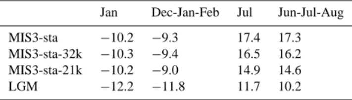
Table 4. Northern Hemisphere – 30◦N to 90◦N – winter and sum-mer SATs (in◦C) for MIS3-sta with 56 ka BP, 32 ka BP and 21 ka BP versus LGM.

Jan Dec-Jan-Feb Jul Jun-Jul-Aug MIS3-sta −10.2 −9.3 17.4 17.3 MIS3-sta-32k −10.3 −9.4 16.5 16.2 MIS3-sta-21k −10.2 −9.0 14.9 14.6

LGM −12.2 −11.8 11.7 10.2

Convergence Zone, which is not the case for the southern side. We argue for a combination of both in a warmer cli-mate with more vigorous NH warming.

4.2 Orbital insolation forcing drives the enhanced season-ality during MIS 3

To further study the impact of insolation on the climate dur-ing MIS3, we perform two sensitivity experiments identical to MIS3-sta, but with orbital parameters for 21 ka BP and 32 ka BP. We have chosen 21 ka for the insolation to be equal to LGM state and 32 ka as, after this date, DO events became less frequent. Together with the 56 ka insolation of the con-trol experiment (MIS3-sta), we nearly cover the full range of Northern Hemisphere insolation changes during MIS 3.

The spatial pattern of the enhanced NH seasonality found in our MIS 3 experiments compared to LGM correlates strongly with the orbital insolation forcing. Here, we show the existence of a causal relation and quantify the climatic impact of this forcing. In MIS3-sta, 56 ka BP insolation re-sults in warmer NH summers in most locations, especially in the high latitudes, while winter temperatures are less af-fected. In the SH, insolation does not differ so strongly between 56 ka BP and 21 ka BP. On Fig. 1 the 60◦N and 60◦S June and December insolation anomalies compared to present-day are depicted for 70–0 ka BP. As can be seen, NH summer insolation rises from a minimum (∼80 ka BP) to a maximum around 60 ka BP, followed by a gradual decline till 40 ka BP and a steady decline until a second minimum around 25 ka BP. At 60◦N, the MIS3-sta June insolation is 39 W m−2more than in the LGM simulation, while the De-cember insolation is 6 W m−2 less, resulting in a seasonal range of 45 W m−2more. When looking at Fig. 3h, we see a seasonal temperature range of more than 10◦_{C larger in}

MIS3-sta than in LGM over the continents at 60◦_N,

suggest-ing a sensitivity of ∼1◦_{C per 4 W m}−2_{additional incoming} solar radiation, and a slight increase over the ocean. (The decrease over the Labrador Sea results from the absence of winter sea-ice, elevating winter temperatures.)

To demonstrate and further quantify the sensitivity of the MIS 3 climate to insolation changes, we compare NH SATs of LGM and MIS3-sta to MIS3-sta-21k and MIS3-sta-32k. At 32 ka BP, the 60◦N June insolation was about 492 W m−2,

so ∼16 W m−2_{less than at 56 ka BP and ∼23 W m}−2_more than at 21 ka BP. In our experiments, we thus expect July SATs to be the highest in sta and the lowest in MIS3-sta-21k. The July SAT anomalies of MIS3-sta-21k and MIS3-sta-32k to MIS3-sta are displayed on Fig. 8. For MIS3-sta-32k, most NH mid- and high-latitude continental locations (and the polar seas) see a significant reduction of

−1◦C to >−10◦C compared to MIS3-sta, whereas some sub-tropical locations feature a slight, but significant warming of +1◦C to +3◦C. Turning to MIS3-sta-21k, we see further cool-ing of the same regions, plus a nearly pan-hemispheric (and possibly inter-hemispheric) expansion of cooling. The 30◦N to 90◦N average January, December-January-February, July and June-July-August SATs are depicted for the four simu-lations in Table 4. Clearly, winter temperatures remain un-affected by the insolation changes. Therefore, winter in-solation changes cannot explain winter temperature differ-ences between LGM and MIS 3. However, July SAT anoma-lies compared to LGM rise from +3.1◦C for MIS3-sta-21k to +4.8◦C for MIS3-sta-32k and +5.7◦C. These temperature differences correspond to 60◦N June insolation anomalies of 0.0%, +3.5% and +6.9% respectively.

The June insolation difference between MIS3-sta and LGM at 60◦N thus results in a July SAT rise of +2.6◦C. The remaining +3.1◦C as well as the increase of January SAT by +2◦C may then be attributed to the remaining forcings, i.e. smaller ice sheets, higher GHG and lower dust concen-trations. Interestingly, NH sea-ice extent, and, more pro-nounced sea-ice volume, on average approach LGM values in our MIS3-sta-21k experiment, again following the inso-lation changes. Moreover, sea-ice extent shows oscillatory behaviour, going from ∼9×106km2to ∼11×106km2, each cycle taking ∼250±100 years, revealing the instability of the Nordic Sea ice cover in this climate state.

The MIS 3 climate seems to have been very sensitive to in-solation changes, at least in the model. Very few reliable ter-restrial seasonal temperature reconstructions are available for MIS 3 in North America, Europe and Asia (Vandenberghe, 1992; Huijzer and Vandenberghe, 1998; Voelker et al., 2002) to allow verification of our model results and the inferred seasonality differences between LGM and MIS 3. Vanden-berghe (1992) did not find evidence for enhanced season-ality during MIS 3 in The Netherlands, with summer tem-peratures only a few degrees warmer than at LGM, while winter temperatures were much reduced, resulting in con-tinuous permafrost. However, Coope (1997), Helmens et al. (2007) and Engels et al. (2007) point out that, during at least one MIS 3 interstadial, warm, close to present-day sum-mer conditions prevailed over Central England (∼18◦C) and northeast Finland (∼13◦C). These warm summers in MIS 3 over mid- and high northern latitudes are consistent with our findings. However, we obtain annual mean temperatures in those regions in our MIS3-sta experiments that are well above 0◦C, whereas the available data suggests much colder stadial conditions, i.e. permafrost over north-western Europe

a) MIS3-sta-21k minus MIS3-sta July SAT anomaly b) MIS3-sta-32k minus MIS3-sta July SAT anomaly

-25 -15 -10 -5 -3 -1 1 3 5 10 15 25 °C

Figure 8

Fig. 8. (a) MIS3-sta-21k minus MIS3-sta and (b) MIS3-sta-32k minus MIS3-sta July SAT anomaly. Grey areas show no significant

differ-ences between the two simulations.

(i.e., annual mean temperature of −4 to −8◦C, Huijzer and Vandenberghe, 1998). The warmer conditions in the model than in the data were also present in the high resolution MIS 3 simulations of Barron and Pollard (2002). Pollard and Bar-ron (2003) suggest that the warm bias might be related to prescribed North Atlantic SSTs, which may have been too elevated to represent MIS 3. In our experiments, however, simulated SSTs remain too high under MIS 3 boundary con-ditions. In the next section, we therefore compare MIS3-sta to MIS3-int to try to disentangle this discrepancy between model and data.

4.3 Comparison of the MIS3-sta and MIS3-int climates While both being clearly warmer than the modelled LGM, the climates of MIS3-sta and MIS3-int differ only very slightly, the latter being at most 1◦C warmer both in sum-mer as in winter (see Fig. 3e, f). Besides slightly larger sea-ice cover in the former (Fig. 7c, f, i, l), the oceans are nearly unaffected by the differences in GHG and dust forc-ings. Our MIS3-int climate may approach interstadial con-ditions fairly well, with a strong Atlantic THC (van Kreveld et al., 2000), relatively little sea-ice cover in the Nordic Seas (Rasmussen and Thomsen, 2004) and warm summer condi-tions over northern Europe (Coope, 1997; Helmens et al., 2007). However, the strong cooling in a stadial and the reduc-tion in deep NADW formareduc-tion (Dokken and Jansen, 1999) – and consequently a slowdown in the Atlantic THC – are not found in our MIS3-sta experiment. We conclude that tem-poral variations in GHG and dust concentrations were less important during MIS 3 than other potential climate forc-ings. It is thus very unlikely that GHG and dust concen-tration changes played a major role in explaining tempera-ture changes during MIS 3. Barron and Pollard (2002) and Pollard and Barron (2003), who did not change CO2forcing from LGM in their simulations, concluded that the temper-ature difference between LGM and MIS 3 conditions regis-tered in the records could not be explained solely by

varia-tions in orbital forcing or in the Scandinavian Ice Sheet size. In contrast, decreasing North Atlantic and Nordic Seas SSTs between a warmer and a colder state to simulate an extended southward distribution of sea ice, explained part of range of temperature differences between the two states.

If GHG and dust forcings can be ruled out as primary drivers of DO climate variability, other factors need to be in-voked to sufficiently alter the THC strength. Ice sheet melt-ing and ice berg calvmelt-ing may hold the key to DO climate variability, if we believe the ongoing hypothesis of THC reg-ulation of Broecker et al. (1985) and numerous other studies. A decrease in SSTs of the North Atlantic and Nordic Seas required to better mimic climatic differences between stadi-als and interstadistadi-als may have been possible with a reduction in THC strength. In this view, our simulations were not in-tended to reproduce the full amplitude of temperature differ-ence between stadials and interstadials. We merely state that setting a realistic climate background should help discrimi-nate mechanisms for DO events, as they were most frequent during MIS 3. With realistic prevailing initial conditions and external forcings we are likely to reduce the uncertainty of the sensitivity of the climate system to parameter changes, i.e. GHG and dust forcings on the one hand, insolation forc-ing on the other.

4.4 Freshwater forcing required to mimic stadials

To investigate the sensitivity of our MIS3-sta climate to freshwater forcing, we perform a third sensitivity experiment in which we perturb the MIS3-sta climate with a strong, ad-ditional freshwater flux in the mid-latitudes of the North At-lantic Ocean to ensure a shut down of the AtAt-lantic THC. From a hysteresis experiment (not presented in this study), we found that in LOVECLIM, the LGM and MIS 3 sensi-tivity of the overall meridional overturning strength to fresh-water perturbation did not differ, with a shutdown occurring at around 0.22Sv. Resumption of the AMOC took place at around 0Sv freshwater forcing. Our MIS 3 experiment with

Sv

a) MIS3-sta Atlantic meridional overturning b) MIS3-HE Atlantic meridional overturning

0 500 1000 1500 2000 2500 3000 3500 4000 4500 5000 5500 0 500 1000 1500 2000 2500 3000 3500 4000 4500 5000 5500 60°S 30°S 0° 30°N 60°N 60°S 30°S 0° 30°N 60°N

Figure 9

Fig. 9. (a) MIS3-sta and (b) MIS3-HE annual mean Atlantic meridional overturning (Sv). The vertical axis represents depth (m), the

horizontal axis gives the latitude. Positive values mean a southward flow of a water body, while negative values imply a northward flow.

collapsed AMOC (MIS3-HE), forced with a constant 0.3Sv freshwater flux is setup as an idealized analogue for a Hein-rich event. To not indefinitely decrease the global ocean’s salinity in this equilibrium run, we allow for a global fresh-water correction. As a result, no global sea level rise due to freshwater input is simulated and the salinity of the North Pa-cific increases. Here we only briefly compare climate condi-tions in the Atlantic sector between MIS3-HE and MIS3-sta, to ensure that the limitation of freshwater correction does not strongly affect our results.

In our MIS3-HE simulation, NADW formation is virtually absent (see Table 3). With the Atlantic MOC shut down, vigorous inflow of intermediate and deep waters from the south takes place (Fig. 9b). Compared to the Atlantic MOC in MIS3-sta (Fig. 9a), the cell transporting NADW disap-pears, with NADW export of less than 2Sv. Conversely, the deep cell reaches the upper layers, with northward inflow of AABW into the Atlantic of more than 9Sv while being less than 4Sv in MIS3-sta. As a consequence of the shutdown Atlantic MOC, the northward oceanic heat flux drops from nearly 0.30PW to −0.46 PW, implying a net southward flux instead (see Table 3).

Associated with this negative northward heat flux in the North Atlantic, a reduction of −4.4◦C in annual mean SST is noted over the entire region, while the Southern Ocean warms up very slightly at best (Table 3). Contrastingly, global mean annual SSTs do not change. The opposite be-haviour of the North Atlantic and Southern Ocean is mirrored by the sea-ice cover. On annual basis, it increases in compa-rable amounts on the NH (+2.8×106km2)as it decreases in the SH (−2.5×106_km2_).

The oceanic response to the freshwater perturbation is re-verberated by the atmosphere. In Fig. 10a, b the July and January SAT anomalies of MIS3-HE minus MIS3-sta are de-picted. In both summer and winter, warming over the

ice-free regions of the Southern Ocean is found, whereas vigor-ous cooling took place over the North Atlantic and much of the NH except for the North Pacific. For instance the winter SAT south and east of Greenland drops by up to −25◦C over the sea-ice. In Europe and over the Arctic Ocean, a cooling of −3◦C down to −10◦C takes place. Even in North Africa and most of Asia a cooling of more than −1◦C is seen. A similar, but slightly weaker cooling occurs during summer. Nonetheless, in some regions slight to substantial warming takes place, +1◦C to +10◦C – e.g. over the Gulf of Alaska and offshore Siberia due to enhanced meridional overturning. While much of the NH winters are chilled to temperatures below or near LGM values – e.g. north-western Europe, be-ing 10◦_{C cooler versus no difference in Central Greenland,}

– the warmer ice-free conditions around eastern Antarctica were echoed by (slighter) warming over much of the SH.

van Huissteden et al. (2003) validated the Stage 3 mod-elling results with permafrost data. Using this method, we find that our MIS3-HE matches the cold surface tempera-tures found in Northern Europe during stadials better than our MIS3-sta. With an inferred southern limit of continuous permafrost in Northern Europe (Huijzer and Vandenberghe, 1998) at around 50–52◦N, the mean annual ground temper-ature must not exceed 0◦C (van Huissteden et al., 2003). In MIS3-sta, we find the 0◦C mean annual SAT isotherm – the best proxy for ground temperature in our model – at around 70◦N in the Nordic Seas, following the Scandinavian Ice Sheet towards the south, between 50◦_{N and 55}◦_{N over}

Germany and around 55◦_{N eastward of Poland (not shown).}

For most locations, the 0◦_{C isotherm lies too far north. In}

contrast, for MIS3-HE we obtain a reasonable match with data, with the 0◦C isotherm lying over Scotland (55–60◦N), Netherlands (50–55◦N), Southern Germany (50◦N) and at around 50◦N over Central and Eastern Europe (not shown).

a) MIS3-HE minus MIS3-sta July SAT anomaly b) MIS3-HE minus MIS3-sta January SAT anomaly

Figure 10

Fig. 10. (a) July and (b) January MIS3-HE minus MIS3-sta SAT anomaly. Grey areas show no significant differences between the two

simulations.

The response of the world oceans to freshwater perturba-tions in the North Atlantic in our model is in line with pre-vious modelling work (e.g. Knutti et al., 2004; Stouffer et al., 2006; Fl¨uckiger et al., 2008) and what is evidenced by proxy reconstructions (e.g. Dokken and Jansen, 1999). The results from our sensitivity study reveal that, in our model, a reduced stadial THC state in a background MIS 3 climate is stable, at least as long as an additional freshwater flux to the North Atlantic is maintained. With an additional 0.3Sv freshwater flux to the North Atlantic, we obtain a climatic pattern similar to other simulations of Heinrich events. This is a consequence of the shutdown of the THC in our model (Fig. 9b). The redistribution of heat causes (slight) warming in the SH, keeping global mean temperatures nearly equal to MIS3-sta or MIS3-int. Such a pattern was seen in the ice cores, and is commonly referred to as the bipolar seesaw (EPICA-community-members, 2006). Over Antarctica, the warmest peaks (2◦C) coincided with the coolest temperatures during stadials in Greenland and HEs in the North Atlantic.

We infer from our results and other studies (e.g. Ganopol-ski and Rahmstorf, 2001) that climate change resembling the observed differences between stadials and interstadials can be obtained when changing the Atlantic THC, through the strength of meridional overturning in the North Atlantic. In our MIS 3 climates, a relatively strong freshwater perturba-tion is required to alter the Atlantic THC. Our findings are corroborated by those of Prange et al. (2002), who found that in an ocean general circulation model, the glacial THC can only remain slowed down or shut down with a strong additional fresh water flux. In the experiments of Ganopol-ski and Rahmstorf (2001) based on an LGM reference cli-mate, imposing a strong freshwater flux of 0.1Sv resulted in a shutdown THC, while only a small negative forcing was imposed to obtain their warm and strong simulated intersta-dial THC mode, respectively small positive forcing for their cold (but strong) simulated stadial THC mode. In the sta-dial mode, convection was confined to the North Atlantic

south of the sea-ice margin, while no NADW was formed at high latitudes. However, the LGM winter sea-ice extent may not have been as southerly in the MIS 3 background cli-mate as during LGM. Consequently, convection would pos-sibly not have been confined to the North Atlantic, but also present in more northern locations as the Nordic Seas as is found in our model. Ganopolski and Rahmstorf (2001) ob-tained Nordic Seas convection in their interstadial mode, as sea-ice retreated northward. More alike their stadial situ-ation, in our MIS3-HE, winter sea-ice cover pushes more southward at some locations in the North Atlantic than in the LGM. In Ganopolski (2003), the simulated MIS 3 sta-dial states strongly resemble that of Ganopolski and Rahm-storf (2001), while using transient MIS 3 forcings as opposed to LGM forcings in the earlier study. Their results imply that the southward extent of sea-ice during stadials does not de-pend on insolation changes or ice sheet size. In our fully three-dimensional model, however, southward winter sea-ice extent is strongly asymmetric between the Labrador Sea and the Nordic Seas, the latter being partly ice-free in the LGM state (Roche et al., 2007). Compared to the LGM, in our model the sea-ice cover in MIS3 is less extensive, with a partly ice-free Labrador Sea in winter and a more northerly positioned sea-ice edge in the Nordic Seas. This implies that the sea-ice cover and the ocean state depend on varying glacial insolation and ice sheet size changes.

Our MIS 3 climates are warmer than the LGM, with con-vection sites and sea-ice extent that are more similar to present-day climate. The sensitivity of the THC to fresh-water forcing is also expected to be different from LGM. For this reason, we argue that LGM should not be used to simulate DO events. Rather, one should start from a cli-mate state obtained under MIS 3 boundary conditions. With Labrador Sea deep convection in our MIS3 simulations, the east-west structure of the Atlantic Thermohaline Circulation was different from the LGM case. The regional climate of the Labrador Sea area and surroundings (including Greenland)

could become more sensitive to meltwater perturbations. In-vestigating this sensitivity is beyond the scope of the paper and is the subject of an ongoing study.

4.5 Perspectives

Knowing that deep convection perturbation through a fresh-water flux in the Labrador, the Nordic Seas and the North Atlantic may trigger transitions from milder to colder glacial conditions, freshwater hosing experiments have long con-quered the palaeoclimate modelling community. However, many, if not all experiments investigating the nature of DO events have been setup with very crude forcings, namely present-day, pre-industrial or LGM. Moreover, due to com-putational costs, only simple models have been used so far in transient experiments of glacial abrupt climate change (Ganopolski, 2003). We have shown that in a fully three-dimensional model of intermediate complexity, the base cli-mate varies greatly with different forcings and boundary con-ditions. In a test to estimate atmospheric CO2 concentra-tions that allow simulating climate shifts resembling the DO events, Wang and Mysak (2006) found that they only oc-curred under MIS 3 values. By applying realistic MIS 3 forcings, we discovered relatively low climate sensitivity to GHG forcing, but a high sensitivity to insolation forcing. The mechanism behind the ice sheet melting may be rein-terpreted as warmer summers during MIS 3 could have pro-vided a baseline melt water flow to the North Atlantic. In this case, freshwater forcing into the North Atlantic would not only form a theoretical exercise, but would be physically consistent.

A first attempt at modelling glacial abrupt climate events in a physically consistent way was undertaken by Ganopol-ski (2003), Claussen et al. (2005) and Jin et al. (2007) in an earth system model of intermediate complexity incorporating a two-dimensional ocean model. By applying transient MIS 3 forcings, they obtain a Greenland temperature evolution not unlike the observed changes associated with DO events. In their model, the simulated DO events are a robust phe-nomenon under a broad range of NH ice sheet volume. How-ever, their exercise could be improved by applying all known boundary condition changes. Furthermore, employing three-dimensional Ocean General Circulation Models would pro-vide insight on longitudinally asymmetric changes in over-turning, e.g. the presence or absence of Labrador Sea con-vection.

No great source of freshwater to the North Atlantic would have been present during stadials without HEs, however (e.g. Bond et al., 1993; van Kreveld et al., 2000). This is in contrast with certain sites in the Nordic Seas (Rasmussen et al., 1996; Rasmussen and Thomsen, 2004) where planktonic and benthic δ18O levels in combination with IRD layers dicate a freshwater source during all cooling phases from in-terstadials to stadials during MIS 3. Using such information, we may setup more realistic freshwater hosing experiments,

for instance by selecting key regions for the freshwater input. Recently, it has been shown that freshwater forcing in differ-ent regions causes differdiffer-ent response of the oceanic circula-tion (Roche and Renssen, 2008). We thus propose to design physically consistent DO experiments, by carefully setting up the model with realistic forcings.

5 Conclusions

In our MIS 3 climate simulations with the three-dimensional earth system model LOVECLIM, we find a warmer base climate than that of LGM simulated with the same model. Boundary conditions were different during MIS 3 than at LGM, notably insolation, ice sheet configuration, atmo-spheric greenhouse gases and dust concentrations, all leading to a positive forcing. Our main findings are:

– With smaller Northern Hemisphere ice sheets, higher greenhouse gases and lower dust concentration, MIS 3 mean annual temperatures are higher than LGM (glob-ally +1.7◦C for MIS3-sta and +2.0◦C for MIS3-int). – Orbital insolation forcing leads to enhanced Northern

Hemisphere seasonality, with mainly warmer summers due to an increase of summer insolation, whereas win-ter insolation does not change substantially. North-ern hemisphere mean July temperature anomalies com-pared to LGM are +3.5◦_{C for MIS3-sta (+5.7}◦_C

be-tween 30◦N and 90◦N) and +3.8◦C for MIS3-int. The sensitivity of the MIS 3 climate to insolation changes is relatively high (up to 1◦C per 4 W m−2). June insolation is 39 W m−2 higher in MIS3-sta than in LGM, which explains about half (2.5◦C between 30◦N and 90◦N) of the July temperature differences.

– With only greenhouse gases and dust concentration forcing different between a colder (MIS3-sta) and a warmer (MIS3-int) experiment, large temperature dif-ferences found in data between cold stadials and mild interstadials over Europe and the North Atlantic region cannot be explained. The different forcings between the two states result in a global temperature difference of 0.3◦_{C in annual means, as well as in January and July}

(and less than 1◦_{C over Europe and the North Atlantic}

region). These small differences point to a low sensi-tivity of the MIS 3 climate to the reconstructed green-house gases and dust concentration changes during that period. In our simulations, the MIS3-sta climate is not cold enough to represent stadial conditions in Europe, whereas MIS3-int better mimics interstadial climate. – The overall strength of the Atlantic meridional

over-turning circulation does not differ substantially between LGM and MIS 3. However, in MIS 3 convection sites

shift more northward in the Atlantic with deep tion found in the Labrador Sea and enhanced convec-tion taking place in the Nordic Seas. Both areas are not covered by perennial sea-ice in our MIS 3 simulations. With Labrador Sea deep convection in our MIS 3 simu-lations but not in the LGM experiments, the configura-tion of the Atlantic Thermohaline Circulaconfigura-tion is differ-ent between MIS 3 and LGM. Since the Labrador Sea is close to the Laurentide and Greenland ice sheets, it can be expected that deep convection here is susceptible to variations in freshwater input. This could have im-portant implications for the climate over the Northwest Atlantic region and downwind areas (such as Southern Greenland). Hence, an LGM state should not be used to simulate DO events.

– If we add 0.3 Sv of freshwater to the North Atlantic Ocean in our stadial simulation, we shut down the Atlantic thermohaline circulation, leading to a much colder climate over Europe and the North Atlantic re-gion. The annual mean temperatures in these two regions are 7.4◦C, respectively 6.9◦C colder than in MIS3-sta. The simulated cooling leads to a better tem-perature match with permafrost reconstructions over Europe regarding stadials than in our MIS3-sta simula-tion. This simulation compares to previous glacial sim-ulations with shutdown thermohaline circulation, with freshwater forcing explaining most of the temperature difference between modelled stadials and interstadials. Our findings contribute to understanding the mechanisms be-hind Dansgaard-Oeschger events. In our model, the cold state with freshwater forcing is more consistent with ob-served stadial climate than the one without. In this view, stadials would be unstable, colder intervals, while intersta-dial climate would be closer to our modelled MIS 3 equilib-rium state. This MIS 3 equilibequilib-rium state is generally warmer than the LGM. We need to design physically consistent cli-mate modelling experiments based on boundary conditions that are realistically representing the period of interest. We confirm once more that insolation differences in glacial peri-ods are important, which we have shown for MIS 3 as com-pared to LGM.

Acknowledgements. This work is a contribution to the

RESOLuTION-project (ESF EUROCORES on EuroCLIMATE program). C. J. V. M. was sponsored by the Netherlands Organ-isation for Scientific Research (NWO), under contract number 855.01.085. D. M. R. was sponsored by the NWO under contract number 854.00.024. We wish to thank referee A. Ganopolski and an anonymous referee for their thorough review, the manuscript greatly benefited from their suggestions.

Edited by: D.-D. Rousseau

References

Alfano, M. J., Barron, E. J., Pollard, D., Huntley, B., and Allen, J.: Comparison of climate model results with European vegetation and permafrost during Oxygen Isotope Stage Three, Quaternary Res., 59, 97–107, 2003.

Barron, E. J. and Pollard, D.: High-resolution climate simulations of oxygen isotope stage 3 in Europe, Quaternary Res., 58, 296– 309, 2002.

Berger, A. L.: Long-term variations of daily insolation and Quater-nary climatic changes, J. Atmos. Sci., 35, 2363–2367, 1978. Berger, A. and Loutre, M. F.: Insolation values for the climate of the

last 10 million years, Quaternary Sci. Rev., 10, 297–317, 1991. Bond, G., Broecker, W., Johnsen, S., McManus, J., Labeyrie, L.,

Jouzel, J., and Bonani, G.: Correlations between climate records from North Atlantic sediments and Greenland ice, Nature, 365, 143–147, 1993.

Broecker, W. S., Peteet, D. M., and Rind, D.: Does the ocean-atmosphere system have more than one stable mode of opera-tion? Nature, 315, 21–26, doi:10.1038/315021a0, 1985. Broecker, W. S.: Massive iceberg discharges as triggers for global

climate change, Nature, 372, 421–424, 1994.

Broecker, W. S., Peng, T.-H., Jouzel, J., and Russell, G.: The mag-nitude of global fresh-water transports of importance to ocean circulation, Clim. Dynam., 4, 73–79, 1990.

Brovkin, V., Ganopolski, A., and Svirezhev, Y.: A continuous climate-vegetation classification for use in climate-biosphere studies, Ecol. Model., 101, 251–261, 1997.

Chappell, J.: Sea level changes forced ice breakouts in the Last Glacial cycle: new results from coral terraces, Quaternary Sci. Rev., 21, 1229–1240, 2002.

Claquin, T., Roelandt, C., Kohfeld, K., Harrison, S., Tegen, I., Pren-tice, I., Balkanski, Y., Bergametti, G., Hansson, M., Mahowald, N., Rodhe, H., and Schulz, M.: Radiative forcing of climate by ice-age atmospheric dust, Clim. Dynam., 20, 193–202, 2003. Clark, P. U., Hostetler, S. V., Pisias, N. G., Schmittner, A., and

Meissner, K. J.: Mechanisms for an ∼7-kyr Climate and Sea-Level Oscillation During Marine Isotope Stage 3, in: Ocean Cir-culation: Mechanisms and impacts—Past and future changes of meridional overturning, edited by: Schmittner, A., Chiang, J. C. H., and Hemming, S. R., American Geophysical Union, Wash-ington, DC, USA, 209–246, 2007.

Claussen, M., Ganopolski, A., Brovkin, V., Gerstengarbe, F.-W., and, Werner, P.: Simulated global-scale response of the climate system to Dansgaard/Oeschger and Heinrich events, Clim. Dy-nam., 21, 361–370, 2003.

Coope, G. R., Gibbard, P. L., Hall, A. R., Preece, R. C., Robinson, J. E., and Sutcliffe, A. J.: Climatic and environmental recon-structions based on fossil assemblages from Middle Devensian (Weichselian) deposits of the river Thames at South Kensing-ton, Central London, UK, Quaternary Sci. Rev., 16, 1163–1195, 1997.

Dansgaard, W., Johnsen, S. J., Clausen, H. B., Dahl-Jensen, D., Gundestrup, N. S., Hammer, C. U., Hvidberg, C. S., Steffensen, J. P., Sveinbj¨ornsdottir, A. E., Jouzel, J., and Bond, G.: Evidence for general instability of past climate from a 250-kyr ice-core record, Nature, 364, 218–220, 1993.

Dokken, T. and Jansen, E.: Rapid changes in the mechanism of ocean convection during the last glacial period, Nature, 401, 458–461, 1999.