The 1985 southern hemisphere mid-latitude total column ozone anomaly

HAL Id: hal-00302810

https://hal.archives-ouvertes.fr/hal-00302810

HAL is a multi-disciplinary open access

archive for the deposit and dissemination of sci-entific research documents, whether they are pub-lished or not. The documents may come from teaching and research institutions in France or abroad, or from public or private research centers.

L’archive ouverte pluridisciplinaire HAL, est destinée au dépôt et à la diffusion de documents scientifiques de niveau recherche, publiés ou non, émanant des établissements d’enseignement et de recherche français ou étrangers, des laboratoires publics ou privés.

The 1985 southern hemisphere mid-latitude total

column ozone anomaly

G. E. Bodeker, H. Garny, D. Smale, M. Dameris, R. Deckert

To cite this version:

G. E. Bodeker, H. Garny, D. Smale, M. Dameris, R. Deckert. The 1985 southern hemisphere mid-latitude total column ozone anomaly. Atmospheric Chemistry and Physics Discussions, European Geosciences Union, 2007, 7 (3), pp.7137-7169. �hal-00302810�

ACPD

Printer-friendly Version Interactive Discussion Atmos. Chem. Phys. Discuss., 7, 7137–7169, 2007

www.atmos-chem-phys-discuss.net/7/7137/2007/ © Author(s) 2007. This work is licensed

under a Creative Commons License.

Atmospheric Chemistry and Physics Discussions

The 1985 southern hemisphere

mid-latitude total column ozone anomaly

G. E. Bodeker1, H. Garny2, D. Smale1, M. Dameris3, and R. Deckert3

1

National Institute of Water and Atmospheric Research, Lauder, New Zealand

2

Meteorological Institute, University of Munich, Munich, Germany

3

DLR-Institut f ¨ur Physik der Atmosph ¨are, Oberpfaffenhofen, Germany Received: 5 April 2007 – Accepted: 14 May 2007 – Published: 25 May 2007 Correspondence to: G. E. Bodeker (g.bodeker@niwa.co.nz)

ACPD

Printer-friendly Version Interactive Discussion

Abstract

One of the most significant events in the evolution of the ozone layer over southern mid-latitudes since the late 1970s was the large decrease observed in 1985. This event remains unexplained and most state-of-the-art atmospheric chemistry-transport mod-els are unable to reproduce it. In this study, the 1985 southern hemisphere mid-latitude

5

total column ozone anomaly is analyzed in detail based on observed daily total column ozone fields, stratospheric dynamical fields, and calculated diagnostics of stratospheric mixing. The 1985 anomaly appears to result from a combination of (i) an anomaly in the meridional circulation resulting from the westerly phase of the equatorial quasi-biennial oscillation (QBO), (ii) weaker transport of ozone from its tropical mid-stratosphere

10

source across the sub-tropical barrier to mid-latitudes related to the particular phas-ing of the QBO with respect to the annual cycle, and (iii) a solar cycle induced local reduction in ozone. The results based on observations are compared and contrasted with analyses of ozone and dynamical fields from the ECHAM4.L39(DLR)/CHEM cou-pled chemistry-climate model (hereafter referred to as E39C). Equatorial winds in the

15

E39C model are nudged towards observed winds between 10◦_{S and 10}◦_{N and the}

ability of this model to produce an ozone anomaly in 1985, similar to that observed, confirms the role of the QBO in the anomaly.

1 Introduction

Total column ozone over southern mid-latitudes has decreased since the early 1980’s.

20

However, this decrease has not occurred as a purely monotonic decline but rather as a number of stepwise decreases superimposed on a background linear decline. Perhaps the largest of these stepwise decreases occurred in 1985 when total column ozone over southern mid-latitudes decreased by up to 30 Dobson Units (DU; 1 DU = 2.69×10

16

molecules/cm2) depending on location. This feature has been commented

25

ACPD

Printer-friendly Version Interactive Discussion state-of-the-art chemistry-transport models and remains largely unexplained (WMO,

2003).

Potential explanations for the 1985 ozone anomaly are: 1. In situ depletion of ozone over southern mid-latitudes. 2. Export of ozone depleted air from Antarctica.

5

3. A reduction in mid-latitude ozone due to a QBO induced change in the strength of the meridional circulation.

4. Anomalously weak transport of ozone from its tropical source, across the sub-tropical barrier, to mid-latitudes. This could result from unforced inter-annual vari-ability in the frequency of mixing events or from the QBO itself (thereby creating

10

a second order dependence on the QBO).

5. Reduced mid-latitude ozone concentrations due to a minimum in the solar cycle. A combination of these processes may also be possible. While the El Ni ˜no Southern Oscillation (ENSO) is known to drive changes in total column ozone in the southern hemisphere in winter (Randel and Cobb, 1994), the Southern Oscillation Index (the

15

normalized Tahiti minus Darwin sea-level pressure) was close to zero through 1984, 1985 and 1986. Therefore we have not considered ENSO as a potential explanatory factor for the 1985 ozone anomaly.

The first option is highly unlikely as there are no documented sudden and rapid in-creases in ozone depleting substance concentrations nor of rapid changes in southern

20

mid-latitude stratospheric chemistry over this period.

With regard to option 2, the vortex period averaged ozone mass deficit over Antarc-tica in 1985 was approximately 2.5 times larger than in 1984 (4.63×10

9

kg in 1985 cf. 1.85×10

9

kg in 1984) and greater than any previous year (Huck et al.,2005). While it is unlikely that this ozone depleted air over Antarctica would have affected mid-latitudes

25

ACPD

Printer-friendly Version Interactive Discussion much before the breakdown of the polar vortex, if there was considerable diabatic

de-scent inside the vortex during this period, air depleted in ozone may have been trans-ported down into the lowermost stratosphere, below the base of the vortex. Transport along isentropic surfaces could have advected the descended anomaly out to mid-latitudes. However, previous analysis of total column ozone anomalies (see Fig. 6b of

5

Kinnersley and Tung,1998) shows that the anomaly appears in the first half of 1985

at sub-tropical latitudes and then propagates poleward, reaching the Antarctic in Octo-ber/November of that year. This suggests that the anomalously large Antarctic ozone depletion in 1985 was caused in part by an equatorial anomaly advected poleward rather than the driver of the anomaly itself.

10

Kinnersley and Tung (1998) showed that by forcing an interactive

chemical-dynamical model of the stratosphere with observed Singapore zonal winds and with the observed daily varying planetary wave heights just above the tropopause, much of the observed interannual variability in monthly mean total column ozone globally could be reproduced. Similar to the approach used in the E39C model (see Sect.2), the zonal

15

winds between 10 and 70 hPa and between 10◦_{S and 10}◦_{N were relaxed towards the}

observed Singapore winds with a time constant of 1 day. The best correlations were found within 50◦ _{of the equator during winter and autumn in both hemispheres (the}

period when wave induced transport of ozone from the tropics to higher latitudes is greatest), suggesting that the fourth possibility listed above might be more likely. In

20

this model, the propagation of the ozone anomaly from equatorial to higher latitudes occurred only in the southern hemisphere. However,Kinnersley and Tung(1998) did not use observed planetary wave amplitudes in the southern hemisphere but rather a repeating annual (July 1980 to June 1981) cycle of wave amplitudes since “use of the observed interannually varying waves gave unrealistic results”. Therefore, any

plane-25

tary wave induced equator to pole advection anomaly in 1985 would not be faithfully reproduced in their model. Furthermore,Kinnersley and Tung(1999) showed that the mid-latitude QBO signal in ozone results primarily from the direct QBO modulation of the meridional circulation and, to a lesser extent, QBO modulation of mid-latitude

ACPD

Printer-friendly Version Interactive Discussion planetary wave activity. As opposed toGray and Pyle(1989), who modelled the

extra-tropical QBO signal in ozone as a poleward advection and diffusion of the QBO induced tropical ozone anomaly,Kinnersley and Tung(1999) found that diffusion by planetary waves actually reduces the mid-latitude ozone anomaly by spreading it to lower and high latitudes. That said, reduced diffusion by planetary waves and/or reduced

trans-5

port of ozone from its tropical source region to mid-latitudes, would exacerbate the anomaly as the smoothing effects of the mixing would be reduced. Using Lyapunov exponents as a measure of mixing,Bowman(1993) showed anomalously weak mixing between the tropics and southern mid-latitudes in 1985.

Kinnersley and Tung (1998) proposed a positive feedback that would amplify

neg-10

ative ozone anomalies caused by the QBO i.e. if the Antarctic stratosphere is colder than usual due to the QBO (Lait et al.,1989) ozone depletion will be enhanced as a result of greater polar stratospheric cloud formation. Reduced ozone will reduce solar heating which will strengthen the circumpolar vortex, decrease planetary wave activity, and so reduce mixing of ozone from lower latitudes and further reduce ozone levels. It

15

should be noted that ozone responds not only to the secondary circulation associated with the QBO but also to the temperature variations because of the strong dependence of chemical loss rates on temperature (Lee and Smith,2003). This suggests that the third and fourth possibilities listed above, working in tandem, and possibly with local ozone levels further reduced by a minimum in the solar cycle (McCormack and Hood,

20

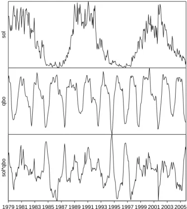
1996;Soukharev and Hood,2006), could explain the 1985 mid-latitude anomaly. It is

interesting to note that the product of a 50 hPa QBO signal and a solar activity index (Fig.1) shows anomalously low values through most of 1985 and early 1986, as well as 1995 and 1997 (which also showed anomalously low southern mid-latitude ozone, see Sect.3.1).

25

ACPD

Printer-friendly Version Interactive Discussion

2 The E39C model

A full description of the E39C model is provided inDameris et al.(2005) andDameris

et al. (2006). The features of the model relevant to this study are summarized in this section. The model has a horizontal resolution of T30, with 39 layers from the surface to an upper layer centered at 10 hPa. Heating and photolysis rates are sensitive to the

5

three-dimensional distributions of the radiatively active gases (O₃, CH₄, N₂O, H₂O, and CFCs), and clouds, so that changes in atmospheric composition affect atmospheric temperatures and hence transport. Observed sea surface temperatures and sea ice cover (update ofRayner et al.,2003), and observed greenhouse gases and CFC con-centrations (WMO,2003), provide the model boundary conditions. The 11-year solar

10

cycle affects both heating rates and photolysis rates of chemical species. The impact of solar activity changes on short-wave heating rates is prescribed in two spectral in-tervals by varying the solar constant. Continuum scattering, grey absorption, water vapor and uniformly mixed gas transmission functions and ozone transmission are all considered (Dameris et al., 2005). The effects of changes in solar activity on

pho-15

tolysis rates are parameterized in 8 spectral intervals (between 178.8 and 752.5 nm) according to 10.7 cm solar flux measurements (see Fig. 1). The spectral distribution of changes in extra-terrestrial solar flux is based on Lean et al. (1997). The effects of solar activity at altitudes above 30 km are accounted for by prescribing changes in total nitrogen, obtained from a transient simulation of a 2-D model (Br ¨uhl and Crutzen,

20

1993), as a model upper boundary condition. The QBO is forced by linear relaxation of the equatorial zonal winds in the lower stratosphere toward observed zonal wind pro-files. The effects of past major volcanic eruptions (Agung in 1963, El Chich ´on in 1982, and Pinatubo in 1991) are also included.

ACPD

Printer-friendly Version Interactive Discussion

3 The evidence

3.1 Temporal and spatial pattern of the anomaly

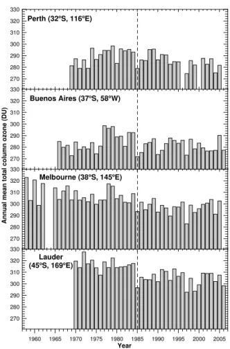
The temporal context of the 1985 anomaly is shown in Fig.2where long-term annual mean time series of total column ozone from 4 locations are plotted.

The annual means at the 4 sites were calculated from Dobson spectrophotometer

5

measurements obtained from the World Ozone and UV Data Center (WOUDC), re-quiring 5 daily values for a monthly mean to be valid, at least 8 monthly means for an annual mean to be valid, and with corrections based on a monthly mean climatology to correct for temporal seasonal biasing in these calculations. Missing values result from these criteria not being met (e.g. only Lauder and Buenos Aires have values for 2006).

10

These long-term time series show that the 1985 anomaly represents one of the largest year-to-year changes in annual mean ozone on record and is a key characteristic of long-term changes in ozone over southern mid-latitudes. 1997 also shows very low annual mean total column ozone at all 4 sites and this feature has been discussed by

Connor et al.(1999).

15

An earlier analysis of changes in mid-latitude ozone mass indicated that the reduc-tions in southern mid-latitude ozone in 1985 and 1997 were accompanied by increases in ozone over northern mid-latitudes (see Fig. 5 ofBodeker et al.,2001). The ozone mass time series plotted inBodeker et al. (2001) have been updated and differences between deseasonalised mid-latitude (30◦_–60◦_{) ozone mass values have been} calcu-20

lated based on both the NIWA combined total column ozone data base (Bodeker et al.,

2005) and output from the E39C run (see Fig.3).

The years of 1985, 1997 and 2006 (see discussion below for why 2006 is consid-ered to be similar to 1985 and 1997) are characterized by increases in the differences between northern and southern mid-latitude ozone mass anomalies that build through

25

the year. At the beginning of the year the southern mid-latitudes have a positive ozone mass anomaly with respect to the northern mid-latitudes but by the end of the year the situation is reversed. This seasonal evolution is seen in both the observations and in

ACPD

Printer-friendly Version Interactive Discussion the E39C model output and is explored further in Sect.3.3.

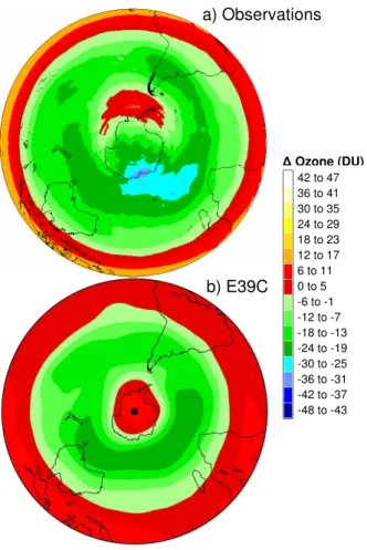
To show more clearly the full spatial structure of the 1985 anomaly, differences be-tween the southern hemisphere annual mean total column ozone, calculated using Nimbus 7 TOMS (Total Ozone Mapping Spectrometer) total column ozone fields are displayed in Fig.4together with the analogous difference field obtained from the E39C

5

run.

Regions coloured green and blue show where total column ozone in 1985 was lower than in 1984 while regions coloured red and yellow show where total column ozone in 1985 was higher than in 1984. Both the observed and modelled difference fields are characterized by a ring of positive anomalies within ∼15◦ _{of the equator, indicative of} 10

the influence of the equatorial QBO (Gray and Pyle,1989), surrounding a large extra-tropical region of predominantly negative anomalies. A wave 1 structure exhibiting weak positive anomalies south of South America, and large negative anomalies ex-ceeding –30 DU close to the perimeter of the Antarctic continent between South Africa and Australia, is superimposed on the observed anomaly field. In contrast, a much

15

weaker wave structure is seen in the E39C anomaly field and with positive anomalies over Antarctica. Care must be taken when interpreting high latitude differences be-tween the two fields plotted in Fig.4because of potential temporal biasing i.e. if from May to August ozone over Antarctica in 1985 was in fact higher than in 1984 this would not be fully accounted for in the observations since TOMS is unable to measure ozone

20

in regions of polar darkness.

The origin of the wave 1 structure in the observed anomalies can be discerned from Fig.5where daily 100 hPa geopotential height and temperature fields at 12:00 UT from the National Centers for Environmental Prediction/National Center for Atmospheric Re-search (NCEP/NCAR) reanalyses (Kistler et al.,2001) were used to calculate the

an-25

nual mean geopotential height and temperature differences from 1984 to 1985.

Both difference fields show a clear wave 1 pattern where reduced geopotential heights and lower temperatures in 1985 compared to 1984 are approximately collo-cated with the region of reduced ozone while areas of raised geopotential height and

ACPD

Printer-friendly Version Interactive Discussion higher temperatures are approximately collocated with the region of enhanced ozone

near the southern part of South America. This indicates that the wave 1 pattern seen in Fig.4a results from an underlying change in the synoptic scale wave structure over the southern mid-latitudes from 1984 to 1985. Further discussion of the interannual variability in southern mid-latitude wave forcing is presented in Sect.3.5.

5

3.2 Changes in the frequency of high and low ozone events

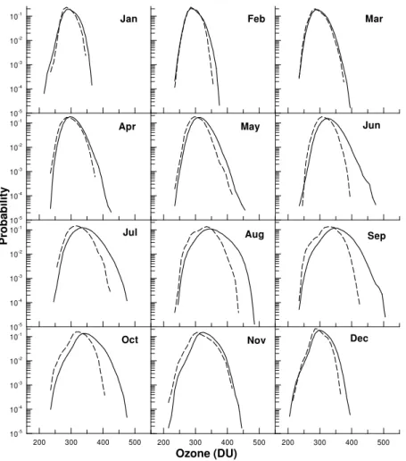
To show more clearly the changes in ozone that occur each month in 1985 compared to the mean of the 1980s decade, monthly probability distribution functions (PDFs) have been calculated from daily 1.25◦ _{longitude by 1.0}◦ _{latitude total column ozone fields}

from Nimbus 7 TOMS over 30◦_{S to 60}◦_{S. The monthly PDFs for 1985 are compared} 10

against the 1980–1989 (but excluding 1985) climatological mean PDFs in Fig.6. Throughout 1985 it appears that the likelihood of measuring high ozone values de-creased rather than the likelihood of lower ozone values increasing. This is particu-larly apparent in spring (September and October) when, in 1985, ozone values above 450 DU were hardly ever encountered. This suggests that the 1985 anomaly resulted

15

from a reduction in highest ozone values rather than an increase in lowest ozone val-ues. The ozone PDFs calculated from the E39C total column ozone fields are shown in Fig.7. These too show that the 1985 anomaly is characterized by reductions in the probability of high ozone values rather than increases in the probability of low ozone values. This provides further evidence that it is unlikely that the 1985 anomaly results

20

from export of ozone depleted air from Antarctica since this would have increased the probability of very low ozone values.

3.3 Inter-hemispheric structure of the anomaly

Principal component analysis has been used to investigate whether the 1985 southern mid-latitude anomaly is related to any large scale pattern of variability in global ozone.

25

Monthly mean, zonal mean (1◦_{zones) total column ozone time series were generated}

ACPD

Printer-friendly Version Interactive Discussion from the NIWA combined total column ozone data base. Similar time series were

generated from the E39C runs where ozone was interpolated to 1◦ _{resolution. To}

form anomaly time series with respect to the period before significant ozone depletion began, mean annual cycles calculated from 1980 to 1983 were subtracted from the time series at each latitude.

5

Spatial and temporal modes of variability in the zonal mean anomaly time series were calculated separately for each month by decomposing the area weighted anomaly co-variance matrix by principle component analysis (Preisendorfer,1988). The analysis was performed individually for each month so as to maximize the latitudinal coverage (satellite coverage of polar regions in winter is limited) and since patterns of

variabil-10

ity were expected to be seasonally dependent. The decomposed temporal modes were normalized so that the variance of each temporal mode was 1.0. The normal-ized temporal modes (principal components; PCs) were projected onto the zonal mean anomalies to generate the spatial modes (empirical orthogonal functions; EOFs). The EOFs were then area de-weighted.

15

For the month of November, the PC time series for the third EOF identified a merid-ional pattern in ozone changes that maximized in 1985, 1997 and 2006 which were years of anomalously low southern mid-latitude ozone (see Fig.2). The first and sec-ond EOFs, not shown here, reflect November trends in total column ozone and year-to-year variability in the timing of the vortex breakdown, respectively. The third EOF

20

pattern is plotted together with its PC time series in Fig.8.

For the E39C model, it was the second EOF that most closely resembled the third EOF based on measurements, and this too is plotted in Fig.8. The PC time series based on measurements and model output are highly correlated (R2=0.59). The third EOF explains approximately 3% of the total variance in the measured zonal mean

25

ozone while the second EOF explains approximately 12% of the total variance in the modelled zonal mean ozone. PC time series based on measurements and on model output identify 1985 and 1997 as anomalous, and the measurements, which extend to 2006, also show 2006 to be anomalous. The measured and modelled EOF patterns

ACPD

Printer-friendly Version Interactive Discussion both show negative ozone anomalies in southern mid-latitudes and the EOF pattern

based on measurements suggests that these negative anomalies occur in conjunction with positive total column ozone anomalies in northern mid-latitudes. The positive anomalies occurs at higher northern latitudes in the model.

This dipole pattern is consistent with the mid-latitude ozone mass differences plotted

5

in Fig. 3. Because the hemispheric ozone mass differences appear to accumulate through the year, the principal component analysis results for November, close to when these differences maximize, show this pattern most clearly.

3.4 Associated anomalies in stratospheric mixing

As outlined in Sect.1, the fourth possible explanation for the 1985 ozone anomaly is an

10

anomaly in the transport of ozone from the tropics to mid-latitudes. Transport is deter-mined by the amount of mixing between the tropics and mid-latitudes, which can vary from year to year and therefore change the amount of ozone rich air transported out of the tropics to higher latitudes. To diagnose the degree of mixing over the southern hemisphere, Lyapunov exponents were calculated as was done inBowman(1993). A

15

description of Lyapunov exponents, their use in diagnosing atmospheric mixing, the algorithm for their calculation, and an analysis of uncertainties is presented in detail

in Garny et al. (2007). Briefly, Lyapunov exponents measure the separation of two

trajectories with time from initially nearby starting points. The exponents are related to the local stretching deformation of the fluid following an air parcel (Bowman,1993).

20

Divergent velocity fields produce positive Lyapunov exponents, while convergent fields produce negative exponents.

Two dimensional (latitude and longitude) Lagrangian trajectories were computed on isentropic surfaces using a standard 4th order Runge-Kutta integration scheme (Press

et al.,1989) applied at 1 h integration intervals to 6 hourly 2.5◦

×2.5◦NCEP/NCAR wind

25

fields, and 12 hourly E39C model wind fields, on the 450, 550 and 650 K isentropes. Trajectories within 20◦ _{of the poles are transformed to a Cartesian coordinate system}

to avoid the singularity at the pole which occurs when prescribing winds using zonal 7147

ACPD

Printer-friendly Version Interactive Discussion and meridional components.

To determine the mixing between the tropics and mid-latitudes, Lyapunov exponents were calculated for each month from 1980 to 1989 based on 30 day trajectories for both measured and modelled data. The starting positions for the trajectories were specified at 2◦ _{longitude spacing and 1}◦ _{latitude spacing covering the whole of the} 5

southern hemisphere. Examples of the calculated trajectories as well as various fields and zonal mean time series of the resultant Lyapunov exponents are shown inGarny

et al. (2007). Southern hemisphere anomalies in monthly Lyapunov exponents (not shown here), calculated by subtracting the mean annual cycle from the time series at each degree of latitude, identify 1985 as having anomalously weak mixing from the

10

equator to poleward of 40◦_{S. Therefore, to highlight the extent to which mixing between}

the tropics and mid-latitudes was unusual in 1985, the monthly Lyapunov exponents, based on both NCEP/NCAR wind fields and E39C wind fields, were averaged between the equator and 40◦_{S for all three isentropic levels. The values for 1985 are compared}

with the 1980–1989 climatology (but excluding 1985) in Fig.9.

15

At 450 K the measured and modelled Lyapunov exponents show very different sea-sonal structure. In the observations, highest mixing occurs in January and February (with a secondary maximum in winter) while in the E39C model, highest mixing oc-curs from July to September. Furthermore, the observations show weaker than usual mixing through most of 1985 and particularly in September and October. In contrast,

20

the model shows significantly weaker mixing only during the first 4 months of 1985. At 550 K, both the measurements and the model show mixing maximizing in winter (June to August), but with generally weaker mixing in the model than in the measurements. The observations show anomalously weak mixing in 1985 from May to September while the model shows moderately weaker mixing through the first half of the year. At

25

650 K, mixing also maximizes in the winter, both in the observations and in the model. As at 550 K, the equator to mid-latitude mixing in the model is weaker than in the obser-vations. While the observations show no anomalously low mixing in 1985 at 650 K, the model does show weaker mixing through much of the middle of the year. Therefore,

ACPD

Printer-friendly Version Interactive Discussion while both measurements and model show a mixing anomaly in 1985, the anomaly

occurs at higher altitudes in the model than in observations. 3.5 Associated anomalies in wave forcing

Since mixing in the mid-latitude surf zone is driven primarily by planetary scale wave breaking, it is natural to consider whether planetary wave activity in 1985 was

anoma-5

lous. To this end daily 20 hPa geopotential height wave amplitudes at 60◦_{S have}

been calculated from NCEP/NCAR fields and from 20 hPa geopotential height fields extracted from the E39C model. A discrete Fourier transform has been used to calcu-late the wave amplitudes for zonal waves 1 to 5. Winter-time (mid-July to the end of November) means of these wave amplitudes are plotted in Fig.10.

10

The measured wave amplitudes in 1985 show a suppression of energy in wave 2 and an increase of energy in wave 3. The wave 3 amplitude in 1985 exceeds all other years. The E39C wave amplitudes also show a suppression of energy in wave 2 but no concomitant increase of energy in wave 3. The increasing wave 1 amplitudes in the NCEP/NCAR 20 hPa geopotential height fields suggest that mixing in the southern

15

mid-latitude surf zone should have increased over this period. Garny et al. (2007) report increasing mixing on the 450 K isentrope through much of the mid-latitudes of the southern hemisphere from 1979 to 2005. The E39C wave 1 amplitudes show a much weaker positive trend, if any, from 1979 to 1999.

4 Discussion

20

A number of lines of evidence were presented above which provide clues as to the origin of the 1985 southern mid-latitude total column ozone anomaly. A discussion of this evidence and the conclusions drawn are presented below.

The spatial pattern of ozone change from 1984 to 1985 (see Fig.4) was evocative of QBO influence. The fact that the E39C coupled chemistry-climate model, whose

25

ACPD

Printer-friendly Version Interactive Discussion equatorial winds are nudged towards observed winds, was able to capture many of the

characteristics of the ozone anomaly, suggests that the QBO played a key role in forc-ing the anomaly. The mechanism by which the QBO modulates stratospheric ozone is well known (Kinnersley and Tung,1999;Baldwin et al.,2001). The classical picture is of two cells on either side of the equator, with anomalous descent in the stratosphere

5

over the tropics in the QBO westerly phase which increases ozone, and anomalous ascent in the stratosphere over the sub-tropics which decreases ozone. In QBO east-erly phases, tropical ozone is reduced and sub-tropical ozone is increased (Gray and

Dunkerton,1990). In addition, there is a robust seasonal synchronization of the QBO signal resulting from seasonality in the vertical velocity of the meridional circulation

10

which is modulated by the QBO at low and middle latitudes, and the seasonality of the planetary wave modulated circulation at high latitudes (Kinnersley and Tung,1999).

The 1985 anomaly coincided with anomalously weak mixing between the tropics and mid-latitudes in winter and spring at the 450 and 550 K levels (see Fig.9). The sub-tropical barrier to meridional mixing (Trepte and Hitchman, 1992; Plumb, 1996)

15

is not impermeable (Hu and Pierrehumbert, 2001) and large wave events transport atmospheric constituents across the barrier (Randel et al., 1993). In southern mid-latitudes, a large fraction of the ozone originates in the tropical middle stratosphere, more so in winter than in summer (Grewe,2006). Therefore, any perturbations to the mixing across the barrier are likely to affect ozone levels over southern mid-latitudes.

20

In general the E39C model is able to reproduce the observed climatological mean an-nual cycle in mixing but with lower Lyapunov exponents on average. However, these lower Lyapunov exponents may result from the coarser grid spacing of the E39C model compared to the NCEP/NCAR reanalyses (Hu and Pierrehumbert, 2001). The QBO also has a role to play in stratospheric mixing as it modulates the vertical propagation

25

of planetary waves in the mid-latitudes (Holton and Tan, 1980;Shindell et al.,1999).

Garny et al.(2007) show that the QBO strongly modulates mixing between the tropics

and mid-latitudes at the 450, 550 and 650 K levels, with a clear seasonal dependence (see alsoShuckburgh et al.,2001). In general, in the lower stratosphere, QBO west

ACPD

Printer-friendly Version Interactive Discussion phases cause mixing to be enhanced around the equator, with the maximum on the

summer side of the equator, from June to October, accompanied by a decrease in mix-ing in southern subtropics. This is shown in Fig.11where the correlation between the zonal mean 550 K Lyapunov exponents, which are now calculated from NCEP/NCAR data from 1979 to 2005, and the 50 hPa QBO signal are plotted.

5

The correlation is significant for most latitudes equatorward of 30◦_{S. When the QBO}

is in a westerly phase early in the year (DJF) mixing is enhanced over most of the region equatorward of ∼20◦_{S and reduced poleward of ∼20}◦_{S. In winter (JJA), a westerly}

phase QBO produces an enhancement in mixing equatorward of ∼10◦_{S together with}

a significant reduction in mixing poleward of this latitude.

10

The seasonal timing of the switch of the QBO from easterly to westerly phase also appears to be important in explaining the 1985 anomaly. In 1985, equatorial zonal mean zonal winds at 50 hPa were easterly in the first 3 months of the year. The di-rect QBO induced signal in ozone would result in increases in ozone over southern mid-latitudes during this period though the effect of the QBO at this time of the year is

15

small (Tung and Yang,1994). Perhaps more important, because the zero wind line be-tween equatorial easterlies and northern mid-latitude winter-time westerlies would be located in the low latitudes of the northern hemisphere, planetary waves would break there rather than propagating across the equator and breaking close to the southern sub-tropical barrier. This would reduce mixing across the southern sub-tropical barrier.

20

From April 1985 to February 1987, the 50 hPa equatorial winds were westerly. In this phase of the QBO, and in particular in winter when the QBO effect on ozone maxi-mizes, this would cause a suppression in ozone outside of the tropics as a result of weakened descent over southern mid-latitudes. In addition, because the zero wind line between the southern hemisphere winter-time westerlies and easterly winds is again

25

in the northern hemisphere (because tropical winds are now westerly) planetary waves generated in the southern hemisphere during winter propagate across the equator and break around the northern sub-tropical barrier. So again, mixing across the southern sub-tropical barrier is reduced (Garny et al., 2007), closing the valve on the tropical

ACPD

Printer-friendly Version Interactive Discussion source of ozone to the mid-latitudes. In the northern hemisphere summer, the

nega-tive effect of the QBO on mid-latitude ozone is small but because mixing across the northern sub-tropical barrier is enhanced, a positive anomaly in ozone occurs. This ex-plains the dipole structure seen in Fig.8. Years characterized by a switch from easterly 50 hPa equatorial winds early in the year to westerly winds through the remainder of

5

the year are listed in Table1together with information on the solar cycle in those years. Both 1997 and 2006 are similar to 1985 in that the QBO changed phase from easterly to westerly early in the year and were years in solar minimum. 1997 has already been noted as a year of reduced southern hemisphere total column ozone (see Fig.2) and, for Lauder, 2006 also appears to be a year of reduced ozone. These three years where

10

also strongly associated with the dipole structure in ozone across the equator shown in Fig.8. Of course these anomalies occur on top of long-term secular changes driven by halogen catalyzed in-situ ozone depletion and export of ozone depleted air from the Antarctic stratosphere following the break-up of the vortex (Ajtic et al.,2004). This causes the magnitude of the anomalies in 1985, 1997 and 2006 to differ.

15

The 1985 anomaly was characterized by reduced occurrences of high ozone values rather than increased occurrences of low ozone values (see Figs.6 and 7). The re-lationship between surf zone (McIntyre and Palmer,1984) tracer PDFs and Lyapunov exponent PDFs is discussed in detail inHu and Pierrehumbert(2001). Specifically they show that deviations of tracer PDFs from a Gaussian distribution result from mixing of

20

air across transport barriers i.e. from regions where Lyapunov exponents are low. This is consistent with the PDFs shown in Figs.6and7in that the usual fat tail at high ozone values results from mixing between the tropics and mid-latitudes. In 1985 the ozone PDFs are more Gaussian in shape indicative of air that has been mostly trapped in the mid-latitude surf zone. The shift in the mode of the PDFs to lower values starting in

25

April/May 1985 is consistent with the hemisphere wide suppression of ozone related to the QBO which switched from easterly to westerly phase around this time.

ACPD

Printer-friendly Version Interactive Discussion

5 Conclusions

We conclude that the 1985 southern hemisphere mid-latitude total column ozone anomaly most likely resulted from a combination of the QBO being in the westerly phase through most of the year which suppresses mid-latitude ozone, and the switch of the QBO from easterly to westerly phase early in the year which results in reduced

5

mixing of ozone rich air from the tropical source region to mid-latitudes. In addition, a minimum in the solar cycle further lowers ozone over southern mid-latitudes in 1985.

Acknowledgements. We would like to thank the Laboratory for Atmospheres at GSFC for

ac-cess to SBUV and TOMS data, ESA/ESRIN for acac-cess to GOME data, NOAA for acac-cess to the SBUV data from the NOAA 9, NOAA 11 and NOAA 16 satellites, and Chi-Fan Shih at the Na-10

tional Center for Atmospheric Research and the National Centers for Environmental Prediction for the NCEP/NCAR data. We would also like to that the WOUDC for providing total column ozone measurements from the Dobson spectrophotometer network. Hella Garny was funded through the Deutsche Akademische Austauschdienst (DAAD). The work performed by the DLR was financially supported by the EC-funded project SCOUT-O3. The NIWA contribution to this 15

study work was conducted within the FRST funded Drivers and Mitigation of Global Change programme (C01X0204).

References

Ajtic, J., Connor, B. J., Lawrence, B. N., Bodeker, G. E., Hoppel, K. W., Rosenfield, J. E., and Heuff, D. N.: Dilution of the Antarctic ozone hole into southern midlatitudes, 1998-2000, J. 20

Geophys. Res., 109, D17107, doi:10.1029/2003JD004500, 2004. 7152

Baldwin, M. P., Gray, L. J., Dunkerton, T. J., Hamilton, K., Haynes, P. H., Randel, W. J., Holton, J. R., Alexander, M. J., Hirota, I., Horinouchi, T., Jones, D. B. A., Kinnersley, J. S., Marquardt, C., Sato, K., and Takahashi, M.: The quasi-biennial oscillation, Rev. Geophys., 39(2), 179– 230, 2001.7150

25

Bodeker, G. E., Connor, B. J., Liley, J. B., and Matthews, W. A.: The global mass of ozone: 1978–1998, Geophys. Res. Lett., 28(14), 2819–2822, 2001.7138,7143

ACPD

Printer-friendly Version Interactive Discussion

Bodeker, G. E., Shiona, H., and Eskes, H.: Indicators of Antarctic ozone depletion, Atmos. Chem. Phys., 5, 2603–2615, 2005,

http://www.atmos-chem-phys.net/5/2603/2005/. 7143

Bowman, K. P.: Large-scale isentropic mixing properties of the Antarctic polar vortex from analyzed winds, J. Geophys. Res., 98(D12), 23 013–23 027, 1993. 7141,7147

5

Br ¨uhl, C. and Crutzen, P. J.: MPIC two-dimensional model, NASA Ref. Publ., 1292, 103–104, 1993. 7142

Connor, B. J., Bodeker, G. E., McKenzie, R. L., and Boyd, I. S.: The total ozone anomaly at Lauder, NZ in 1997, Geophys. Res. Lett., 26(2), 189–192, 1999. 7143

Dameris, M., Grewe, V., Ponater, M., Deckert, R., Eyring, V., Mager, F., Matthes, S., Schnadt, 10

C., Stenke, A., Steil, B., Br ¨uhl, C., and Giorgetta, M. A.: Long-term changes and variability in a transient simulation with a chemistry-climate model employing realistic forcing, Atmos. Chem. Phys., 5, 2121-2145, 2005,

http://www.atmos-chem-phys.net/5/2121/2005/. 7142

Dameris, M., Matthes, S., Deckert, R., Grewe, V., and Ponater, M.: Solar cycle effect delays on-15

set of ozone recovery, Geophys. Res. Lett., 33, L03806, doi:10.1029/2005GL024741, 2006. 7142

Donnelly, R. F.: Solar UV spectral irradiance variations, J. Geomagn. Geoelectr., 43, 835-842, 1991. 7159

Garny, H., Bodeker, G. E., and Dameris, M.: Trends and variability in stratospheric mixing: 20

1979-2005, Atmos. Chem. Phys. Discuss., 7, 6189–6228, 2007,

http://www.atmos-chem-phys-discuss.net/7/6189/2007/. 7147,7148,7149,7150,7151

Gray, L. J. and Dunkerton, T. J.: The role of the seasonal cycle in the quasi-biennial oscillation of ozone, J. Atmos. Sci., 47(20), 2429–2451, 1990. 7150

Gray, L. J. and Pyle, J. A.: A two-dimensional model of the quasi-biennial oscillation of ozone, 25

J. Atmos. Sci., 46(2), 203–220, 1989. 7141,7144

Grewe, V.: The origin of ozone, Atmos. Chem. Phys., 6, 1495-1511, 2006,

http://www.atmos-chem-phys.net/6/1495/2006/. 7150

Holton, J. R. and Tan, H.-C.: The influence of the quasi-biennial osciallation on the global circulation at 50 mb, J. Atmos. Sci., 37, 2200–2208, 1980. 7150

30

Hu, Y. and Pierrehumbert, R. T.: The AdvectionDiffusion Problem for Stratospheric Flow. Part I: Concentration Probability Distribution Function, J. Atmos. Sci., 58, 1493–1510, 2001. 7150, 7152

ACPD

Printer-friendly Version Interactive Discussion

Huck, P. E., McDonald, A. J., Bodeker, G. E., and Struthers, H.: Interannual variability in Antarc-tic ozone depletion controlled by planetary waves and polar temperature, Geophys. Res. Lett., 32, L13819, doi:10.1029/2005GL022943, 2005. 7139

Kalnay, E., Kanamitsu, M., Kistler, R., Collins, W., Deaven, D., Gandin, L., Iredell, M., Saha, S., White, G., Woollen, J., Zhu, Y., Leetmaa, A., Reynolds, B., Chelliah, M., Ebisuzaki, W., 5

Higgins, W., Janowiak, J., Mo, K. C., Ropelewski, C., Wang, J., Jenne, R., and Joseph, D.: The NCEP/NCAR 40-Year Reanalysis Project, Bull. Am. Soc., 77(3), 437–472, 1996. Kinnersley, J. S. and Tung, K.-K.: Modeling the global interannual variability of ozone due to the

equatorial QBO and to extratropical planetary wave variability, J. Atmos. Sci., 55, 1417–1428, 1998. 7140,7141

10

Kinnersley, J. S.: Seasonal Asymmetry of the Low- and Middle-Latitude QBO Circulation Anomaly, J. Atmos. Sci., 56, 1140–1153, 1999.

Kinnersley, J. S. and Tung, K. K.: Mechanisms for the extratropical QBO in circulation and ozone, J. Atmos. Sci., 56, 1942–1962, 1999. 7140,7141,7150

Kistler, R., Kalnay, E., Collins, W., Saha, S., White, G., Woollen, J., Chelliah, M., Ebisuzaki, W., 15

Kanamitsu, M., Kousky, V., van den Dool, H., Jenne, R., and Fiorino, M.: The NCEPNCAR 50Year Reanalysis: Monthly Means CDROM and Documentation, Bull. Am. Soc., 82(2), 247–267, 2001. 7144

Lait, L. R., Schoeberl, M. R., and Newman, P. A.: Quasi-biennial modulation of the Antarctic ozone depletion, J. Geophys. Res., 94(D9), 11 559–11 571, 1989. 7141

20

Lean, J., Rottmann, G., Kyle, H., Woods, T., Hickey, J., and Puga, L.: Detection and parame-terisation of variations in solar mid- and near-ultraviolet radiation (200–400 nm), J. Geophys. Res., 102, 29 939–29 956, 1997. 7142

Lee, H. and Smith, A. K.: Simulation of the combined effects of solar cycle, quasi-biennial oscil-lation, and volcanic forcing on stratospheric ozone changes in recent decades, J. Geophys. 25

Res., 108(D2), 4049, doi:10.1029/2001JD001503, 2003. 7141

McCormack, J. P. and Hood L. L.: Apparent solar cycle variations of upper stratospheric ozone and temperature: latitude and seasonal dependences, J. Geophys. Res., 101(D15), 20 933– 20 944, 1996.7141

McIntyre, M. E. and Palmer, T. N.: The ‘surf zone’ in the stratosphere, J. Atmos. Terr. Phys., 30

46(9), 825–849, 1984. 7152

Pierrehumbert, R. T. and Yang, H.: Global Chaotic Mixing on Isentropic Surfaces, J. Atmos. Sci., 50, 2462–2480, 1993.

ACPD

Printer-friendly Version Interactive Discussion

Plumb, R. A.: A “tropical pipe” model of stratospheric transport, J. Geophys. Res., 101(D2), 3957–3972, 1996. 7150

Preisendorfer, R. W.: Principle Component Analysis in Meteorology and Oceanography, Series: Developments in atmospheric science 17, Ed C. Mobley, Elsevier, 1988 7146

Press, W. H., Flannery, B. R., Teukolsky, S. A., and Vettering, W. T.: Numerical Recipes in 5

Pascal, 759 pp., Cambridge Univ. Press, New York, 1989. 7147

Randel, W. J., Gille, J. C., Roche, A. E., Kumer, J. B., Mergenthaler, J. L., Waters, J. W., Fishbein, E. F., and Lahoz, W. A.: Stratospheric transport from the tropics to middle latitudes by planetary-wave mixing, Nature, 365, 533–535, 1993. 7150

Randel, W. J. and Cobb, J. B.: Coherent variations of monthly mean total ozone and lower 10

stratospheric temperature, J. Geophys. Res., 99(D3), 5433–5447, 1994. 7139

Rayner, N. A., Parker, D. E., Horton, E. B., Folland, C. K., Alexander, L. V., Rowell, D. P., Kent, E. C., and Kaplan, A.: Global analyses of sea surface temperatures, sea ice, and night marine air temperature since the late nineteenth century, J. Geophys. Res., 108(D14), 4407, doi:10.1029/2002JD002670, 2003. 7142

15

Shindell, D. T., Rind, D., and Balachandran, N.: Interannual variability of the Antarctic ozone hole in a GCM. Part II: a comparison of unforced and QBO-induced variability, J. Atmos. Sci., 56, 1873–1874, 1999. 7150

Soukharev, B. E. and Hood, L. L.: Solar cycle variation of stratospheric ozone: Multiple re-gression analysis of long-term satellite data sets and comparisons with models, J. Geophys. 20

Res., 111, D20314, doi:10.1029/2006JD007107, 2006. 7141

Steinbrecht, W., Claude, H., Sch ¨onenborn, F., McDermid, I. S., Leblanc, T., Godin, S., Song, T., Swart, D. P. J., Meijer, Y., Bodeker, G. E., Connor, B. J., K ¨ampfer, N., Hocke, K., Calisesi, Y., Schneider, N., de la N ¨oe, J., Parrish, A. D., Boyd, I. S., Br ¨uhl, C., Steil, B., Giorgetta, M. A., Manzini, E., Thomason, L. W., Zawodny, J. M., McCormick, M. P., Russell III, J. M., 25

Bhartia, P. K., Stolarski, R. S., and Hollandsworth-Frith, S. M.: Long-term evolution of upper stratospheric ozone at selected stations of the Network for the Detection of Stratospheric Change (NDSC), J. Geophys. Res., 111, D10308, doi:10.1029/2005JD006454, 2006. Shuckburgh, E., Norton, W., Iwi, A., and Haynes, P.: Influence of the quasi-biennial oscillation

on isentropic transport and mixing in the tropics and subtropics, J. Geophys. Res., 106(D13), 30

14 327–14 337, 2001. 7150

Trepte, C. R. and Hitchman, M. H.: Tropical stratospheric circulation deduced from satellite aerosol data, Nature, 355, 626–628, 1992.7150

ACPD

Printer-friendly Version Interactive Discussion

Tung, K. K. and Yang, H.: Global QBO in circulation and ozone. Part II: a simple mechanistic model, J. Atmos. Sci., 51(19), 2708–2721, 1994. 7151

WMO: Scientific Assessment of Ozone Depletion: 2002. Global Ozone Research and Monitor-ing Project, Report No. 47, World Meteorological Organization, Geneva, 498 pp, 2003.7139, 7142

5

Wolf, A., Swift, J. B., Swinney, H. L., and Vastano, J. A.: Determining Lyapunov exponents from a time series, Physica D Nonlinear Phenomena, 16, 285–317, 1985.

ACPD

Printer-friendly Version Interactive Discussion Table 1. Years in which the QBO changed phase from easterly to westerly in March, April or

May, together with information on the state of the solar cycle in that year. Year Last month of easterlies Solar cycle

1985 March Minimum 1990 May Maximum 1997 April Minimum 1999 March Intermediate 2004 March Intermediate 2006 May Minimum

ACPD

Printer-friendly Version Interactive Discussion 1979 1981 1983 1985 1987 1989 1991 1993 1995 1997 1999 2001 2003 2005 sol*qbo sol qbo

Fig. 1. Upper panel: a dimensionless solar cycle activity index (scaled from –1 to +1) based

on daily 10.7 cm solar flux measurements made at Ottawa from January 1960 to May 1991 and at Penticton from June 1991 to the present. On time scales longer than one month, the 10.7 cm solar flux has been found to correlate well with solar ultraviolet radiation variations at stratospherically important wavelengths (Donnelly,1991). Middle panel: a dimensionless index (scaled from –1 (easterly) to +1 (westerly)) for the QBO based on 50 hPa equatorial zonal mean zonal winds. Bottom panel: the product of the QBO and solar cycle indices.

ACPD

Printer-friendly Version Interactive Discussion 270 280 290 300 310 320 330 270 280 290 300 310 320 330 270 280 290 300 310 320 330 1960 1965 1970 1975 1980 1985 1990 1995 2000 2005 Year 270 280 290 300 310 320 330 A n n u a l m e a n t o ta l c o lu m n o z o n e ( D U ) Perth (32o_{S, 116}o_E) Buenos Aires (37o_{S, 58}o_W) Melbourne (38o_{S, 145}o_E) Lauder (45o_{S, 169}o_E)

Fig. 2. Annual mean total column ozone measured at 4 southern mid-latitudes sites. The vertical dashed line shows the year of 1985.

ACPD

Printer-friendly Version Interactive Discussion 1980 1982 1984 1986 1988 1990 1992 1994 1996 1998 2000 2002 2004 2006 Year -70 -60 -50 -40 -30 -20 -10 0 10 20 30 40 50 N o rt h e rn S o u th e rn m id -l a ti tu d e o z o n e m a s s ( 1 0 9k g ) Observations E39C Model

Fig. 3. Northern minus southern mid-latitude (30◦_–60◦_{) deseasonalised monthly mean ozone}

mass time series based on the NIWA combined total column ozone data base (red) and output from the E39C model (blue). The years of 1985, 1997, and 2006 are indicated by vertical grey bars.

ACPD

Printer-friendly Version Interactive Discussion a) Observations 42 to 47 36 to 41 30 to 35 24 to 29 18 to 23 12 to 17 6 to 11 0 to 5 -6 to -1 -12 to -7 -18 to -13 -24 to -19 -30 to -25 -36 to -31 -42 to -37 -48 to -43 Ozone (DU) b) E39C

Fig. 4. (a) Observed and (b) modelled annual mean differences in southern hemisphere total

column ozone between 1984 and 1985 (1985 minus 1984), plotted using the colour scale on the right.

ACPD

Printer-friendly Version Interactive Discussion Geopotential Height(m) −80 −60 −40 −20 0 20 40 60 80 150 oW 120 oW 90oW 60_o W 30 o W 0 o 30 oE 60 oE 90oE 120 o E 150 o E 180 o W Temperature(K) −4 −3 −2 −1 0 1 2 3 4 150 oW 120 oW 90oW ₆₀ o W 30 o W 0 o 30 oE 60 oE 90oE 120 o E 150 o E 180 o W

Fig. 5. The differences in annual mean 100 hPa geopotential height (top) and temperature (bottom) fields over the southern hemisphere between 1984 and 1985 (1985 minus 1984).

ACPD

Printer-friendly Version Interactive Discussion

Jan Feb Mar

Apr May Jun

Jul Aug 10-5 10-4 10-3 10-2 10-1 10-5 10-4 10-3 10-2 10-1 10-5 10-4 10-3 10-2 10-1 P ro b a b il it y Ozone (DU) Sep 200 300 400 500 10-5 10-4 10-3 10-2 10-1 Oct 200 300 400 500 Nov 200 300 400 500 Dec

Fig. 6. Monthly probability distribution functions (PDFs) of total column ozone over southern

mid-latitudes (30◦_{S to 60}◦_{S) for 1985 (dashed lines) compared against the monthly}

ACPD

Printer-friendly Version Interactive Discussion

Jan Feb Mar

Apr May Jun

Jul _Aug 10-5 10-4 10-3 10-2 10-1 10-5 10-4 10-3 10-2 10-1 10-5 10-4 10-3 10-2 10-1 P ro b a b il it y Ozone (DU) Sep 200 300 400 500 10-5 10-4 10-3 10-2 10-1 Oct 200 300 400 500 Nov 200 300 400 500 Dec

Fig. 7. As for Fig.6but calculated from E39C total column ozone fields.

ACPD

Printer-friendly Version Interactive Discussion

-6 -4 -2 0 2 4 6 8

Total column ozone (DU)

-90 -75 -60 -45 -30 -15 0 15 30 45 60 75 L a ti tu d e ( d e g re e s ) Measurements E39C model 1980 1982 1984 1986 1988 1990 1992 1994 1996 1998 2000 2002 2004 2006 Year -2 -1.5 -1 -0.5 0 0.5 1 1.5 2 2.5 P C v a lu e

Fig. 8. Left: The 3rd EOF based on measurements (solid line), and the 2nd EOF based on

model output (dashed line), for the month of November. Right: The principal component time series associated with the 3rd EOF based on measurements (solid line with • symbols), and with the 2nd EOF based on model output (dashed line with filled ⋄ symbols), for the month of November. The data are restricted to 80.5◦_{S to 57.5}◦_{N since complete satellite-based}

mea-surements poleward of these latitudes are not possible at this time of the year (model results were restricted to match the coverage of the measurements.

ACPD

Printer-friendly Version Interactive Discussion Month 0.06 0.08 0.1 0.12 0.14 0.16 J F M A M J J A S O N D Meas - 650K 0.06 0.08 0.1 0.12 0.14 0.16 L y a p u n o v e x p o n e n t (d a y -1) Meas - 550K 0.12 0.14 0.16 0.18 Meas - 450K Month E39C - 650K J F M A M J J A S O N D E39C - 550K E39C - 450K

Fig. 9. Lyapunov exponents, averaged between the equator and 40◦_{S, for 1985 (black lines}

with • symbols) compared to the 1980–1989 climatology excluding 1985 (thin black line and grey shaded region showing mean, maximum and minimum), based on NCEP/NCAR wind fields (first column) and E39C wind fields, second column.

ACPD

Printer-friendly Version Interactive Discussion 50 100 150 200 250 300 350 400 450 500 550 600 650 700 W a v e a m p li tu d e ( m ) 1980 1982 1984 1986 1988 1990 1992 1994 1996 1998 2000 2002 2004 Year 50 100 150 200 250 300 350 400 450 500 550 600 650 700 W a v e a m p li tu d e ( m ) a) Measured b) E39C model Wave 1 Wave 2 Wave 3 Wave 4 Wave 5 Wave 1 Wave 2 Wave 3 Wave 4 Wave 5

Fig. 10. 20 hPa geopotential height wave amplitudes at 60◦_{S averaged over the period 19 July}

to 1 December of each year for waves 1 to 5. (a) using NCEP/NCAR geopotential height fields, and (b) using E39C model geopotential height fields.

ACPD

Printer-friendly Version Interactive Discussion -90 -80 -70 -60 -50 -40 -30 -20 -10 0 Latitude (o_S) -0.8 -0.6 -0.4 -0.2 0 0.2 0.4 0.6 0.8 C o rr e la ti o n

December, January & February June, July & August

All year

Fig. 11. The correlation between the zonal mean 550 K Lyapunov exponents and the 50 hPa

QBO signal as a function of latitude from 1979 to 2005.