Diagnostic indicators for shipboard systems using non-intrusive load monitoring

(1)

Diagnostic Indicators for Shipboard Systems using Non-Intrusive Load Monitoring by

Thomas W. DeNucci

B.S., Electrical Engineering, U.S. Coast Guard Academy, 1998

Submitted to the Department of Mechanical Engineering in Partial Fulfillment of the Requirements for the Degrees of

Master of Science in Naval Architecture and Marine Engineering Master of Science in Mechanical Engineering

at the

Massachusetts Institute of Technology June 2005

**t*e**

author heftby gmt

towM~

pSrT~sbn to

M~pOd

nd

to

disi~iute PUbliciy

,.>0peorld

elecwronIc copies

Of

_{t thei}

document In whole or in part

Signature of Author _,

Department of Ocean Engineering and the ,-Department of Mechanical Engineering May 13, 2005 Certified by Certified by Certified by Certified by Accepted b

Steven B. Leeb, Associate P fessor of Electrical Engineering and Computer Science

~pameitfEletri

i Engineering and Computer Science Thesis Supervisor Tioth _{cCoy, Associate Pg4sor of Naval Construction and Engineering} Department of Mechanical Engineering Thesis Reader

Accepted by

MASSACHuSETTS _INS _E OF TECHNOLOGY

SEP 0

1 2005

David L. Trumper, Professor of Mechanical Engineering Deppfment of Mechanical Engineering Thesis Reader Roert W. Cox, Doctoral Candidate

Ie

ment of Electrical Engineering -7thesis Reader V

Mici el Triantafyllou, Professor of Ocean Engineering Chairman, De prtment Committee on Graduate Students Department of Ocean Engineering &Calit Anind, Professor of Mechanical Engineering Chairman, Department Committee on Graduate Students Department of Mechanical Engineering

AA KtER

j

(2)

(3)

Diagnostic Indicators for Shipboard Systems using Non-Intrusive Load Monitoring by

Thomas W. DeNucci

Submitted to the Department of Ocean Engineering and the Department of Mechanical Engineering in Partial Fulfillment of the Requirements for the Degrees of

Master of Science in Naval Architecture and Marine Engineering and

Master of Science in Mechanical Engineering

ABSTRACT

Field studies have demonstrated that the Non-Intrusive Load monitor (NILM) can provide real-time indication of the condition of electro-mechanical systems on board naval vessels. Results from data collected from engineering systems on board USCGC SENECA

(WMEC-906), a 270-foot U.S. Coast Guard cutter, indicate that the NILM can effectively

identify faults, failures and deviations from normal operating conditions on numerous shipboard engineering systems.

Data collected from the sewage system identified metrics that can be applied, for example, to cycling systems (high pressure air, hydraulic systems, etc.) to differentiate between periods of heavy usage and fault conditions. Sewage system variability and randomness was minimized by employing a MATLAB simulation designed to permit exploration of system behavior that might not have been exposed during other conditions. Simulation data suggests that the presence, location and magnitude of a spike in the pump run distribution indicated the presence of a leak. Data from the actual shipboard system, when subjected to a quantifiable leak, displayed the same behavior.

Data collected from the Auxiliary Seawater (ASW) System indicated that the NILM is able to predict the failure of a flexible coupling linking the pump and motor components. The ASW motor-pump system was modeled using a 5th order induction motor simulation to explore the electro-mechanical relationships between the motor, coupling and pump. Changes to the mechanical parameters of the coupling were captured in the electrical signature of the motor in both the simulation and shipboard data.

Frequency domain analysis of the ASW System data also suggested that the clogging of a heat exchanger on a critical shipboard system can be identified with the NILM, although the extent of diagnosis is dependent on the system flow patterns. Further development of hardware and software, along with continued research into the behavior of shipboard systems, will allow the NILM to augment existing monitoring systems and potentially serve as a stand-alone indicator of critical system performance.

Thesis Advisor: Steven B. Leeb

(4)

Acknowledgements

The author would like to acknowledge the following organizations and individuals for their assistance. Without them this thesis would not have been possible.

* The Office of Naval Research's Control Challenge, ONR/ESRDC Electric Ship Integration Initiative and the Grainger Foundation, all of whom provided funding. * LCDR Andy McGurer, LT Mike Obar, MKC Gadbois, MK1 Kiley and MK1 Labrier for

their support on CGC SENECA.

" Jim Paris and Chris Laughman for the technical support rendered.

" Rob Cox, for the exceptional technical assistance and editorial comments.

" CDR Timothy J. McCoy and Professor David L. Trumper for advising me in the capacity of thesis readers.

" Finally, Professor Steven Leeb, thanks for being an outstanding thesis advisor and always keeping it real.

(5)

List of Figures

Figure 1-1: Electric Generating Capacity of US Navy Destroyers (1910-2010 projected)... 12

Figure 2-1: USCG Famous Class Medium endurance Cutter... 17

Figure 3-1: USCGC SENECA sewage system... 22

Figure 3-2: V acuum Pum p Transients ... 23

Figure 3-3: V acuum Pum p R eal Pow er ... 23

Figure 3-4: SENECA Cruise Profile (Time Between Pump Runs)... 24

Figure 3-5: SENECA Cruise Profile (10/24-11/8) ... 25

Figure 3-6: SENECA Cruise Profile (11/8-11/22) ... 25

Figure 3-7: Flushing Distribution by Watches for Underway Data... 28

Figure 3-8: Cumulative Density Function and Probability Density Function ... 30

Figure 3-9: Erlang PD F of order 4... 32

Figure 3-10: MATLAB simulation with no leak ... 37

Figure 3-11: MATLAB Sewage Simulation with 5 in Hg/hour Leak ... 39

Figure 3-12: Simulation Data with 10 in Hg/Hour Leak ... 41

Figure 3-13: Sim ulation w ith low er flush drop... 42

Figure 3-14: Sim ulation w ith large leak ... 43

Figure 3-15: SEN ECA Leak D ata ... 44

Figure 4-1: Diagram of SENECA Auxiliary Seawater System... 47

Figure 4-2: SENECA Auxiliary Seawater Pump and Motor... 47

Figure 4-3: SURE-FLEX N o. 6 Coupling ... 48

Figure 4-4: A SW M otor Start ... 49

Figure 4-5: Frequency Content of Transient Power during Progressive Coupling Failure ... 50

Figure 4-6: Mathematical Model of Auxiliary Seawater Motor Pump System... 51

Figure 4-7: Simulated Induction Motor Voltage and Current ... 55

Figure 4-8: Sim ulated M otor Pow er ... 56

Figure 4-9: ASW Magnitude Varying Coupling Coefficients... 57

Figure 4-10: ASW Magnitude Varying Coupling Coefficients (54-64Hz) ... 58

Figure 4-11: ASW Magnitude Varying Coupling Stiffness ... 59

Figure 4-12: ASW Magnitude Varying Coupling Stiffness (40-75Hz)... 59

Figure 4-13: Joint Effects of Coupling Coefficient and Stiffness on Power Magnitude ... 60

Figure 4-14: Simulated Coupling Deflection Angle... 61

Figure 4-15: SENECA Coupling Deflection Angle ... 62

Figure 4-16: H ytrel Sleeve C oupling... 63

Figure 4-17: SENECA ASW Power Spectrum with Hytrel Coupling ... 63

Figure 5-1: Frequency Spectra during SENECA 's Heat Exchanger Overheat ... 66

Figure 5-2: Line Diagram of Fluid Test System "BRUTE" ... 67

Figure 5-3: SETRA Pressure Transducer ... 68

Figure 5-4: Fluid Test System Clogging Schem es ... 70

Figure 5-5: Real power collected by the NILM in the unclogged condition ... 71 Figure 5-6: Frequency Spectra of Real Power for the Fluid Test System during Different Levels

(8)

Figure 5-7: Frequency Spectra of the Pressures during Different Levels of Clogging ... 73

Figure 5-8: Frequency Spectra of Real Power for the Fluid Test System during Different Levels of Clogging using A lternate Flow Paths... 74

Figure 5-9: Frequency Spectra of the Pressures during Different Levels of Clogging using A ltern ate F low P ath s... 75

Figure 6-1: Principle of R everse O sm osis ... 77

Figure 6-2: Simplified Schematic of an RO System... 78

Figure 6-3: SENECA Reverse Osmosis Plant ... 79

Figure 6-4: Reverse Osmosis Control Panel... 80

Figure 6-5: Reverse Osmosis NILM Power Data... 80

Figure 6-6: Reverse Osmosis Power Data Zoom... 81

(9)

List of Tables

Table 2-1: Real and Reactive Power Measurement ... 17

Table 2-2: NILM Systems on USCGC SENECA... 18

Table 2-3: NILM Hardware Configuration on SENECA ... 18

Table 3-1: Pump Run Patterns on SENECA ... 27

Table 3-2: SENECA Sewage System Parameters ... 37

Table 3-3: Sim ulation Param eters... 40

Table 4-1: Induction Motor State Equation Variable Nomenclature... 52

(10)

(11)

Chapter 1 Introduction

1.1 Motivation for Research

The Non-Intrusive Load Monitor (NILM) is a device that determines the operating schedule of all of the major loads on an electrical service using only measurements of the input voltage and aggregate current [1],[2]. The NILM has already been demonstrated effective in residential, commercial [3],[4] and automotive environments [5]. The research presented in this thesis applies the concept of non-intrusive load monitoring to shipboard engineering systems. Specifically, two shipboard diagnostic indicators are presented as stand-alone indicators of critical system performance. Other important engineering systems also examined in this thesis. The results demonstrate the potential of the NILM for monitoring electrical loads on naval vessels, providing back up indications of system performance, trending equipment performance and detecting different fault conditions.

1.2 Increased Electrical Demand in Today's Naval Vessels

In today's modem Navy, there is a growing trend of "electrification" that is causing major changes on both the generation and load sides of a vessel's electrical network. Figure 1-1 charts the trend of electric generating capacity of U.S. Navy Destroyers over the last century [6]. On the supply side, the Navy is currently exploring the use of integrated power systems to increase plant operating efficiency and the ability to reconfigure the electrical distribution system in a battle scenario. On the demand side, there has been a marked increase in the number, type and variety of electrical loads. Advances in computing and power electronics have made it possible to replace many mechanical, hydraulic, and pneumatic systems with more efficient and reliable electrical or hybrid electrical systems [6].

(12)

US Navy Destroyers

Installed Electric Generating Capacity

14000 -12000 10000 M 8000 C. V3 6000 4000 2000 0 1890 1910 1930 1950 1970 1990 2010 Year of Introduction

Figure 1-1: Electric Generating Capacity of US Navy Destroyers (1910-2010 projected)

As shown in Figure 1-1, the electrical demand of Navy destroyers is only expected to increase in future years. All of these changes create a pressure for monitoring tools that can reliably provide real-time information regarding the behavior of individual loads and the quality of the power delivered to them [7],[8].

1.3 The NILM as a Monitoring Tool

As shipboard engineering plants became more and more technologically sophisticated, the need for reliable plant monitoring became paramount. Today, engineering plants are often equipped with high quality data logging systems that collect measurements made by numerous transducers. They may also record information entered manually by the crew. For instance, the

USCGC SENECA (WMEC-906) is equipped with a system that records changes in main engine

revolutions on a per minute basis. Although these types of monitoring systems alleviate watchstander burden, they do not provide any analysis, control or casualty prevention functions.

As suggested above, traditional monitoring systems are beleaguered by two key limitations:

(13)

" Human interaction is required to collect and analyze the data;

* In order to obtain useful information, a complex and expensive sensor network is required.

While mass production has reduced the cost of many sensors, the cost of sensor installation and maintenance still remains high. In an effort to reduce costs, ships have employed a paradigm of "fewer sensors." Although this has resulted in both an initial and total life-cycle cost savings, the decrease in the number of sensors has caused an increase in the number of possible points of critical failure. This scope of this trade-off is particularly important in combat vessels, where the inadvertent _{failure of individual sensors could potentially hinder damage assessment,} reconstruction, or fight-through efforts.

Two critical requirements of an ideal shipboard monitoring tool are that it should automate the analysis of sensor data and that it should minimize the need for a large array of sensors. The NILM performs both of these tasks. It makes "dual-use" of the power system, which continues to serve its primary function of delivering power to loads, but which also becomes an information network for monitoring the behavior of these loads based on power demand. The NILM requires only a set of voltage and aggregate current measurements made at a single or a limited number of points in the power system. It operates with a comparatively small sensor network. This benefit comes at the cost of requiring sophisticated signal processing to disaggregate information about individual loads. The NILM therefore offers a trade-off between hardware installation, data processing and collation complexity, and the risk of failing to identify an important pathological or diagnostic condition. At a minimum, the NILM offers a valuable opportunity to add redundancy inexpensively in an overall suite of shipboard monitoring tools. It is also conceivable that data from the NILM could serve as an automated data stream for current or anticipated monitoring systems like ICAS [8].

The hardware required for the NILM is relatively low-cost compared to a custom sensor network. The commercial-off-the-shelf (COTS) NILM computer can easily be programmed to analyze data automatically and to send the ship's engineering crew regular status reports. A typical NILM system today costs about $1,000, but with economies of scale a large number of NILM systems could be produced at a significantly lower cost.

(14)

1.4 Objective and Outline of Thesis

The research presented in this thesis is a continuation of the efforts conducted by LCDR Jack S. Ramsey, Jr., USN [9]. In his thesis, LCDR Ramsey tested the feasibility of the NILM concept in the shipboard environment by installing basic NILM hardware on three different ships. His results were promising and he concluded that the NILM could successfully complement the engineering system architecture in identifying faults and pathological conditions.

The purpose of this thesis was to develop specific diagnostic indicators for some of the shipboard engineering systems considered in [9]. Chapter 2 discusses NILM theory, application and power measurement techniques. Important features of the NILM system will also be restated in this chapter and specific hardware improvements and data analyzing processes will also be presented. Chapter 3 and Chapter 4 discuss diagnostic indicators for cycling systems and flexible coupled systems respectively. Chapter 5 presents further exploration of strainer clogging phenomenon originally presented in [9]. Chapter 6 discusses installation of a NILM on a reverse osmosis system while Chapter 7 presents recommendations, future work and conclusions.

(15)

Chapter 2 Background

2.1 NILM Background

The NILM uses voltage and current measurements to estimate real and reactive power consumption. Voltage and current measurements are collected using COTS transducers. The NILM analyzes the aggregate current signal with a Pentium class PC and signal processing and parameter estimation algorithms that can determine the operating state of individual loads [3],

[10]. Specific information on NILM hardware, software and installation can be obtained in [9]. The NILM has a relatively high data capture rate suitable for monitoring and detecting transients. The ability to monitor short transients permits the NILM to accurately detect changes in electro-mechanical systems. Electro-mechanical devices must be considered as systems, that is, operation is effected by the electrical elements on one side of the system and mechanical parameters on the other. The relationship between the electrical and mechanical sides of the systems is typically apparent in the electrical transient of the system.

The NILM is also capable of tracking the operating schedule of significant electrical loads on a power distribution system [11]. It can also use measurements of the current flowing into the stator terminals of an induction motor to track and trend all of the key motor resistances, inductances, and mechanical shaft parameters [12],[13]. This can potentially preclude the need for complicated sensor arrays that measure motor flux in order to study motor behavior. The NILM can also be used to diagnose faults that commonly occur in electromechanical systems like HVAC plants [14]. The NILM's ability to examine harmonic current information can be used to create performance metrics for variable speed drives and to study the electrical interference caused by power converters [4].

(16)

2.2 NILM Power Measurement on Electrical Systems

In a single phase grounded system, power measurement with the NILM is relatively straight forward. The NILM is supplied with voltage from line to neutral and current from any load downstream of the monitoring point. Real power is calculated using current which is in-phase with voltage while reactive power is calculated from current components that are 900 out of phase with voltage. In a single phase system, real power is the first column of the data output file produced by the NILM software, while reactive power is the second.

In a three phase ungrounded electrical system, such as those on naval vessels, power measurement is more complex. The voltage observed by the NILM is typically line-to-line (there is no ground). Due to the three voltage-current pairs and their phase relationships in a three phase system, care must be taken to associate three phase measurements with equivalent measurements on a single phase system [9]. Useful relationships between line-to-line voltages and currents in three phase and single phase systems are exploited in many commercially available power measurement products such as the FlukeMeter. Generally speaking, when measuring three phase systems in applications for this thesis, voltage is measured across two of the phases and current is measured through the third. For a better understanding of how the NILM determines real and reactive power see [15].

The NILM output is formatted as an eight column matrix that contains values for the real power, the reactive power and their associated harmonics. The matrix column corresponding to each of these power quantities depends on the number of electrical phases in the system being measured. In a single phase system, the values for the real power are contained in the 1st column of the matrix while the values for the reactive power are contained in the 2nd column. In the case of three phase power, these relationships are reversed; the values for reactive power are contained in the Ist column of the matrix while the values for the "negative" real power are contained in the Ist column. Table 2-1 explains the relationships for the single and three phase power system.

(17)

Table 2-1: Real and Reactive Power Measurement Column of Data File

Real Power Reactive Power

Single Phase System 1st 2nd

Three Phase System -2 1I

2.3 NILM Test Bed

The importance of collecting actual real-time shipboard data cannot be understated. Although the lab can be a good environment for data collection and replication, the complexity and realistic element of shipboard data is preferred. The NILM data used in this thesis was collected almost exclusively on the USCGC SENECA (WMEC-906) home-ported in Boston, Massachusetts. The SENECA is one of thirteen Famous Class Medium Endurance Cutters in the U.S. Coast Guard fleet. These cutters have a length of 270' and a displacement of 1,825 tons. The Famous Class cutter is shown below in figure 2-2.

(18)

The SENECA was an outstanding test bed because of its geographic location, accessibility and the willingness of the crew to assist in the data collection. There are 7 NILM systems currently installed on the cutter. Tables 2-2 and 2-3 list the location of each NILM system and its associated hardware specifications.

Table 2-2: NILM Systems on USCGC SENECA

Shipboard Engineering Compartment NILM Computer

System Permanently Installed?

Auxiliary Seawater System Auxiliary 2 (3-82-0-E) Y

Roll-Fin Stabilizer System Auxiliary 2 (3-28-0-E) N

Laundry Transformer Laundry Room (1-47-1-Q) Y

Reverse Osmosis System Auxiliary 1 (2-82-0-E) Y

Sewage System Auxiliary 1 (2-28-0-E) Y

Steering System Steering Gear Room N

(3-228-0-E)

Anchor Windlass Anchor Windlass Room N

(1-12-0-Q)

Table 2-3: NILM Hardware Configuration on SENECA

System Voltage Resistor (91) Current Resistor (0) Ref Resistor (a) SF (KW/count)

ASW 130 7.5 56.2 0.0071 Fins 130 7.5 56.2 0.0057 Laundry 130 66.5 56.2 0.3841 Osmosis 130 66.5 56.2 To Be Determined Sewage 130 66.5 56.2 0.000619 Steering 130 15 56.2 0.0063 Anchor 130 66.5 56.2 To Be Windlass Determined

(19)

2.4 Improvements to the NILM System

Numerous improvements to NILM hardware and data processing techniques were developed in the course of the past year. These changes primarily enhanced user interface with the NILM system and enabled collected data to be manipulated more easily.

2.4.1 Methodology for Accessing Collected Data

In this thesis, the NILM hardware was used as a data logger to collect windows of data for off-line analysis. The NILM hardware was configured to collect data in one-hour "snapshots". The ability to collect data manually, in smaller, discrete segments, is also available. In either case, the NILM hardware attaches a time/date stamp to the beginning and end of each data file. The time/date stamp appears in the following general format:

# nilm5 reopened = 20041214-070002

This format includes the snapshot date in the year/month/day format and the hour of the snapshot in twenty-four hour time. Although this method conveniently marks each file with time/date information, it creates a problem when analyzing the data with MATLAB or Octave. Unfortunately, these programs do not recognize the "#" prefix of the time/date stamp and thereby generate an error. In order to properly view the data, the time/date stamp must be stripped from the file using a text editor. Unfortunately, this is a very time consuming process because each file is compressed and is also extremely large (45 MB). For a single hour of data this process is tolerable, but for days or weeks of data this methodology is tedious and time consuming.

In an effort to increase efficiency and save time, a LINUX type environment for Windows, CYGWIN, was employed. This operating environment, coupled with author created PERL scripts, greatly reduced the overall time required to prepare data files for viewing and plotting. The PERL command to unzip the compressed data files, strip the time/date stamp from each file and save them as a text file is:

(20)

for

i

**in *.gz; do echo $i; gunzip -c $i > tempfile; grep -v**

A#

tempfile > ${i/.gz/.txt};done

2.4.2 Hardware Improvements

Data transfer from the permanently installed NILM computers on the ship to removable media such as CD-R's also became very time consuming and tedious. It takes approximately 20 minutes to write about 18 hours worth of NILM data to a CD-R (about 3 hours to transfer 1 week of data). Aside from the overall time constraints, the necessity to change CD's every 20 minutes also became an inconvenience. To overcome this obstacle, DVD-RW drives were installed on the NILM computers. The DVD's are able to hold over five times the amount of data and took just over 20 minutes to write.

2.4.3 Ground Reference in Older NILM Systems

Some of the older NILM systems were improperly grounded to the computer SCSI Data Acquisition card. Although this does not seem to have affected the quality or resolution of the data in a three phase ungrounded system, care should be taken to ensure the ground reference pin on the SCSI interface is Pin 27, not Pin 26. All older NILM systems have been checked for this error and corrected, if necessary.

(21)

Chapter 3 Cycling System Diagnostics

3.1 Introduction

Cycling systems require periodic mechanical "charging" by an electromagnetic actuator like a pump or compressor. Examples include high-pressure air compressors, some pneumatic actuators, and vacuum-assisted drains and disposals. A casual inspection of such a system may fail to differentiate between periods of high usage and periods during which there exist pathological conditions such as leaks. This chapter presents how a NILM can be used to reliably distinguish between periods of heavy usage and leak conditions. In order to develop a metric that can reliably diagnose leak conditions in cycling systems, field experiments were conducted on

SENECA 's sewage system, which consists of vacuum-assisted drains and toilets. Using both experimental data and a simulation developed on the basis of this data, a reliable diagnostic indicator was developed. This chapter details the process and methods used to study the operation of the sewage system. Additionally, this chapter concludes with a brief discussion of several issues relevant to the design of an appropriate diagnostic indicator.

3.2 SENECA Sewage System

In order to discuss the details of the trend analysis performed using data collected from the Seneca's sewage system, it is necessary to describe the system's layout and typical operating behavior. In particular, all of SENECA 's toilets, urinals and drains discharge into a vacuum collection tank. Vacuum is maintained in the tank by the operation of two alternately cycling pumps. When the system vacuum reaches a low vacuum set point (14 in. Hg), one of the two sewage vacuum pumps energizes to restore system vacuum. The on-line pump will secure when the high vacuum set point (18 in. Hg) is achieved. If for some reason the system vacuum is allowed to reach the low-low set point (12 in. Hg), then both pumps will energize and run until the high vacuum set point is restored. Figure 3-1 shows a picture of the SENECA 's vacuum collection tank with the vacuum pumps in the foreground.

(22)

Figure 3-1: USCGC SENECA sewage system

To study the statistical behavior of the vacuum pump cycling, the NILM was configured to collect continuous "snapshots" of the real power delivered to the pumps. Figure 3-2 shows a typical data set consisting of the real power drawn by the pumps over a one hour period. Note that the data plotted in this Figure indicates sixteen distinct periods of pump operation. Each of the large amplitude, short duration spikes on the graph are a result of in-rush current generated by the pumps motors. Figure 3-3 presents this in more detail, showing the power drawn during the start-up, operation, and shut-down of one of the vacuum pumps.

(23)

20 15 10 0 0 5 0 10 20 30 40 50 6 Time (min)

Figure 3-2: Vacuum Pump Transients

22 20 18-16 14- 12-10 8-6 4 2-0 3.4 3.45 3.5 3.55 3.6 3.65 Time (min)

0

3.7 3.75 3.8

Figure 3-3: Vacuum Pump Real Power

3.3 Trend Analysis

Initially, it was unclear how it would be possible to differentiate between leaks and periods of high system usage. To begin, we examined NILM sewage data from SENECA 's Fall 2003 patrol. Initially, we decided to examine the time between pump runs to see if it could provide any information related to system performance. In this particular instance, the time between pump runs is defined as the time that elapses from a pump shutdown to a subsequent pump start.

a)

(24)

To begin the study of the sewage system data, software was developed to determine the underlying distribution of the time between pump runs. To perform this task, the software was designed to first calculate the time between each pump shutdown and the subsequent pump start. Using this information, the software outputs a histogram showing the distribution of the time between pump runs. A representative plot, which was formed using data from a four-week

snapshot from October 24, 2003 to November 22, 2003), is shown in Figure 3-4.

18000 16000 14000 C: 12000 0 000000 0 (D 8000 0-L6000 4000 2000 0 0 5 10 15 20 25

Time Between Pump Runs (min)

Figure 3-4: SENECA Cruise Profile (Time Between Pump Runs)

That data shown in Figure 3-4 underscores the inherent difficulty in determining a metric that can reliably discriminate between periods of high usage and periods during which leaks exist. In particular, the high frequency (>18,000) and short duration (< 1 min) of pump runs displayed in Figure 3-4 is not what was expected based on conversations with the crew [16]. According to their accounts, the average time between pump runs on an underway weekday should be approximately 6 minutes (10 pump runs per hour). Although the data presented in Figure 3-4 is inconsistent with the crew's assessment of past system behavior, it does not indicate whether the system was malfunctioning, or if the crew's usage was simply much higher than normal. Unfortunately, the shear magnitude of pump runs (indicated by a short time between pump runs) overwhelms and obscures the data that corresponds to a longer duration between pump runs.

(25)

Given the above findings, it was clear that further study was needed. Using an algorithm that detects statistical changes in the time between pump runs, it was discovered that there was a sharp increase in the time between pump runs on November 8th. Because the NILM captures data

in one hour snapshots, it was even possible to note the hour of this change (1200). Based on this observation, the data was split into two parts to be analyzed separately, hoping that this might unmask any trends hidden by the shear number of runs. Histograms of the time between pump runs for each of the two week periods before and after 1200 on November ₈th are shown in Figures 3-5 and 3-6, respectively.

Histogram 10/24/03 - 11/08/03 (noon)

0 5 10 15 20

Figure 3-5: SENECA Cruise Profile (10/24-11/8)

Histogram 11/08/03 (noon) - 11/22/03 900 800 700 600'r 500 400 300' 200 1001 0 5 10 15 20

Figure 3-6: SENECA Cruise Profile (11/8-11/22)

12000 10000-7 8000-0 0 0 6000 1 L 4000 2000 25 (D LL 25

(26)

The data in Figure 3-5 indicates that before noon on November 8th, the average time between

pump runs was less than one minute; after noon on November 8th, as shown in Figure 3-6, that

number significantly increased. From this data, it was proposed that some change in sewage system operation occurred on or about November 8th. After checking with the Engineer Officer

of SENECA [16], he relayed that new check valves for the sewage system were ordered on November 6th and installed on either the ₇th or the ₈th. Given this information, it seems likely that

the faulty check valves created the observed variation in the pump runs.

The initial study described in this section demonstrated that tracking the time between pump runs might provide and interesting indicator of sewage system health. Based on the observations presented here, it was decided to study this metric further by performing several experiments in order to determine the typical distribution of the time between pump runs and to determine the effect of introducing small, fixed leaks.

3.4 Crew Flushing Patterns

To determine how the time between pump runs is distributed, the flushing patterns of SENECA 's crew were modeled. The magnitude of sewage system use varies according to the ship's schedule, the day of week and the time of the day. Assuming a no leak condition, sewage system activity is a function of the number of times that the sewage pumps run to restore system vacuum (i.e. a certain number of flushes will cause the sewage pumps to run). In order to identify trends in the flushing behavior of the crew, SENECA sewage system data was categorized into standard shipboard watch sections. Further, since the operational schedule of SENECA depends heavily on whether it is out at sea or in port, it was also decided to divide the data along these lines as well. Data was collected over six week inport period and an eight week underway period. The average number of pump runs per hour, per watch for various ship schedules and days of the week is presented in Table 3-1.

(27)

Table 3-1: Pump Run Patterns on SENECA

Watch Section Average # of Pump Runs Average # Pump Runs

Inport Underway

(6 Weeks) (8 Weeks)

Weekday Weekend Weekday Weekend

0000-0400 5.75 5.5 10.5 22.25 0400-0800 13.5 6.5 10.5 21.75 0800-1200 13.75 10.5 13.25 28.5 1200-1600 16 9 12 30 1600-2000 10.75 14.5 13.75 27.5 2000-2400 8.75 10.25 12.5 23.5

3.4.1.1 Inport Flushing Patterns

Table 3-1 indicates several aspects of crew usage while the ship is inport. First, increased flushing activity is observed at meal time and at 0800, the time when watch sections relieve. On the weekend, there is a surge in system usage during the 0800-1200 watch; this is most likely due to watch section relief which occurs at 0900 on the weekends. Second, the system is used least during the late night and early morning hours when there are the fewest number of people on board the ship and when most are asleep. The 2000-2400 watch and the 0000-0400 watch experience relatively the same amount of system use regardless of the day of the week. Generally speaking, system use is higher during weekday working hours than during the same hours during the weekend. This is most likely caused by additional non-crew personnel aboard the ship during these times (civilian contractors, maintenance and support teams, guests and visitors).

3.4.1.2 Underway Flushing Patterns

As expected, the data presented in Table 3-1 indicates that crew usage is significantly different when SENECA is out on patrol. Underway, there is much more flushing activity on the weekend than there is during the week. This is most likely due to the increased free time and

(28)

absence of a regimented workday routine on the weekends. Again, increased flushing activity is observed around meal times. Another interesting observation in this data is that flushing activity on weekdays (inport and underway) follow similar usage patterns and are nearly the same order of magnitude while there is a marked difference between the inport and underway weekend data.

3.4.1.3 Flushing Probability Density Function

Although the number and frequency of sewage pump runs varies with the ship's schedule, the time of day, and the day of the week, the overall shape of the distribution for the time between pump runs remains fairly similar from watch to watch. Figure 3-7 shows histograms of the time between pump runs for each watch section while the ship was underway.

60 0000-0400 Watch 40. 20 0 0 5 10 15 0800-1200 Watch 100

50

IIiii

11

.

-01 0 5 10 15 1600-2000 Watch Ch C: 0 C) 0400-0800 Watch

60-40I

0 0 5 10 1 1 A Cb C 0 0- 40-2 0 0 5 10

CA C: 03 0 15 1200-1600 Watch 100 50 2000-2400 Watch 40h 20 0 5 10

15

Figure 3-7: Flushing Distribution by Watches for Underway Data

U) C 0 0-CA C 0 0 Cn 0 5 60

(29)

Each of the histograms in Figure 3-7 indicates that the time between pump runs appears to approximate a Poisson process with exponentially distributed inter-arrival times. The basis for this claim is discussed further in the following section.

3.5 Describing the Crew Using the Poisson Process

As mentioned previously, the flushing behavior of SENECA 's crew appears to be governed by a Poisson process, which is one of several stochastic processes that are commonly observed in nature. In particular, systems that involve the sequential arrival of numerous events are often best modeled as Poisson process in which individual events arrive according to an exponential distribution [17],[18]. For example, the arrival of data packets in networks often follows this type of behavior.

When a process is said to be Poisson, the time between the arrival of the (k-i )th event and the kth event, which is denoted by using random variable Tk, is distributed according to the following probability density function (PDF):

At

fA

e

Eqn. 3-1

It should also be noted that Tk is also referred to as the inter-arrival time. From probability theory [18], it is known that the probability that Tk is less than or equal to some time t, is given by the cumulative density function (CDF):

P(T

t=FT(t)=

Ae-"=dr=1-e-0

Eqn. 3-2

(30)

Both the CDF and PDF for an exponentially distributed random variable where lambda is equal to 0.661 are plotted below in Figure 3-8.

Cumulative Density Function, lambda=0.66

0.8-0.6 7 -0 2 .4 0.2-0 1 2 3 4 5 6 7 Time

Probability Denisty Function, lambda=0.66

0 1 2 3 4 Time

8 9 10

6 8 9 10

Figure 3-8: Cumulative Density Function and Probability Density Function

Given Eqn. 3-2, we choose R uniformly from [0,1] and return our inter-arrival time as Tk.

k

=

Fr7 (R)

Eqn. 3-3

When events arrive according to a Poisson process, the real quantity of interest is often the time elapsed between the start of the process and the nth arrival. From standard probability theory it can be shown that this time, which is denoted by the random variable Yt, is given by the sum of the times between each of the subsequent arrivals [18]. Thus, Yn is given by the equation:

The reason we chose lambda equal to 0.66 will become apparent in later sections.

0.8

0.6

0.4-

(31)

Y} =

T

₁

+T

2

+...+ 7

Eqn. 3-4

Since Yn is the sum of several independent random variables, its distribution is given by the convolution of each of the individual PDF's [18]:

fyn

(Y) =

fT1

(t) *

f2

(W*..

frn

(W Eqn. 3-5

In this case, each Tk (i.e. inter-arrival time) is exponentially distributed with common parameter k, and it can be shown that Yn is thus distributed according to the Erlang PDF of order n [18]:

n2& y(n-1) -AY

f"n(Y>(n

-)!

Eqn. 3-6

Figure 3-9 shows a plot of the Erlang PDF of order 4 under the assumption that each arrival is exponentially distributed with lambda equal to 0.66. It is from this Figure that the motivation for the use of the Poisson process as a model for the crew's behavior becomes apparent. Compare Figure 3-9 with Figure 3-6 and each of the histograms shown in Figure 3-7. Clearly, the data plotted in each of these Figures follows the same overall trend. This is reasonable if one considers how the crew's behavior would influence the time between pump runs in the event that crew flushing is indeed a Poisson process. To see this, consider the simple case in which the sewage system does not have any leaks and in which each individual flush instantaneously removes the same amount of vacuum from the system. In that case there must be a fixed number of flushes that occur before the pump will operate. Assuming that Nmax flushes are required and that the time between each flush is exponentially distributed with the common parameter k, then the time between pump runs is a random variable which is the sum of the times between each flush. Thus, the time between pump runs should be distributed according to the

(32)

Erlang PDF of order Nmax. This statement is entirely consistent with the data plotted in Figures 3-6, 3-7, and 3-9. 0,14 0.12 0.1 0.08 0.06 0.04 0.02 Erlang PDF of order 4 0 2 4 6 8 10 Time 12 14 16 18 20

Figure 3-9: Erlang PDF of order 4

Given both the argument presented above and the fact that numerous arrival processes similar to this one can be modeled as Poisson [18], it was decided to use the Poisson model to describe the crew's flushing behavior. It is important to note, however, that while the Poisson model appears to be wholly reasonable in this case, it is necessary to conduct more extensive studies for longer periods of time and on several vessels before this statement can be made with extreme mathematical rigor. Although such exhaustive experimentation is planned for the future, the use of a Poisson model seems reasonable, especially given that the present task is to develop a diagnostic indicator.

3.6 MATLAB Sewage System Simulation

(33)

minimum of false alarms, the NILM must be capable of distinguishing a genuine leak from increased system usage.

A problem with performing controlled tests on a cycling system is the inability to control the human element. It is possible to insert vacuum leaks of various sizes into the sewage system and to trend the resulting system cycles. It is more difficult to control usage by the ship's crew. Because of this, a statistical model for the sewage system using a MATLAB simulation was developed for use in devising a leak indicator or metric for the SENECA. For purposes of validation, the results of this simulation were compared to measured data.

It is important to remember that the purpose of developing the simulation was not to fit a statistical model to data, but to permit a thorough exploration of the system in the presence of a controlled crew model. Thus, we simulated the crew's behavior on the basis of the observations discussed in the previous section, which suggests that the crew's flushing patterns can be described as a Poisson process. The underlying assumptions imposed on this simulation are the following:

" Flushes occur with an exponentially distributed arrival times

* Every flush instantaneously removes the same amount of vacuum from the sewage system.

" Leak rate is constant regardless of system pressure (vacuum)

For purposes of the simulation, the time between flushes is calculated using the operating parameters of the sewage system as well as parameters consistent with the observed statistical

distribution of the time between pump runs.

3.6.1 Generating Non-Uniform Random Variables

In order to emulate the operation of the sewage system, the simulator software must select a different random number to use for the time between each pair of subsequent flushes. To do so, it must generate a random number using an exponential distribution. When generating a set of random numbers that follow a non-uniform distribution, it is common to select a random value

(34)

from a uniform distribution and to convert this value to a random number that obeys the desired distribution. Two general techniques for performing this operation are the following:

" The inverse transform method " The acceptance-rejection method

In the simulator, the inverse transform method is used to generate the inter-arrival times of the flushes. This method, which is described in detail below, relies on the fact that if y is a random variable on the interval [0,1], then the random variable F-1(y) will have its density equal to f(x).

To understand the inverse transform procedure used here to generate non-uniform random variables, first consider the relationship between a general random variable, X, and its corresponding CDF, Fx(x). It is known from conventional theory that the probability that X is less than some given value x is equal to the value of the CDF evaluated at x. Stated mathematically, this says that:

P(X < x)= Fx(x)

Thus, the CDF for any random variable must have as its range the interval [0,1], regardless of how the random variable itself is distributed.

In order to generate random values using non-uniform distributions, we make use of the relationship between a random variable and its CDF. First, we randomly choose a value on the interval [0,1], and, thus, by definition this number must lie in the range of the given CDF. Next, we set the given CDF equal to the chosen random value and solve to find the corresponding input to the CDF. The result is thus a random number chosen from the desired non-uniform distribution.

In the simulator, each of the inter-arrival times is exponentially distributed, so to choose these times, we follow the above procedure. Thus, MATLAB's function rand is first used to choose a random variable R from the closed interval from 0 to 1. Then, the number R is set equal to the CDF of the general exponential random variable. Mathematically, this implies that:

(35)

Eqn. 3-7

Finally, Eqn. 3-6 is solved to generate an inter-arrival time. The simulated inter-arrival time, Ts, is given by the relation:

F

T1

-

ln(1

-

R)

Eqn. 3-8

The method used in the simulator to generate exponentially distributed inter-arrival times is the inverse transform methods mentioned above. In order to show this method is acceptable in this application, we must prove that T, (simulated flush time) has the same distribution as Tk. To

do this we must essentially prove that:

P(T

t)= P(Tk

t)

Eqn. 3-9

To begin, we substitute Eqn. 3-3 into the right hand side of Eqn. 3-9:

P(T

t)=P(F7 (R)

t)

Eqn. 3-10

We then apply FTk to both sides of the inequality, yielding:

P(T

t)=P(R

FT

(t))

(36)

We then make the observation that the probability that a uniformly distributed random number is less than or equal to a particular distribution is, in fact, the distribution itself. This observation and a substitution of Eqn. 3-2 yields the following result:

P(R

FrT

(0)

FT

(t) = P(k

₀

Eqn. 3-12

Computing the inter-arrival time reduces to a simple two step process: " Uniformly choose R [0,1]

* Compute FT1_{(R) above (Eqn. 3-8)}

3.6.2 Simulation Data

The MATLAB simulation was developed so as to study the general case in which the sewage system experiences both leaks and crew flushes. Since our model is based on the assumption that each flush instantaneously removes the same amount of pressure from the system and that a leak causes a pressure drop that is a linear function of time, a simple equation can be written to describe the system pressure, Pr, as a function of time. The general relationship describing the system pressure is

r 0

Naflush

leak Eqn. 3-13

where Pr is system pressure, PO is the high pressure set point, N is a discrete-valued random variable representing the number of flushes which have occurred up to a time t, aflush is the amount of vacuum removed by a single flush, and aleak is the rate at which the leak bleeds vacuum from the system.

(37)

case. This plot can be used as a baseline histogram to which all other simulated data can be compared. 70- 60-U)

~40

0 Q-30 20 10 0 5 10 15 20 25

Figure 3-10: MATLAB simulation with no leak

30

The distribution of pump runs shown in Figure 3-10 resembles that formed from actual healthy system behavior as shown in Figure 3-6. As discussed in Section 3.5, this is expected because the flushing behavior used in the simulation was generated from the observations made aboard the ship. The similarities between these figures indicate that the sewage simulation can accurately describe the actual sewage system behavior, at least in the event that no leak is present. The system parameters used to generate Figure 3-10 are provided in Table 3-2.

Table 3-2: SENECA Sewage System Parameters

Parameter Value Pr 14 in/Hg PO 18 in/Hg Uflush 1 in Hg/flush Uleak 0 in Hg/hour 0.66 flush/min P, A

(38)

-The no leak case can be further examined to demonstrate why the simulated no leak histograms appear as they do. Assuming there is no leak in the system, Eqn. 3-13 simplifies to:

Pr

r

= T - Nay,,

N

flush Eqn. 3-14

In order to determine the number of flushes, Nmax, required to cause a pump run, Eqn. 3-14 is solved to find the value of the variable N that causes the overall system pressure to fall to the low pressure set-point. Thus, if the low pressure set point is P1 0w, then the value Nmax is given by the

relation:

P -P

Nmax -aflu sh Eqn. 3-15

When using the parameters listed in Table 3-2, it is found that Nmax is equal to 4 flushes. Thus, the distribution for the time between pump runs should resemble the shape of the Erlang PDF of order 4 for the value of lambda given in Table 3-2. A comparison of Figures 3-9 and 3-10 shows this to be true.

To consider the effect of a leak on the sewage system, first consider the case in which the only source of pressure drop is the leak. For this condition, Eqn. 3-13 can be simplified to:

P =P -tala

r

o

leak

Eqn. 3-16

In this case, the time between pump runs must always be the same and that time can be calculated by solving Eqn. 3-15 for the time at which the system pressure, Pr, equals the low system pressure, P w. Once the system reaches the low set point, it is true that the pressure

(39)

removed by the leak must exactly equal the amount of pressure removed by the occurrence of

Nmax flushes in the no leak case. For this reason, this time is denoted tNmax. Accordingly, it is

possible to calculate a time ti at which the leak has removed an amount of pressure equal to that which would be removed by i flushes, where i is an integer whose values lies between 0 and Nmax, inclusive. This, ti is given by the equation:

flush

aleak

The motivation for deriving the times ti will become clear in ensuring presentation.

Now consider the most general case in which both flushes and leaks occur. Prior to arrival time t1, it is true that the only scenario that can cause the pump to run is the arrival of

Nmax flushes. However if the pump has not run prior to the time ti, but Nmax-I flushes have

arrived by that point, then it is true that the combination of the pressure drop due to the leak and pressure drop due to Nmax- 1 flushes must cause the pump to run at ti. This it must be true that in the more general case, the distribution for the time between pump runs must have a discontinuity at time tj. The discontinuity is clearly illustrated in Figure 3-11.

60 50-40 \ Ijj 20 0 20-V V 1 10 K 4 1 8 10 12 14 16 18 20

(40)

The simulation parameters used to generate Figure 3-11 are included in Table 3-3.

Table 3-3: Simulation Parameters

Parameters Value

Pr 14 in./Hg

PO 18 in./Hg

Ctflush 1 in. Hg/flush

Uleak 5 in. Hg/hour

k 0.66 in Hg./min

The location of the discontinuity in Figure 3-11 can be determined by solving for the value T1:

flush

a

leak

1 mmU

I

12

5 flush

60

The rate of the leak rate will have a significant impact on the location of the discontinuity. For example, if we double the leak rate listed in Table 3-3 and run the simulation keeping all other parameters the same, a discontinuity is observed a 6 minutes as shown in Figure 3-12.

(41)

4 0 0 r 350 300-250 200 0 150 100-50 0 2 4 6 8 10 12

Figure 3-12: Simulation Data with 10 in Hg/Hour Leak

An updated calculation for T1 confirms the location of this leak:

aflush

1 6min

aleak 10

flush

60

Once we reach time T1, the number of required flushes needed to cause the pump to run decreases by 1. For example, if the pump does not run prior to time T2, and there have been

exactly Nmax-2 crew flushes prior to this time, the pump will run at T2 since the leak has caused a

pressure drop equivalent to that of 2 crew flushes. This type of logic can be extended to times through

TN-In addition, we can also consider the interval between T1 and T2. In this interval, only

Nmax-flushes are required to cause the pump to run because the leak has removed an amount of vacuum from the system equal to one flush. The pump could run on this interval if any of the following three conditions are satisfied:

(42)

0 No crew flushes occurred before TI and Nmiax-I flushes occur in the interval from TI to T-* 1 crew flush occurred before T, and Nnmax-2 crew flushes occur in the interval from T, to

TI?

* 2 crew flushes occurred before T, and Nmax-3 crew flush occurs in the interval from T, to

T2

Additional times at which the pump will run can be determined to Nmax. For example we can predict a third possible time to see a discontinuity if the parameters are properly set as shown in Figure 3-13. 140 - 120- 100-80 0 060 40 20 2 4 6 8 10 12

14 16

Figure 3-13: Simulation with lower flush drop

If we increase the leak rate and hold all other parameters steady, we still observe the presence of multiple spikes, but their relative location in the histogram has changed. If the leak rate increases, the time at which leaks will appear as flushes will decrease and cause a shift in the location of the spikes to the left. The expected time between pump runs shown in Figure 3-14 is approximately 3 minutes sooner than the pump runs occurred in Figure 3-13.

-V A

(43)

450r 40- 350- 300-C) 250-0 c0200- 150- 100-50 -01₀ 2 4 6 8 10 12 14

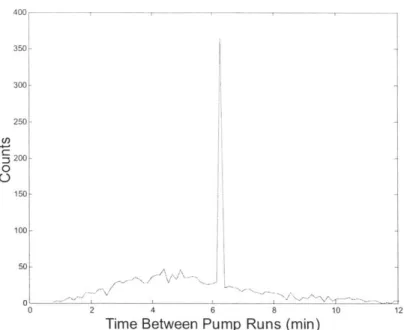
Time Between Pump Runs (min) Figure 3-14: Simulation with large leak

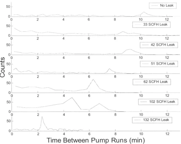
3.7 Field Tests

In order to correlate the cycling of the vacuum pumps with a fault (i.e. a leak) in the sewage system, vacuum leaks of various sizes were inserted into the sewage system onboard SENECA. The vacuum leaks were controlled using a MATHESON TRI-GAS flow meter attached to the vacuum collection tank gauge line. In order to introduce a leak, the throttle valve on the flow meter was adjusted to achieve the desired flow rate. At least 30 hours of inport data was collected for each of 7 different leak rates. Actual sewage leak data appears as shown in Figure 3-15.

Diagnostic indicators for shipboard systems using non-intrusive load monitoring

t*e

author heftby gmt

towM~

pSrT~sbn to

nd

to

disi~iute PUbliciy

,.>0peorld

elecwronIc copies

Of

t thei

document In whole or in part

~pameitfEletri

SEP 0

1

2005

Ie

AA KtER

j

Acknowledgements

Table of Contents

List of Figures

List of Tables

Chapter 1 Introduction

1.1

Motivation for Research

1.2 Increased Electrical Demand in Today's Naval Vessels

1.3

The NILM as a Monitoring Tool

1.4

Objective and Outline of Thesis

Chapter 2 Background

2.1

NILM Background

2.2

NILM Power Measurement on Electrical Systems

2.4

Improvements to the NILM System

# nilm5 reopened = 20041214-070002

for

i

in *.gz; do echo $i; gunzip -c $i > tempfile; grep -v

tempfile > ${i/.gz/.txt};done

Chapter 3 Cycling System Diagnostics

3.1

Introduction

3.2

SENECA Sewage System

0

3.3

Trend Analysis

3.4

Crew Flushing Patterns

50