Do housing sales drive prices or the converse?

Digitized

by

the

Internet

Archive

in

2011

with

funding

from

Boston

Library

Consortium

IVIember

Libraries

Ao.

08-oi

DEWEY

il

Massachusetts

Institute

of

Technology

Departnnent

of

Econonnics

Working

Paper

Series

DO

HOUSING

SALES DRIVE PRICES

OR

THE

CONVERSE?

William

C.

Wlieaton

Nai

Jia

Lee

Working

Paper

08-01

January

28,

2008

Room

E52-251

50

Memorial

Drive

Cambridge,

MA

02142

This

paper can be

downloaded

without

charge from

the

Social

Science

Research

Network

Paper

Collection at http;//ssrn.com/abstract=11

07525

HB31

Draft:January28, 2008.

Do

Housing

Sales

Drive

Housing

Prices

or

the

Converse?

By

William

C.

Wheaton

Department

of

Economics

CenterforRealEstate

MIT

Cambridge,

Mass 02139

wheaton@mit.edu

and

Nai

Jia

Lee

Department

of

Urban

Studies

and

Planning CenterforRealEstate

MIT

The

authorsare indebtedto,the

MIT

CenterforRealEstate, theNational Associationof

Realtors

and

toTorto

Wheaton

Research.

They

remain

responsiblefor allresults

and

conclusions derivedtherefrom.

ABSTRACT

Thisempiricalpaper

examines

the question

of whether

movements

inhousingsales

predict subsequent

movement

inhouseprices - ortheconverse.

The

former(positive)

relationship iswellhypothesized

by

severalfrictional search

models of

housing

market

transactions or

"chum".

The

latterrelationship has

been

hypothesized

by

two

theories.

Both

loss aversion

and

liquidity or

down-payment

constraints suggest anotherpositive relationship in

which

lowerprices generate lowersales

volume.

Our

contributiontothe

problem

of unraveling causalityis touse apanel

of

101 markets overthe period

from

1980

through 2006.

With

several differentestimation techniques

we

conclusivelyfind

thathighersales

volume

always generateshigher subsequentprices.

Higher

prices,

however

always generate

lower

subsequent sales volume.

Our

conclusionis thattheories

ofhousing loss aversionorfinancial

down

payment

constraintsjustare notconsistent

I. Introduction.

The

relationship

between

housingtransaction

volumes

{"sales")

and

price

movements

has

been

the subjectofseveral

economic models

-

with thedirectionof

causalitybeingquite different. In one

camp,

severalpapers in"behavioral

microeconomics" have

arguedthat

when

pricesfall,

homeowners

have

an aversion to

sellingata loss-

_no

matter

how

"rational" selling

may

be [Genesove and

Mayer

(2001),

Englehardt(2003)].

Another

group of papers

comes

to a similarconclusion,butthrough usingliquidity

and

down

payment

constraints

[Chan

(2001), Stein (1995),

Lamont

and

Stein (1999).

The

implication

of

both

micro-economic

theoriesisthat afterprice declines, salesshould

be

reduced,

and

followingpriceincreases, sales shouldrecover.

A

differentgroup ofpapers,

examine

how

owners

trade housinginthepresence of

search frictions

[Wheaton

(1990), Berkovic

and

Goodman

(1996),

Lundberg and

Skedinger(1999)].

As

istrue with

most

frictional

market

models

(e.g.Pissarides 2000), increasesinturnover(sales)tendsto

make

trading easier

and

inthe housing

market

this

will increaseprices.

Hence,

in this

camp

thehypothesisis thatpositive shocksto sales will thenincrease priceswhile negative shocks will depressthem.

There

have

been

onlya

few

attempts to test

whether

actual

movements

insales

and

pricessupport one, or the other,orboththeories

-

using timing asthe testof

causality. This is complicated

by

the factthatboththeoriespredict positiverelationships.

Berkovec and

Goodman

(1996) find

some

empirical supportforthe frictional

models

by

showing

that

demand

shocks first

show up

in sales

volume,

and

subsequentlyimpact

prices. Leung, Lau,

and

Leong

(2002) undertakea fulltime seriesanalysis

of

Hong Kong

Housing and

concludethatsimple

Granger

Causality is

found

more

oftenfor sales

drivingprices.

Andrew

and

Meen

(2003)

examines

thetimeseries forthe

UK

and

usinga

VAR

model, concludethattransactionsrespondto shocks

more

quicklythanprices,but

do

not

Granger Cause

price responses. Allofthese studiesare

hampered

by

shorttime

series

and

relatively

low

frequency.

Granger

tests are

known

to

more

valid

when

undertaken with

more

extensive observationsathighfi-equency.

Inthispaper,

we

trytosolve

some

ofthese

problems

with apanel approach

-

we

examine

the

movements

inprices

and

salesover

27

years(1980-2006) in 101

US

metropolitanareas.

With

almost

2500

observations

we

effectively ask

how

the

two

series

are related collectively acrossall

major

US

markets.

We

find strongevidencethat sales

positivelyimpact subsequentprices,butthatpricesnegativelyimpact subsequentsales.

We

obtain theseresultswith FixedEffects estimation

and

alsowith

GLS

IV

estimates

thatcorrectforthepanelHeteroskedasticityidentified

by

Holtz-Eakin,

Newey

and

Rosen

(1988). Furthermore, ourresults arerobustto

whether

the

models

are estimatedin levels

(whichare

non

stationary)orinfirst-differences

(which

arestationary).

We

concludethat

theoriesof

Loss Aversion and

Liquidity constraints arejustnotconsistentwiththe

aggregatebehavior

of

US

housingdata,whilethere iscomplete consistency with

frictionaltradingmodels.

Our

paperis organizedas follows. In sectionII

we

reviewthe varioustheoretical

arguments

and

empirical supportforthe

two

typesofrelationships

between

sales

volume

and

housingprice

movements.

In sectionIII,

we

reviewthedatasources

and

find

some

interesting

and

yetpuzzlingtrends intheonly availabletimeseries forsales.

These

trends

generatenon-stationarity

and

encourage estimation indifferences. In section

IV

we

discuss the applicationof panel datatoourquestion, theuseof conditioning variables

and

thealternativeestimationapproaches, whilein section

V

we

discuss the resultsof each

specification. Section

VI

illustrates

how

our equations operatetogether as a

VAR

model

and

Section

VI

draws

some

conclusions as to

why we

getaggregateresults thatare so

different fi^omthemicro-level research.

IL

Sales

Volume-

Price relationshipsin the Literature.

There

are aseriesofpaper's

which

propose a relationshipin

which

prices or

changes inprices will subsequently "cause"sales

volumes

to adjust.

The

firstofthese is

by

Stein (1995) followed

by Lamont

and

Stein (1999)

and

then

Chan

(2001). In these

models,liquidity constrained

consumers

aremostly

moving

from one house

to another (market

"chum")

and

must

make

a

down

payment

inordertopurchase housing.

Wlien

prices decline

consumer

equitydoes likewise

and

fewer households

have

theremaining

down

payment

to

make

thelateral

move.

As

pricesrise, equityrecovers

and

sodoes

market

liquidity. Ineffectprice changes shouldpositivelycausesales

volumes

-

both

up

and

down

-

althoughnot necessarilywith

symmetry.

A

second series of papers suggestadifferent

mechanism

which

also generatesat

leastapartialpositive causal chain

between

prices

and

salesvolume. Relying

on

"behavior economics",

Genesove and

Mayer

(2001)

and

thenEnglehardt (2003)testfor

whether

sellers

who

will experiencealoss

when

theyselltendto sethigherreservations

thanthose

who

willnotexperiencealoss. This suggests that aspricesbegintodrop,only

recentbuyerswill experience such "loss aversion".

As

aperiod ofpricedeclines extends,

however,

an ever greater

number

of

buyers experience "lossaversion"

and

withthis

transaction

volume

willincreasinglydry

up

as

more

and

more

potentialsellers setoverly high

and

unattainable reservations.

As

long asprices arerising,

however,

thetheory

makes

littleprediction about

what

will

happen

to sales

volume

otherthaneliminating the

source of

any

"loss aversion".

The

theory alsodoes notaddress the equilibriumquestion of

what

eventually

happens

toprices ifallpotential sellers

have

higherreservations.

Do

prices stopfalling for

example?

A

different group ofpapers,explicitly

models

how

owners

tradehousingin the

presence ofsearch frictions

[Wheaton

(1990),

Lundberg and

Skedinger(1999)]. In these

models, buyers

must

always

become

sellers

-

there are

no

entrantsorexits

from

the

market. Insuch a situationprices arelike "ftinny

money" -

withparticipantspaying

more

butalsoreceivingmore. It isonly thetransaction costof

owning

2

homes

(during the

moving/tradeperiod) that groundsprices. Ifpricesare high, thetransaction costs can

make

moving

soexpensive as toerase

whatever

gains

from

moving

were

there originally.

Inthis

environment

Nash-bargainedprices

become

almostinverse toexpectedsales times -

_where

_thelatterequals

vacancy

divided

by

the sales flow. Inthese models,

vacancy

is

exogenous, butsales flowis

endogenous

-

depending

inpart

on

an

exogenous

rate of

"chum".

As

long as anincrease inthe

"chum

rate"does not reduce searcheffort, sales

timewill

be

shorterwith

more

chiom

and

pricestherefore higher. In a similarmanner,

and

followingPissarides (2000),

Berkovec and

Goodman

(1996) developa

model

in

which

a

reduction (increase) insales

volume

generatesa greater (smaller) inventory

of

unsold

homes, and

this in

tum

leadsto

lower

(higher) sellerreservations. Inbothofthese

models,there is cleartemporal causality: a

shock

occurs firstto sales

volume

which

then

There have been few

attemptsto test

whether

actual

movements

insales

and

prices supportone, or theother, orboththeories. This is complicated

by

the fact thatboth

theories predict positiverelationships,justwithdifferent timing. Berkovic

and

Goodman

(1996)initiallyfoundthat

movements

in

volume

did lead

movements

inprices

and

inferredthat this

was

consistentwiththeirtheory. Leung, Lau,

and

Leong

(2002) undertake atime series analysisof

Hong Kong

Housing and

concludethatstronger

Granger

Causality is foundfor sales driving prices ratherthanpricesdrivingsales.

Andrew

and

Meen

(2003)

examines

atime seriesforthe

UK

and

usinga

VAR

model, conclude thattransactionsrespond toshocks

more

quickly thanprices,but

do

not necessarily

"Granger

Cause"

price responses. Intheir

VAR

model

itturnsoutthatthe

estimated coefficientof laggedprices

on

transactions

volume

isnegative

and

notpositive

as suggested

by

thetheoriesofloss aversion orliquidityconstraints.

III. Sales

Volume

and

Price Data.

The

price data

we

chose touseis the

OFHEO

repeatsales series [Baily,

Muth,

Nourse

(1963)]. This data serieshasrecently

been

severely questionedfornotfactoring out

home

improvements

or

maintenance and

fornotfactoring indepreciation or

obsolescence [Case,

PoUakowski,

Wachter

(1991),Harding, Rosenthal,

Sirmans

(2007)].

These

omissions couldgenerate a significantlybias inthe long termtrend

of

the

OFEHO

series. Thatsaid

we

areleftwith

what

isavailable,

and

the

OFHEO

index is the

most

consistentseries availablefor

most

US

markets overalong timeperiod.

The

only

alternative istopurchase similarindices

from

CSW/FISERV,

although they

have

the

same

methodologicalissues as the

OFHEO

data.

The

sales data

we

use

were

provided

by

theNational Association

of

Realtors

(NAR).

This datais for singlefamilyunitsonly (it excludes

condominium

sales), and

was

obtainedforeach

market

from

1980-2006.

Raw

sales

were

then

compared

with annual

Census

estimates ofthe

number

oftotalhouseholds inthose markets. Dividingsingle

familysales

by

totalhouseholds

we

getacrudesales rate foreach market. In

1980

this

sales ratevaried

between

1.2%

and

5.1%

across ourmarkets with an average of 2.8%.

By

contrast, inthe

1980

Census,the single family mobilityrate(inthe previousyear)

(1989)

Census

annual mobility ratefellto 6.5%.

By

2000,the

NAR

sales ratereached 5.0%, whilethe

Census

mobilityraterecoveredabitto7.1%).

Thus

duringthis25 year

period, ourcalculatedaverage sales ratesarealways lower thanthe censusreported

mobilityrates. This isbecausethe householdseriesusedtocreatetherate is total

householdsratherthanjust singlefamily

owner-occupied

households. Separate

renter/ownersinglefamily

household

series atyearly

frequency

arejustnot available

by

metropolitanmarket.'

However,

the observationthatthe

two

datasources trend

differentlyis

more

disturbing.

Over

1980-2000, boththe

US

homeownership

ratio

and

the

fraction ofsingle familyunits in thestock are virtuallyunchanged.

As

such, the

difference

between

thetrue mobility

and

ourconstructedsale rate should

be

constant. It is not,

and

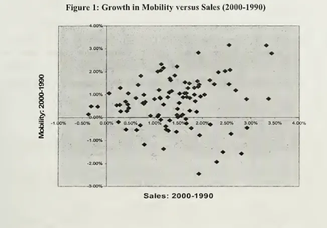
inFigure 1

we

show

ascatterplot that illustratesthe relationship

between

the

changes

inthese

two measures

across our 101 markets.

The

NAR

sales rateincreases

significantly

between

1

990 and

2000

in

most

MSA,

whilethe

Census

mobilityrate

decreases inalmostas

many

areas as itincreases. Itis clearthatthere is

no

association

overthis

decade

between

which

markets

saw

an increasein

NAR

sales

and

which

experienced

any

underlying increase in

Census

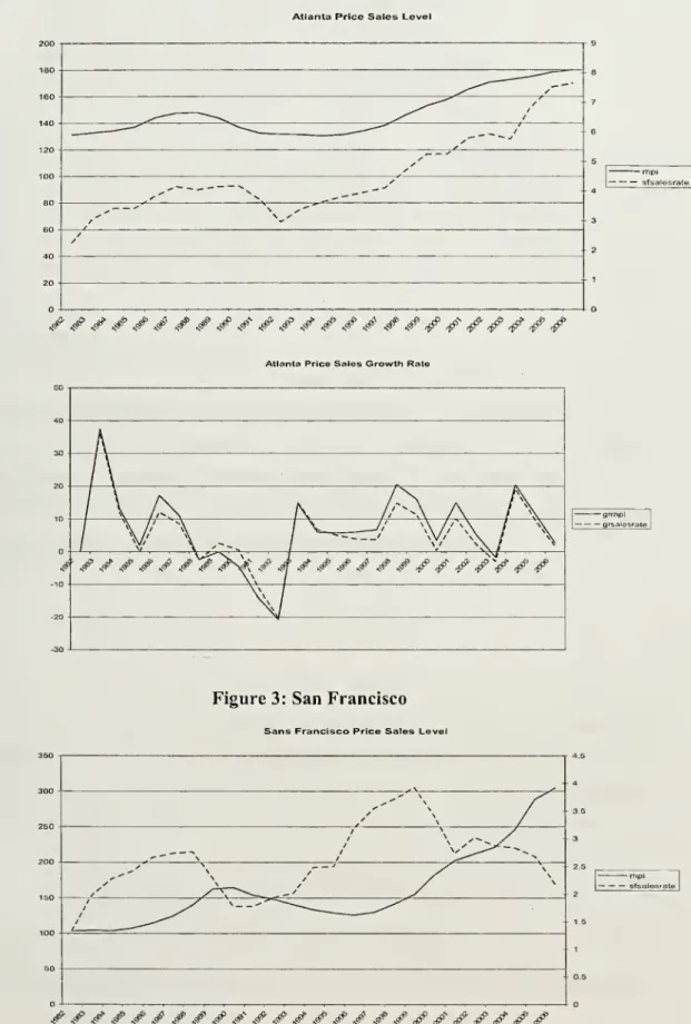
mobility(R~=.002).

InFigures2

and

3

we

illustratetheyearly

NAR

sales rate data, along with the

constant dollar

OFHEO

price series

-

bothin levels

and

differences for

two

marketsthat

exhibit quitevaried behavior, Atlanta

and San

Francisco.

Over

thistime frame, Atlanta's constant dollar prices increaseverylittlewhile

San

Francisco's increasedalmost200%).

San

Francisco prices,

however,

exhibit fargreaterpricevolatility. Atlanta'saverage sales rateis closeto

5%

and

trends quite sharply,while

San

Francisco's is almosthalfofthat

(2.6%))

and

exhibits onlya slight trend.

'

Inmorerecent years the calculated

NAR

sales ratesare closetobeing

60%

ofthetruesinglefamily

mobilityrate-aswouldbedictatedbythe national differencebetweenthenumberoftotalandsingle

Figure

1:

Growth

in Mobility versus Sales(2000-1990) CM 1.00% ^.00% 1,00% -0.50% O.OO'

/i.

%

—

-

—

^

>

^

'

—

^ • ' • % 0.50%^ 1.00% ^^1.50°/* 2.00°/,^ 2.50% 3.00% 3.50% 4.'

^*

Sales:

2000-1990

Both

ofthese individualmarketsillustrate thetrendtothe sales ratedatathatis *

presentin virtuallyall

MSA.

The

constructedsales ratesalvv^aysrise

upwards

overthis 25 year period

-

sometimes

increasingcumulatively

by

as

much

as 2to

4

percentagepoints.

As

mentioned

relative to Figure 1,the

Census

reportsonly aslightincrease inboth

owner

and

renter

"move"

rates

between 1990 and

2000 and

adecline

between 1980 and

1990.

Thus

the

NAR

trend

would

appeartorepresent

some

artifactofreporting. Perhaps a

growing

shareof brokers

became

members

ofthe

NAR

or a

growing

share of

members

participatedinreportingdata.

Whatever

thereason,it

seems

clearthatthetrenddoes not

reflect a truedoubling in

US

mobility. Itisdifficulttothinkof reasons

why

sales

would

trend significantly different

from

mobility

-

particularly acrossmarkets^. InappendixI

we

present the

summary

statistics foreach market'sprice

and

sales rateseries.

Given

thereservations overthetrends inbothseries itisuseful

and

important to

testfor series stationarity.

There

are

two

testsavailable forusewith panel datasuchas

we

Salesduetodeathsdonot generateamove.Transfersof propertybetweenindividualscouldgeneratea

"sale"withoutamove. Thesebiasesshouldbesmallandstationaryhowever. Itis also believedthat For-Sale-by-Owner"transactionshaveincreasedanderoded brokerage businessrecently-the oppositeofthe

have. In each, thenullhypothesis is that allofthe individualseries

have

unitroots

and

are

non

stationary. Levin-Lin (1993)

and

Im-Persaran-Shin (2002) both developatest

statistic forthe

sum

oraverage coefficientofthe laggedvariable

of

interest

-

across the individuals (markets) within the panel.

The

nullis thatall or the average ofthese coefficients isnotsignificantly different

from

unity. InTable 1

we

report the results

of

thistestforbothhousingprice

and

sale rate levels,aswellas a 2" orderstationarity test forhousingprice

and

sales ratechanges.

TABLE

1

RHPI

(Augmented

bv

1 lag)

Levin

Lin's

Test

Coefficient

T

Value

T-Star

P>T

Levels -0.10771 -18.535

0.22227

0.5879

First Difference -0.31882 -19.822 -0.76888 0.2210

IPS

test

T-Bar

W(t-bar)

P>T

Levels -1.679 -1.784 0.037

FirstDifference -1.896 -4.133 0.000

SFSALESRATE

(Augmented

by

1 lag)

Levin

Lin's

Test

Coefficient

T

Value

T-Star

P>T

Levels -0.15463 -12.993 0.44501 0.6718

FirstDifference -0.92284 -30.548 -7.14975 0.0000

IPS

test

T-Bar

W(t-bar)

P>T

Levels -1.382 1.426 0.923

FirstDifference -2.934 -15.377 0.000

With

the Levin-Lintest

we

cannotreject thenull (non-stationarity) for either

house

pricelevels ordifferences. Interms ofthesales,

we

canrejectthe null for

differencesin sales ratedifferences, butnotfor levels.

The

IPS test

(which

isarguedto

have

more

power)

rejects thenull for

house

price levelsand differences

and

for sales rate

differences. In short,bothvariables

would seem

to

be

stationary indifferences,butlevels are

more

problematic

and

likely non-stationary.

Figure

2:

Atlanta

AtlantaPriceSales Level

* _sfsalesrate

^ ^

.^ ^#

^

/

^

.^

^

^^

^ ^

^

^

_.#

,^\^.^^^^^^^^^

AtlantaPriceSalesGrowthRate

Figure

3:

San

Francisco

SansFrancisco Price Sales Level

-rtipl

'sfsalesrate

SansFranciscoPricesSalesGrowth

IV.

Panel Estimation

Approaches.

Our

panelapproachuses a

well-known

application of Granger-lypeanalysis.

We

will ask

how

significantlagged salesareinapanel

model

ofprices

which

uses lagged

prices

and

thenseveral conditioning variables.

The

conditioning variables

we

choose are

market

area

employment,

and

national

mortgage

rates.

The

companion

model

isto ask

how

significant laggedprices are inapanel

model

ofsalesusinglagged sales

and

the

same

conditioningvariables. This pairof

model

is

shown

(l)-(2).

P,j

= ^0 +

«i-^-,r-i

+

«2'5'/,r-i

+ P'Xfj

+

^,

+

£,j (1)

s^j

=

_ro

+

y^s,,T-^

+

riPi.T-i

+ ^'^ij +

+7,-

+

^,, (2)

Inpanel models, all ofthe estimation issues raisedintime series continueto exist. Inourcase thereisconcern about the stationarityof bothprice

and

sales rate levels. This

same

concernis notpresentfordifferences.

Hence

clearly

we

will

need

to estimate the

model

in firstdifferencesas wellaslevels

-

as

outUned

inequafions (3)

and

(4).''

AP.j

=

«(,

+

a^AP.j._^

+

a2AS.j._^

+

fi'AX-j.

+

+S,

+

_£,j (3)

A5,,r

=n+

rAS,,T-^

+ Yi^.j-x +

^'^X.j

+

+TJ.

+

£,., (4)

Inpanel

models

with a cross-section fixedeffect(theS.

and

rj.) there exists a

potential specification issue. Sincethe fixedeffectsare presentnotjust in current, but laggedvalues ofthe

dependent

variables,

OLS

willnot leadtoconsistent estimates.

The

problem

isabuilt in correlation

between

the laggeddependentvariable

and

the lagged

error term.

Thus

estimates

and

tests

on

theparameters ofinterest (the

a

and

_/

)

may

not be

reliable.

The

problem

can

be

amelioratedto

some

extent

by

normalizing thevariablesto

make

the fixedeffectsvanish -for

example

when

prices are

measured

asan index that

begins with avalueof 100 for each cross sectioninthesample. Similarlyusingasales

rate(ratherthan theactual sales

volume)

willhelp alleviate the specificationproblem.

To

be

safe,

however,

we

also estimatedthe

models

followingan estimation strategy

by

Holtz-Eakin et altobetter estimate the causalvalues oftheparametersofinterest.

As

discussedin

Appendix

II,this

amounts

tousing 2-periodlaggedvaluesofsales

and

prices as instrumentswith

GLS

estimation.

From

eitherestimates,

we

conducta

"Granger"

causalitytest. Since

we

areonly

testing for a singlerestriction, the/statistic isthe squarerootofthe

F

statistic that

would

be

used

to testthe hypothesisinthepresenceofa longer lagstructure (Green, 2003).

Hence,

we

can simply use attest(appliedtothea,

and

y^)as thecheck of

whether

changes

in sales

"Granger

cause" changes inprice and viceversa.

V. Results.

Intable 2

we

report theresults ofequations(1) through(4) ineachsetof rows.

The

first

column

uses

OLS

estimation, the second the

Random

Effects

IV

estimates

from

Holtz-Eakinetal.

The

first setof equationsis in levels, whilethe second set

of

rows

reports theresultsusingdifferences.

Among

the levels equations,

we

firstnoticethatthe

two

conditioningvariables,

thenational

mortgage

rate

and

local

employment

can

have

the

wrong

signs

-

here in

two

cases.

The

mortgage

interestrateinthe

OLS

pricelevelsequation

and

local

employment

inthe

IV

sales rateequation aremiss-signed.Thereis alsoan insignificant

employment

troublesomeresultisthatthepricelevelsequationhas excess

"momentum" -

lagged

prices

have

a coefficient greater than one.

Hence

prices(levels)

might

grow

on

their

ovm

withoutnecessitating

any

increases infundamentals, orsales.

We

suspectthatthese

two

anomalies arelikelythe resultofthenon-stationary featuretoboththe price

and

sales

series

when

measured

in levels. Interestingly,the

two

estimationtechniquesyield quite

similarcoefficients

-

as wellas anomalies.

When we

move

totheresults

of

estimating theequationsindifferences these

issues alldisappear.

The

laggedpricecoefficients are small, the price equations stable in

the 2"^degree,

and

the signs ofallcoefficients are both correct

-

and

highly significant.

As

to the questionofcausality, inevery price or price

growth

equation, lagged

sales or

growth

in salesis always significant.Furthermorein everysales rate or

growth

in

sales rateequation, laggedprices(orits growth)arealsoalways significant.

Hence

there

isclear evidenceofjoint causality, butthe effect

of lagged

prices

on

sales isalways

_of

the

wrong

sign!

Holding

lagged sales(andconditioning variables) constant, ayear after

thereis

an

increase inprices

-

salesfall

-

ratherthanrise!

The

impactis exactly the opposite ofthatpredicted

by

theoriesoflossaversionorliquidityconstraints.

TABLE

2

FixedEffects

E

Holtz-Eakinestimator Levels

RHPI

(Dependent

Variable) Constant

RHPI

(lag 1)

SFSALESRATE(lagl)

MTG

EMP

SFSALESRATE

(Dependent

Variable) Constant

RHPI

(lag 1)

SFSALESRATE

(lag 1) -25.59144" (2.562678) 1.023952** (0.076349) 3.33305** (0.2141172) 0.3487804** (0.1252293) 0.0113145** (0.0018579) 2.193724** (0.1428421) -0.0063598** (0.0004256) 0.8585273** -12.47741** (2.099341) 1.040663** (0.0076326) 2.738264** (0.2015346) -0.3248508** (0.1209959) 0.0015689** (0.0003129) 1.796734** (0,1044475) -0.0059454** (0.0004206) 0.9370184**

(0.0119348) (0.0080215)

MTG

-0.063598** -0.0664741** (0.0069802) (0.0062413)

EMP

-0.0000042 -0.0000217** (0.0001036) (0.0000103) FirstDifference

GRRHPI

(DependentVariable) Constant -0.4090542** -0.49122** (0.1213855) (0.1221363)

GRRHPI

(Lag 1) 0.7606135** 0.8008682** (0.0144198) (0.0148136)

GRSFSALESRATE

0.0289388** 0.1826539** (Lag1) (0.0057409) (0.022255)

GRMTG

-0.093676** -0.08788** (0.097905) (0.0102427)

GREMP

0.3217936** 0.1190925** (0.0385593) (0.048072)

GRSFSALESRATE

(DependentVariable) Constant 0.7075247 1.424424** (0.3886531) (0.3710454)

GRRHPI(Lagl)

-0.7027333** -0.8581478** (0.0461695) (0.0556805)

GRSFSALESRATE

0.0580555** 0.0657317** (Lagi) (0.0183812) (0.02199095)

GRMTG

-0.334504** -0.307883** (0.0313474) (0.0312106)

GREMP

1.167302** 1.018177** (0.1244199) (0.1120497) ** _{indicates significance at}

_5%.

We

have

experimented withthese

models

using

more

than a singlelag,but

qualitativelytheresults arethesame. Inlevels, the priceequationwith

two

lags

becomes

dynamically stable inthe sense thatthe

sum

ofthe laggedprice coefficientsislessthan

one.

As

to causal inference, the

sum

ofthe laggedsales coefficients ispositive,highly

significant,

and

passes the

Granger

F

test. In thesales rateequation, the

sum

ofthe

two

laggedsales rates is virtually identical tothe single coefficient

above

and

the laggedprice

levels areagain significantlynegative (intheir

sum) and

collectively

"Granger

cause" a

reduction in sales.

We

have

similarconclusions

when

two

lags are

used

inthe differences equations, butindifferences, the2" lagis always insignificant.

As

a finaltest,

we

investigatea relationship

between

the

growth

in

house

prices

and

the levelofthe salesrate. In the search theoretic

models

sales ratesdetermine price

levels,butifprices are

slow

to adjust, the impactofsales

might

better

show

up on

price

changes. Similarly the theories oflossaversion

and

liquidity constraintsrelateprice

changesto sales levels.

While

the

mixing of

levels

and

changes in timeseries analysisis

generally not standard,

we

offer

up

Table 3

where

price

changes

are tested against the

levelofsales (as arate).

TABLE

3

Differences

and

Levels Fixed Effects

_E

_Holtz-Eakinestimator

GRRHPI

(Dependent

Variable) Constant

GRRHPI

(lag 1)

SFSALESRATE

(lag 1)

GRMTG

GREMP

SFSALESRATE

(Dependent

Variable) Constant

GRRHPI

(lag 1)

SFSALESRATE

(lag 1)

GRMTG

-6.61475** (0.3452743) 0.5999102** (0.0155003) 1.402352** (0.0736645) -0.1267573** (0.0092715) 0.5059503** (0.0343458) -0.0348229 (0.0538078) -0.0334235** (0.0024156) 1.011515** (0.0114799) -0.0162011** (0.0014449) -1.431187** (0.2550279) 0.749431** (0.0141281) 0.2721678** (0.0547548) -0.0860948** (0.0095884) 0.3678023** (0.0332065) 0.0358686 (0.0026831) -0.0370619** (0.0026831) 1.000989** (0.0079533) -0.0151343** (0.0014294)

GREMP

0.0494462** (0.0053525) 0.043442** (0.0049388) ** _{indicates significance at}

_5%

Interms ofcausality, theseresults are

no

differentthanthe traditional

models

estimated

either in all levelsorall differences.

One

yearafteranincrease inthe levelofsales,the

accelerates thelevel

of

home

sales falls(ratherthanrises). All conditioning variables are

significant

and

correctlysigned

and

lagged

dependent

variables

have

coefficientless than

one.

VI.

VAR

System

Behavior.

The

final step in our analysis is to investigate the

dynamic

relationship

between

the

two

variables: sales

and

prices.

When

taken together, they represent a 2-equation

Vector

Auto

Regression

(VAR).

VARs

are

most

useful for understanding the long-term response ofa system of equations to a

shock

or

change

in a conditioning variable.

Thus

for

example what happens

to prices

and

sales if

mortgage

rates

permanently

decrease or

employment

permanently increases? In Figure 4

we

examine what happens

to in a

representative

market

(Atlanta in this case)

when

mortgage

rates take a

permanent

drop.

The model

uses the levels equations

and

the base line steady state

assumes

that current

Atlanta

employment

levels

and

mortgage

rates prevail indefinitely. This generates a

steady state price index of

273 and

sales rate of 1.24%.''

When

rates permanently drop

200

bps sales initially rise but then settle

down

just slightly

above

their original value.

Prices rise

10%

butfollow the

movement

in sales.

Both

ofthese response patterns

seem

in accord with theory

and

suggest that

when

taken together the levels equations closely

reflect

how

housing markets shouldreactto

demand

shocks.

In Figure 5

we

examine

the behavior

of

the pair of equations estimated in

differences.

Here

our base line steady

growth

path has Atlanta

employment

increasing

2%

yearlywhile

mortgage

rates are stable.

The

impulse responsetracesout

what happens

ifthe

employment

growth

rate permanently

jumps

to a very robust

4%.

Prices,

which

were

trendingat

0.057%,

now

grow

at a little

more

than

5.53%

while the sales rate

jumps

from

2.27%

to

3.15%

at steady state. In impulse responses there is the appearance that

sales

move

"before"prices.

Thesimulations reported incorporate the fixedeffectfor the Atlantamarket,whichlike that formost

marketswasnotstatistically significant.

We

attribute thistotheuseofsalesratesandtoprice indices

Figure

4:

ChangeinMortgage Rate by 200 bps

Quarters

-rhpi

sfsalesrale

Figure

5:

NewSteadyStates:IncreaseinEmployment GrowthRateby4%

o 6 0. 2 -gntipi -grsfsalesrate 1 2 3 4 5 6 7 8 9 101 112 13 14 15 16 17 18 192021 22 23 24 25 26 27 28 29 3031 32 33 34 3536 Quarters

VI. Discussion

and

Extension.

On

the

one

hand, theresults

of

thisanalysis arecompletelyconsistentwith

theories

of

frictionalmarketsin

which

changesto housingsales should

"Granger

cause" housingpricesto increase.

On

theother

hand

theyarecompletelyinconsistentwith

theoriesoflossaversion or liquidity constraints,

wherein

falling (rising)

house

prices

shouldconstrain(free up)buyers

and "Granger

cause"sales to fall(rise). Instead, sales inthe

market

tendtoreactnegatively topriorprice

movements.

This occurs in

models

of bothprice levels aswellas differences

and

is alwaysstatisticallysignificant.

As

to

why

we

getthisresult,here

we

offer

some

possible explanations.

First,with the increased sophisticationof

mortgage

marketsinthe last

two

decades,

down

payment

constraints

may

have

been

reducedtothepoint

where

theyrarely

exercise influence

on

home

buying.

Secondly, duringaperiod

when

nominal house

pricesrose almost every yearin

most

markets,thepresence

of

lossaversion

may

likewiseexistonlyina

few

markets

and

during onlya

few

periods.

Such

episodesare simplytoo infrequentto impactthe

market

as a

whole even though

theycan

show

up

in individual decisions.

Finally,itcould bethe casethattheaggregate

movement

in housingsales is

largelydriven

by

flows into

home-ownership.

If infact, firsttime

home

buyers arean important source ofsalesfluctuations, thenitis nothardto understand

how

such purchasesarenegatively correlatedwithprices.

As

prices rise(fall) fewer (more)first

timebuyersare abletoafford

and

enter the

ownership

market. This isprobably ourbest

explanationfor

why

ourresultsusingaggregatedatastandinsuchcontrasttothe

REFERENCES

Andrew,

M.

and

Meen,

G. (2003).

"House

price appreciation, transactions

and

structural

change

inthe Britishhousing market:

A

macroeconomic

perspective."

Real

Estate

Economics,

31, 99-116.

M.J. Baily, R.F.

Muth, H.O.

Nourse,

"A

Regression

Method

forReal Estate Price

Index

Constmction"

,Journal

of

the

American

StatisticalAssociation, 58 (1963) 933-942.

Berkovec, J.A.

and

Goodman,

J.L. Jr. (1996).

"Turnover

as a

Measure of

Demand

for

Existing

Homes."

Real

Estate

Economics,

24(4),421-440.

Bradford Case,

Henry

O. Pollakow^ski,

and Susan

M.

Wachter.

"On

Choosing

among

Housing

PriceIndexMethodologies,"^i?£'t/^^ Journal, 19 (1991), 286-307.

Dennis

Capozza, PatricHendershott,

and

Charlotte

Mack.

"An Anatomy

ofPrice

Dynamics

in IlliquidMarkets: Analysis

and Evidence

from

Local

Housing

Markets,"

Real

Estate

Economics,

32 (2004) 1-21.

Chan,

S. (2001). "SpatialLock-in:

Do

Falling

House

Prices ConstrainResidential

Mobility?"

Journal of

Urban

Economics,

49,567-587.

Engelhardt,G. V. (2003).

"Nominal

lossaversion,housing equityconstraints,

and

household

mobility: evidence

from

theUnited States."

Journal of

Urban

Economics,

53(1), 171-195.

Genesove,

D.

and

C.

Mayer

(2001). "Lossaversion

and

sellerbehavior:

Evidence from

the

housing

market." Quarterly

Journal ofEconomics,

116(4), 1233-1260.

John

Harding, S. Rosenthal, C.F.Sirmans. (2007). "Depreciation of

Housing

Capital,

maintenance,

and house

priceinflation..

."

Journal of

Urban

Economics,

61,2,567-587.

Holtz-Eakin, D. ,

Newey,

W.

and

Rosen, S.H. (1988). "EstimatingVector

Autoregressions with Panel Data," Econometrica,Vol. 56,

No.

6. _pp. 1371-1395.

Kyung

So

Im,

M.H.

Pesaran, Y. Shin(2002),"Testing forUnit

Roots

in

Heterogeneous

Panels",

Cambridge

University,

Department of

Economics

Lament,

O.

and

Stein, J. (1999).

"Leverage and

House

Price

Dynamics

inU.S. Cities."

RAND

Journal ofEconomics,

30, 498-514.

Levin,

Andrew

and

Chien-Fu

Lin (1993). "Unit

Root

Tests inPanel Data:

new

results."

Discussion

Paper

No. 93-56,

Department of Economics,

UniversityofCaliforniaat

San

Leung,

C.K.Y.,Lau,

G.C.K. and

Leong, Y.C.F. (2002). "Testing AlternativeTheories of

the Property Price-Trading

Volume

Correlation."

The

Journal

_{of Real}

EstateResearch,

23(3), 253-263.

Per Lundborg, Per Skedinger, "Transaction

Taxes

ina Search

Model

ofthe

Housing

Market", Journal

of

Urban

Economics,

45,2,

March

1999.

Pissarides, Christopher,Equilibrium

Unemployment

Theory,2" edition,

MIT

Press,

Cambridge,

Mass., (2000).

Seslen,T.N. (2003).

"Housing

Price

Dynamics

and

Household

Mobility Decisions."

Working

Paper,

The

CentreforRealEstate,M.I.T.

Stein, C. J. (1995). "Prices

and

Trading

Volume

inthe

Housing

Market:

A

Model

with

Down-Payment

Effects,"

The

Quarterly

Journal

Of

Economics,

110(2), 379-406.

Wheaton,

W.C.

(1990).

"Vacancy,

Search,

and

Prices in a

Housing

Market

Matching ModeX," Journal of

Political

Economy,

98,

1270-1292

APPRENDIX

I Market

Code

Market Average

GRRHPI

{%) Average

GREMP

(%) Average

SFSALES

RATE

Average

GRSALES

RATE

(%) 1 Allentown 2.03 1.10 4.55 4.25 2 Akron 1.41 1.28 4.79 4.96 3 Albuquerque 0.59 2.79 5.86 7.82 4 Atlanta 1.22 3.18 4.31 5.47 5 Austin 0.65 4.23 4.36 4.86 6 Bakersfield 0.68 1.91 5.40 3.53 7 Baltimore 2.54 1.38 3.55 4.27 8 Baton

Rouge

-0.73 1.77 3.73 5.26 9

Beaumont

-1.03 0.20 2.75 4.76 10 Bellingham 2.81 3.68 3.71 8.74 11 Birmingham 1.28 1.61 4.02 5.53 12 Boulder 2.43 2.54 5.23 3.45 13 BoiseCity 0.76 3.93 5.23 6.88 14 Boston

MA

5.02 0.95 2.68 4.12 15 Buffalo 1.18 0.71 3.79 2.71 16 Canton 1.02 0.79 4.20 4.07 17 Chicago IL 2.54 1.29 4.02 6.38 18 Charleston 1.22 2.74 3.34 6.89 19 Charlotte 1.10 3.02 3.68 5.56 20 Cincinnati 1.09 1.91 4.87 4.49 21 Cleveland 1.37 0.77 3.90 4.79 22

Columbus

1.19 2.15 5.66 4.61 23 Corpus Christi -1.15 0.71 3.42 3.88 24 Columbia 0.80 2.24 3.22 5.99 25 Colorado Springs 1.20 3.37 5.38 5.50 26 Dallas-Fort Worth-Arlington -0.70 2.49 4.26 4.64 27 Dayton

OH

1.18 0.99 4.21 4.40 28 Daytona Beach 1.86 3.06 4.77 5.59 29 Denver

CO

1.61 1.96 4.07 5.81 30

Des

Moines 1.18 2.23 6.11 5.64 31 DetroitMl 2.45 1.42 4.16 3.76 32 Flint 1.70 0.06 4.14 3.35 33 Fort Collins 2.32 3.63 5.82 6.72 34 Fresno

CA

1.35 2.04 4.69 6.08 35 Fort

Wayne

0.06 1.76 4.16 7.73 36 Grand Rapids Ml 1.59 2.49 5.21 1.09 37 Greensboro

NC

0.96 1.92 2.95 7.22

38 Harrisburg

PA

0.56 1.69 4.24 3.45 39 Honolulu 3.05 1.28 2.99 12.66 40 Houston -1.27 1.38 3.95 4.53 41 Indianapolis IN 0.82 2.58 4.37 6.17 42 Jacksonville 1.42 2.96 4.60 7.23 43 KansasCity 0.70 1.66 5.35 5.17 44 Lansing 1.38 1.24 4.45 1.37 45 Lexington 0.67 2.43 6.23 3.25 46 Los Angeles

CA

3.51 0.99 2.26 5.40 47 Louisville 1.48 1.87 4.65 4.53 48 Little

Rock

0.21 2.22 4.64 4.63 49 Las

Vegas

1.07 6.11 5.11 8.14 50

Memphis

0.46 2.51 4.63 5.75 51 Miami FL 1.98 2.93 3.21 6.94 52 Milwaukee 1.90 1.24 2.42 5.16 53 Minneapolis 2.16 2.20 4.39 4.35 54 Modesto 2.81 2.76 5.54 7.04 55

Napa

4.63 3.27 4.35 5.32 56 Nashville 1.31 2.78 4.44 6.38 57

New

York 4.61 0.72 2.34 1.96 58

New

Orleans 0.06 0.52 2.94 4.80 59

Ogden

0.67 3.25 4.22 6.08 60

Oklahoma

City -1.21 0.95 5.17 3.66 61

Omaha

0.65 2.03 4.99 4.35 62 Orlando 0.88 5.21 5.30 6.33 63 Ventura 3.95 2.61 4.19 5.83 64 Peoria 0.38 1.16 4.31 6.93 65 Philadelphia

PA

2.78 1.18 3.52 2.57 66 Phoenix 1.05 4.41 4.27 7.49 67 Pittsburgh 1.18 0.69 2.86 2.75 68 Portland 2.52 2.61 4.17 7.05 69 Providence 4.82 0.96 2.83 4.71 70 PortSt. Lucie 1.63 3.59 5.60 7.18 71 Raleigh

NC

1.15 3.91 4.06 5.42 72

Reno

1.55 2.94 3.94 8.60 73

Richmond

1.31 2.04 4.71 3.60 74 Riverside 2.46 4.55 6.29 5.80 75 Rochester 0.61 0.80 5.16 1.01 76 Santa

Rosa

4.19 3.06 4.90 2.80 77 Sacramento 3.02 3.32 5.51 4.94 78

San

Francisco

CA

4.23 1.09 2.61 4.73

79 Salinas 4.81 1.55 3.95 5.47 80

San

Antonio -1.03 2.45 3.70 5.52 81 Sarasota 2.29 4.25 4.69 7.30 82 Santa Barbara 4.29 1.42 3.16 4.27 83 SantaCruz 4.34 2.60 3.19 3.24 84

San

Diego 4.13 2.96 3.62 5.45 85 Seattle 2.97 2.65 2.95 8.10 86

San

Jose 4.34 1.20 2.85 4.55

87 SaltLake City 1.39 3.12 3.45 5.72

88 St. Louis 1.48 1.40 4.55 4.82

89

San

Luis Obispo 4.18 3.32 5.49 4.27

90

Spokane

1.52 2.28 2.81 9.04 91 Stamford 3.64 0.60 3.14 4.80 92 Stockton 2.91 2.42 5.59 5.99 93

Tampa

1.45 3.48 3.64 5.61 94 Toledo 0.65 1.18 4.18 5.18 95 Tucson 1.50 2.96 3.32 8.03 96 Tulsa -0.96 1.00 4.66 4.33 97 Vallejo

CA

3.48 2.87 5.24 5.41 98 Washington

DC

3.01 2.54 4.47 3.26 99 Wictiita -0.47 1.43 5.01 4.39 100 Winston 0.73 1.98 2.92 5.51 101 Worcester 4.40 1.13 4.18 5.77

Notes: Table providesthe averagereal

average job

growth

rate, averagesales

price appreciationoverthe25 years,

APPENDIX

II

Let Apj.

=

[AP,j.,....,AP^j-] 'and Asj.

=

[AS",7.,....,

AS

^y.]',

where

A'^is the

number

of

markets. Let Wj.

=

[e,Apj.^^,

Ay

j._,,

AY,

7.]be thevector ofright

hand

side variables,

where

eis a vector

of

ones. Let V^

=

[£^j.,...,£f^-j.]

be

the

//x

1 vector

of

transformed

disturbance terms. Let

B

=

[«(,,a,,a,

,/?),<5|]' bethe vector ofcoefficients forthe

equation.

Therefore,

Ap^ =

W^B

+

Fj. ₍₁₎

Combining

all theobservationsfor each time periodintoa stackofequations,

we

have,

Ap =

WB

+ V.

' (2)

The

matrixofvariables thatqualifyforinstrumental variablesinperiod

T

willbe

Zj =

[e,Apj_.,_,Asj._,,

AX

-J]

,

(3)

which

changes with T.

To

estimate B,

we

premultiply(2)

by

Z' to obtain

Z'Ap

=

Z'WB

+

Z'V

.

(4)

We

then

form

a consistent instrumental variables estimator

by

applying

GLS

toequation

(4),

where

thecovariance matrix

Q

=

E{Z'

W

Z)

. Q. is not

known

and

hasto be

estimated.

We

estimate (4) for each time period

and

form

the vectorofresidualsforeach period

and form

aconsistent estimator,

Q

, for

Q

.

5

, the

GLS

estimatorofthe

parametervetor, ishence:

B

=

[W'

z{Qy'

z'wy'w

z(Qy'

z'

Ap

.

(5)