Imperfect Credibility versus No Credibility of Optimal Monetary Policy

HAL Id: halshs-01849864

https://halshs.archives-ouvertes.fr/halshs-01849864

HAL is a multi-disciplinary open access

archive for the deposit and dissemination of sci-entific research documents, whether they are pub-lished or not. The documents may come from teaching and research institutions in France or abroad, or from public or private research centers.

L’archive ouverte pluridisciplinaire HAL, est destinée au dépôt et à la diffusion de documents scientifiques de niveau recherche, publiés ou non, émanant des établissements d’enseignement et de recherche français ou étrangers, des laboratoires publics ou privés.

Imperfect Credibility versus No Credibility of Optimal

Monetary Policy

Jean-Bernard Chatelain, Kirsten Ralf

To cite this version:

Jean-Bernard Chatelain, Kirsten Ralf. Imperfect Credibility versus No Credibility of Optimal Mone-tary Policy. 2018. �halshs-01849864�

WORKING PAPER N° 2018 – 39

Imperfect Credibility versus No Credibility of

Optimal Monetary Policy

Jean-Bernard Chatelain Kirsten Ralf

JEL Codes: C61, C62, E31, E52, E58

Keywords : Ramsey optimal policy under imperfact commitment,

zero-credibility policy, Impulse response function, Welfare, New-Keynesian Phillips curve

PARIS

-

48, BD JOURDAN – E.N.S. – 75014 PARIS

TÉL. : 33(0) 1 80 52 16 00=

Imperfect Credibility versus No Credibility

of Optimal Monetary Policy.

Jean-Bernard Chatelain

Kirsten Ralf

July 25, 2018

Abstract

When the probability of not reneging commitment of optimal monetary policy under quasi-commitment tends to zero, the limit of this equilibrium is qualitatively and quantitatively di¤erent from the discretion equilibrium assuming a zero prob-ability of not reneging commitment for the classic example of the new-Keynesian Phillips curve. The impulse response functions and welfare are di¤erent. The pol-icy rule parameter have opposite signs. The in‡ation auto-correlation parameter crosses a saddlenode bifurcation when shit…ng to near-zero to zero probability of not reneging commitment. These results are obtained for all values of the elastic-ity of substitution between goods in monopolistic competition which enters in the welfare loss function and in the slope of the new-Keynesian Phillips curve.

JEL classi…cation numbers: C61, C62, E31, E52, E58.

Keywords: Ramsey optimal policy under imperfact commitment, zero-credibility policy, Impulse response function, Welfare, New-Keynesian Phillips curve.

1

Introduction

The degree of credibility of policy makers, measured by their probability of not reneging their commitment, is a key determinant of the e¢ ciency of stabilization policy. This paper shows that when the probability of not reneging commitment of optimal mone-tary policy under quasi-commitment (Schaumburg and Tambalotti (2007), Debortoli and Nunes (2014)) tends to zero, the limit of this equilibrium is di¤erent from the discretion equilibrium assuming a zero probability of not reneging commitment ("discretionary pol-icy" according to Gali (2015)) for the classic example of the new-Keynesian Phillips curve. These results are obtained when varying the elasticity of substitution between goods in monopolistic competition which enters into the slope of the new-Keynesian Phillips curve and the welfare loss function.

The impulse response functions and welfare are di¤erent. The policy rule parameter have opposite signs. The initial anchor (or jump) of in‡ation are di¤erent. The in‡a-tion auto-correlain‡a-tion (or growth factor) parameter crosses a saddle-node bifurcain‡a-tion when shifting from near-zero to zero probability of not reneging commitment. This is a major qualitative change of stability properties of the economy dynamic system with respect Paris School of Economics, Université Paris 1 Pantheon Sorbonne, PjSE, 48 Boulevard Jourdan, 75014 Paris. Email: jean-bernard.chatelain@univ-paris1.fr

to the robustness to misspeci…cation of stabilization policy. As soon as there is a slight imperfect knowledge of structural parameters by the private sector and by the policy maker, the initial jump of in‡ation leads to in‡ation or de‡ation spirals with discretion equilibrium with a probability equal to one. By contrast, the welfare loss remains moder-ate for optimal monetary policy under commitment, which leans against in‡ation spirals even with the same imperfect knowledge of some structural parameters than in‡ation spirals originated by the complete lack of credibility of the central bank.

Section 2 presents Ramsey optimal policy under imperfect commitment and discre-tionary policy. Section 3 computes eigenvalues, policy rule parameters, initial anchors of in‡ation on the cost-push shock, impulse response functions, welfare and robustness to misspeci…cation, in particular for the limit case of near-zero probability versus zero probability of not reneging commmitment. The last section concludes.

2

Limited Credibility versus Zero Credibility For Ever

2.1

New-Keynesian Phillips Curve

The reference new-Keynesian Phillips curve is the monetary policy transmission mecha-nism (Gali (2015)):

t= Et[ t+1] + xt+ ut where > 0, 0 < < 1 (1)

where xt represents the welfare-relevant output gap, i.e. the deviation between (log)

output and its e¢ cient level. tdenotes the rate of in‡ation between periods t 1and t.

ut denotes a cost-push shock. denotes the discount factor. Et denotes the expectation

operator. The cost push shock ut includes an exogenous auto-regressive component:

ut= ut 1+ u;t where 0 < < 1 and u;t i.i.d. normal N 0; u2 (2)

Gali (2015) chooses = 0:8 for the calibration of the auto-correlation of the cost-push shock. The disturbances u;t are identically and independently distributed (i.i.d.)

according to a normal distribution with constant variance 2 u.

The reduced-form parameter (denoted ) of the slope of the new-Keynesian Phillips curve relates in‡ation to marginal cost or to the output gap. It is a non-linear function of four preferences and two technology parameters:

lim "!+1 = 0 < = + ' + L 1 L (1 ) (1 ) (1 L) (1 L+ L") < max = lim "!1+ (3) with " > 1, 0 < ; L; < 1, > 0, ' > 0. max= lim "!1+ = + ' + L 1 L (1 ) (1 ) (1 L)

Gali’s (2015, chapter 3) calibration of structural parameter is as follows. The repre-sentative household discount factor = 0:99. It is also assumed = 1 (log utility) and ' = 1 (a unitary Frisch elasticity of labor supply). For the production functions of the …rms, the measure of decreasing returns to scale of labor is 0 < L = 1=3 < 1 (the

pro-duction function is Y = AtL1 L where Y is output, L is labor, At represents the level of

period 0 < = 2=3 < 1which corresponds to an average price duration of three quarters. The household’s elasticity of substitution between each di¤erentiated intermediate goods is " = 6 > 1, which is assumed to be larger than one. The maximal value of the slope of the new-Keynesian Phillips curve when varying the elasticity of substitution between intermediate goods, max = 0:34 is obtained when the elasticity of substitution tends to

one. In what follows, we provide Gali (2015) numerical values besides general solution in order to keep insights on orders of magnitude.

= 1 + 1 + 1 3 1 1₃ 1 2₃ 1 0:992₃ 2 3 1 1₃ 1 1₃ + 1₃" = 1:02 2 + " (" = 6) = 0:1275 < max = 0:34:

2.2

Welfare loss function

In a monetary policy regime indexed by j, a policy maker has a period loss function

1 2(

2

t + x;jx2t). If the policy maker is maximizing welfare, its preferences x depend on

structural parameters of the transmission mechanism (Gali (2015):

0 < x = " = + ' + L 1 L (1 ) (1 ) (1 L) (1 L+ L") 1 " < < max x = 1:02 2 + " 1 " = 0:02125 < if " = 6

For example, with Gali’s (2015) calibration of structural parameters: = 1:02_2+" and " = 6, the relative weight of the variance of the policy instrument (output gap) is a very low proportion (2:125%) of the weight on the variance of the policy target (in‡ation). This is a very low relative cost of changing the policy instrument which implies a fast convergence of the policy target. Both the slope of the monetary transmission mechanism and the policy maker’s preferences are decreasing functions of the household’s elasticity of substitution between each di¤erentiated goods, whose values varies in " 2 ]1; +1[ (…gures 1 and 2).

Figure 1: Slope of the new-Keynesian Phillips curve (solid curve, = 1:02_2+") and relative welfare cost of changing the policy instrument (dash curve, x = 1:02_2+"") as a

function of the elasticity of substitution between di¤erentiated goods.

1 2 3 4 5 6 7 8 9 10 0.0 0.1 0.2 0.3 0.4 Elasticity of substitution Slope, Weight

When the elasticity of substitution tends to one, the slope of the new Keynesian Phillips curve is equal to the relative welfare weight on output gap in proportion of the weight on the variance of the policy target (in‡ation) in the loss function at its maximal

value ( max = 0:34 = x;max with Gali’s calibration).

When the elasticity of substitution of di¤erentiated goods tends to in…nity (all other parameters being unchanged), the convergence to zero of the relative welfare weight of the policy instrument in the loss function is faster than the one of the slope of the new-Keynesian Phillips curve.

2.3

Limited Credibility with Ramsey optimal policy under

quasi-commitment

In a monetary policy regime indexed by j, a policy maker may re-optimize on each fu-ture period with exogenous probability 1 q strictly below one ("quasi commitment" by Schaumburg and Tambalotti, 2007 and Debortoli and Nunes, 2014)). Following Schaum-burg and Tambalotti (2007), we assume that the mandate to minimize the loss function is delegated to a sequence of policy makers with a commitment of random duration. The degree of credibility is modelled as if it is a change of policy-maker with a given prob-ability of reneging commitment and re-optimizing optimal plans. The length of their tenure or "regime" depends on a sequence of exogenous i.i.d. Bernoulli signals f tgt 0

with Et[ t]_{t 0} = 1 q, with 0 < q < 1. If t = 1; a new policy maker takes o¢ ce

at the beginning of time t. Otherwise, the incumbent stays on. A higher probability q can be interpreted as a higher credibility. As seen below, this leads to use a "credibility adjusted" discount factor q in the policy maker’s optimal behavior.

Secondly, in this new monetary policy regime indexed by k, there may be a switch of the transmission mechanism parameter (the slope of the Phillips curve) k including in

particular, a switch of the representative household’s elasticity of substitution between each di¤erentiated goods "k. This implies a switch of welfare preferences x;j =

j("j) "j .

Because structural parameters may change for a new regime k, long run equilibrium values may also change. Under regime j, policy plans solve the following problem (omit-ting subscript j for the central bank preferences x, transmission mechanism parameter

, the auto-correlation of the cost-push shock and its variance of its disturbances "t):

Vjk(u0) = E0 t=+1_X t=0 ( q)t 1 2 2 t + "x 2 t + (1 q) V jk_(u t) (4) s.t. t = xt+ qEt t+1+ (1 q) Et t+1k + ut (Lagrange multiplier t+1) ut = ut 1+ u;t,8t 2 N, u0 given.

The utility the central bank obtains is next period objectives change is denoted Vjk_.

Since when objectives change, the central bank loses its commitment, this value function depends on the policies of the alternative regime. In‡ation expectations are an average between two terms. The …rst term, with weight q is the in‡ation that would prevail under the current regime upon which there is commitment. The second term with weight 1 q is the in‡ation that would be implemented under the alternative regime, which is taken as given by the current central bank. The key change is that the narrow range of values for the discount factor around 0:99 for quarterly data (4% discount rate) is much wider for the "credibility weighted discount factor" of the policy maker: q_{2 ]0; 0:99].}

Di¤erentiating the Lagrangian with respect to the policy instrument (output gap xt)

@L @ t = 0 : t+ t+1 t = 0 @L @xt = 0 : "xt t+1= 0 ) _x xt= xt 1 " t t = " t+1= "( t t)

that must hold for t = 1; 2; ::: The central bank’s Euler equation (@L

@ t = 0) links

recursively the future or current value of central bank’s policy instrument xtto its current

or past value xt 1, because of the central bank’s relative cost of changing her policy

instrument is strictly positive x = _" > 0. This non-stationary Euler equation adds

an unstable eigenvalue in the central bank’s Hamiltonian system including three laws of motion of one forward-looking variable (in‡ation t) and of two predetermined variables

(ut; xt) or (ut; t).

The natural boundary condition 0 = 0 minimizes the loss function with respect to

in‡ation at the initial date:

0 = 0 ) x 1 = " 0 = 0 so that 0 =

1

"x0 or x0 = " 0

It predetermines the policy instrument which allows to anchor the forward-looking policy target (in‡ation). The in‡ation Euler equation corresponding to period 0 is not an e¤ective constraint for the central bank choosing its optimal plan in period 0. The former commitment to the value of the policy instrument of the previous period x 1 is not an

e¤ective constraint. The policy instrument is predetermined at the value zero x 1 = 0

at the period preceding the commitment. Combining the two …rst order conditions to eliminate the Lagrange multipliers yields the optimal initial anchor of forward in‡ation

0 on the predetermined policy instrument x0.

Ljungqvist and Sargent (2012, chapter 19) seek the stationary equilibrium process using the augmented discounted linear quadratic regulator solution of the Hamiltonian system (Hansen and Sargent (2007)) as an intermediate step (Chatelain and Ralf (2017) algorithm). This amount to seek a stable subspace of dimension two in a system of three equations including the marginal condition on the policy instrument (or on the Lagrange multiplier on in‡ation). The policy instrument is exactly correlated with private sectors variables:

xt= F t+ Fuut: (5)

with solutions (see appendix) followed by their values using Gali (2015) calibration ( = 0:99 and q = 1): F = 1 " = 4:58and Fu = 1 q 1F = 1:51F = 6:83 = 1 q qF = 1 2 1 + 1 q + " q s 1 4 1 + 1 q + " q 2 1 q = 0:43 We denote the in‡ation eigenvalue instead of in Gali (2015). It is the solution of the following characteristic polynomial:

2 _{1 +} 1 q + " q + 1 q = 0

The optimal stable dynamics in dimension two are given by (adding Gali (2015) calibration = 0:99and q = 1):

Et[ t+1] ut = 1 q qF = 1 q qFu 0 t ut + 0 1 t Et[ t+1] ut = 0:43 0:13 0 0:8 t ut + 0 1 t

The dynamics are unique with an initial optimal anchor of forward-looking in‡ation on the cost-push forcing variable, which is enforced by the optimal initial anchor of in‡ation on the policy instrument 0 = 1_"x0. This optimal anchor rules out sunspot equilibria:

0 = 1 q u0 = Fu F + "u0 because x0 = F 0+ Fuu0 and 0 = 1 "x0

The policy instrument (output gap) (which can be substituted by the Lagrange mul-tiplier of in‡ation) is optimally predetermined. The auto-regressive cost-push forcing variable is also predetermined. The optimal solution of the Hamiltonian system indeed satis…es Blanchard and Kahn (1980) determinacy condition with two stable eigenvalues: the in‡ation persistence parameter and the auto-regressive parameter of the cost-push forcing variable.

This closed loop Ramsey optimal policy is in sharp contrast with the open loop dy-namic system before policy intervention where the policy rule parameters are set to zero:

Et[ t+1] ut+1 = 1 1 0 t ut + 0 1 t = 1:01 1:01 0 0:8 t ut + 0 1 t

The open loop system has an unstable in‡ation eigenvalue leading to in‡ation spi-rals and a large negative correlation of expected future in‡ation with current cost-push shock. Both e¤ects are hugely dampened because the elasticity of substitution between di¤erentiated goods is large (" = 6) which implies a small relative cost of changing the policy instrument (output gap) of 2% of the cost of the volatility of in‡ation in the loss function.

2.4

Zero Credibility For Ever

With quasi-commitment, the probability of not reneging commitment could be in…nitely small (near-zero credibility), but it remains strictly positive: for example, q = 10 7 _{> 0}

with q 2 ]0; 1], hence q 2 ]0; 0:99]. An in…nite horizon zero-credibility policy holds when the policy maker re-optimizes with certainty for all future periods: q = 0. This zero-credibility policy is mentioned as "discretionary policy" by Gali (2015).

The central bank minimizes its loss function subject to the new-Keynesian Phillips curve and such that private sector and the central bank policy instrument reacts only to the contemporary predetermined variable ut at all periods t with a perfect correlation.

and output gap in order to minimize the period losses

2 t + _"x

2

t (6)

subject to the constraint of the new-Keynesian Phillips curve where the expectation of future in‡ation is taken as given by the policy maker, because it is a function about future policy instruments (output gaps) and future cost-push shocks which cannot be currently in‡uenced by the policy maker who has zero credibility for ever.

t = xt+ Et[ t+1] + ut (7)

The optimality condition implies a policy rule with perfect negative correlation of the policy instrument (output gap) with the policy target (in‡ation) with constant parameter given by the opposite of the household’s elasticity of substitution between goods (with Gali (2015) calibrated value):

xt= " t = 6 t for t = 0; 1; 2; ::: with " > 1. (8)

Using this policy rule to substitute for output gap in the new-Keynesian Phillips curve yields the …rst equation, besides the auto-regressive equation of the cost-push shock:

Et[ t+1] ut = 1 _{+ "} 1 0 t ut + 0 1 t= 1:78 1:01 0 0:8 t ut + 0 1 t (9) Assuming that both the policy instrument and the policy target are forward-looking and that the cost-push shock is the only predetermined variable, Blanchard and Kahn (1980) determinacy condition forces a unique solution which is given by the unique slope of the eigenvectors of the given stable eigenvalue 0 < < 1 of the cost-push shock:

1 _{+ "} 1 0 t ut = t ut ) 1 + " t= 1 ut (10)

This slope is the parameter of the exact positive correlation between in‡ation and the cost-push shock: t = 1 1 + " ut= 1 1 0:99 0:8 + 0:1275 6 ut = 1:028ut (11) Combining this equation with the policy rule leads to the exact negative correlation between output gap and the cost-push shock is:

xt= "

1

1 + " ut = 6:166ut (12)

The policy maker lets the output gap and in‡ation deviate from their targets in exact proportion of the current value of the cost-push shock.

The expected loss function is for zero probability of not reneging commitment (q = 0) with numerical result for Gali’s calibration and impulse response functions (u0 = 1):

W (q = 0) = 1 2 t=+1_X t=0 t 2 t + "x 2 t = 1 2 1 + "" 2 1 1 + " 2 t=+1_X t=0 t t_u 0 2 W (q = 0) = 1 2 1 + " (1 + " )2 u2 0 1 2 = 1 2 5:09

3

Bifurcation

3.1

In‡ation eigenvalue

We demonstrate that shifting from limited credibility to zero credibility implies a saddle-node bifurcation of the dynamic system for the new-Keynesian Phillips curve transmission mechanism. The Lagrange multiplier on forward-looking in‡ation or the policy instru-ment is optimally predetermined for Ramsey optimal policy. The policy instruinstru-ment is forward-looking with in…nite horizon zero-credibility policy. This implies an additional stable eigenvalue for Ramsey optimal policy with respect to zero-credibility policy, ac-cording to Blanchard and Kahn (1980) determinacy condition.

Proposition 1. Saddle-node bifurcation. There is a saddle-node bifurcation on the in‡ation eigenvalue when shifting from limited credibility q 2 ]0; 1] (stable eigenvalue

) to zero credibility for ever q = 0 (unstable eigenvalue ZC).

Proof: _{For " 2 ]1; +1[, we seek the limits of " which is an increasing function of ".}

lim "!1+ " = + ' + L 1 L (1 ) (1 ) (1 L) = max= 0:34: lim "!+1 " = + ' + L 1 L (1 ) (1 ) (1 L) L = max L = 1:02 with 0 < L< 1 ) max< " < max L

Zero-credibility in‡ation eigenvalue is an increasing function of ". Its boundary conditions are: 1 < 1 < 1 + 1 max < ZC = 1 + 1 " < 1 + 1 max L 1 < 1:01 < 1: 35 < ZC = 1 + 1 " < 2: 04

By contrast, for limited credibility q 2 ]0; 1], is obtained solving a linear quadratic regulator model so that the in‡ation eigenvalue is necessarily within the range [ 1; 1]. However, the unit root case which is not necessarily excluded in the general linear quadratic regulator solution (Hansen and Sargent (2007)). More precisely, for the new-Keynesian Phillips curve transmission mechanism, limited credibility in‡ation eigenvalue is a decreasing function of ", of ", of q and of q. To prove that their is a saddle-node bifurcation when shifting from limited credibility q 2 ]0; 1] (stable eigenvalue ) to zero credibility for ever q = 0 (unstable eigenvalue ZC), it is su¢ cient to prove:

lim q!0+_"!1lim+ = 1 2 1 + 1 q + " q s 1 4 1 + 1 q + " q 2 1 q = 1 1 + max < 1 That is: lim q!0+ 1 2 1 + 1 q + 1 q max s 1 4 1 + 1 q + 1 q max 2 1 q = 1 1 + max = 0:746 < 1 because when q ! 0+: 1 + 2 q 1 s 1 4 q (1 + )2 ! 1 + 2 q 1 2 4 q (1 + )2 = 1 1 +

One also checks that there is no ‡ip bifurcation within the regimes of limited credibility q_{2 ]0; 1], seeking the lower bound of the in‡ation eigenvalue:}

lim q!1 "!+1lim = 1 2 1 + 1 q + " q s 1 4 1 + 1 q + " q 2 1 q = min > 1 min = 1 2 1 + 1 + 1 max L s 1 4 1 + 1 + 1 max L 2 1 = 0:379 > 0 > 1 Hence we demonstrated the saddle-node bifurcation when shifting from limited credi-bility q 2 ]0; 1] (stable eigenvalue ) to zero credicredi-bility for ever q = 0 (unstable eigenvalue

ZC). 0 < min < < 1 1 + max < 1 < 1 + max < ZC < 1 + 1 max L QED.

Figure 2: In‡ation eigenvalue 1 F as functions of the elasticity of substitution between di¤erentiated goods for " 2 [0; 6] in the case where q = 0 (zero credibility for ever, dash line with its upper asymptote min) and in the case of limited credibility in

four cases: q = 0:001 and q = 10 7 (overlap on the top solid line below one), q = 0:5 (intermediate solid line), and …nally q = 1 (bottom solid line, with a dash line below for its bottom asymptote ). The dash line for 1 corresponds to the saddle-node bifurcation value separating discretion eigenvalue from eigenvalues with limited credibility.

Figure 3_{: In‡ation eigenvalue as a decreasing function of credibility for q 2 ]0; 1] and} of the elasticity of substitution between goods for di¤erent values: " = 1 (top decreasing line), 6, 20 and …nally 100 and 107 which overlap on the bottom decreasing line.

1 2 3 4 5 6 0.5 1.0 1.5 2.0 Elasticity of substitution Eigenvalue 0.0 0.2 0.4 0.6 0.8 1.0 0.3 0.4 0.5 0.6 0.7 0.8 Credibility Eigenvalue

On …gures 1 and 2, the limited credibility eigenvalue has an upper bound equal to

1

1+ max = 0:746 for near zero credibility q and near one elasticity of substitution between

goods ". The larger the credibility q, the lower the eigenvalue and the faster the con-vergence of in‡ation to equilibrium. The limit eigenvalues obtained with a near-zero probability of not reneging commitment q = 10 7 _{are widely di¤erent from the}

eigenval-ues obtained with a zero probability of reneging commitment q = 0 for all valeigenval-ues of the elasticity of substitution larger than one.

3.2

Policy rule response to in‡ation

This bifurcation between the case where q = 0 (zero credibility for ever) versus the case of limited credibility where q 2 ]0; 1] is caused by opposite feedback mechanism in the policy rule. The in‡ation rule parameter is an a¢ ne and decreasing function of the in‡ation eigenvalue according to 1 q for limited credibility or according to 1 ZC for

zero credibility.

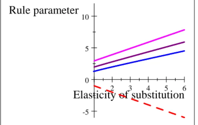
Proposition 2. For limited credibility, the in‡ation policy rule parameter F is positive. For zero-credibility, the in‡ation policy rule is negative and below -1.

Proof. One has:

1 < F ;ZC = " < 1 < 0 < F (13)

For limited credibility:

1 < F ;ZC = " < 1 < 0 < F (14)

For limited credibility, the policy rule parameter of the response to in‡ation is a de-creasing function of credibility q and an inde-creasing function of the elasticity of substitution ". To prove that the policy rule is positive, it is su¢ cient to prove:

lim q!1 "!1lim+ 1 q 0 @1 2 1 + 1 q + " q s 1 4 1 + 1 q + " q 2 1 q 1 A > 0 When q ! 1 and when " ! 1+

F 1 0 @1 2 1 + 1 + s 1 4 1 + 1 + 2 1 1 A

is true because _! max> 0 (see appendix 4A).

Figure 4. Policy rule parameters for di¤erent values of credibility q: 0 (dash line); 10 7 and 10 3 (overlap on the upper solid line); 0:5 (intermediate solid line); 1 (bot-tom solid line):

2 3 4 5 6 -5 0 5 10 Elasticity of substitution Rule parameter

3.3

Initial anchor of in‡ation on cost-push shock

Proposition 3. The initial anchor (or jump) of in‡ation on the cost-push shock is a de-creasing function of the elasticity of substitution between goods for both limited credibility and zero credibility policy regimes. It is an increasing function of the limited credibility of the policy maker.

Proof. Output gap and in‡ation are exactly linearly related at the initial date x0 =

" 0 for limited and zero-credibility case. The anchor of in‡ation on the cost-push shock

are generally di¤erent between limited credibility versus zero credibility:

0 =

1 q u0 versus 0;ZC =

1

1 + "u0

For zero credibility, the anchor of in‡ation is a decreasing function of " which is an increasing function of ". As max < " < max_L , the zero credibility initial anchor of

in‡ation ( 0=u0) is bounded: 0:81 = 1 1 + max L < 1 1 + " < lim"!1 1 1 + " = 1 1 + max = 1: 82 (15) For limited credibility, the anchor of in‡ation is a decreasing function of " which is an increasing function of ". As max < " < max

L , the zero credibility initial anchor of

in‡ation ( 0=u0) upper bound.

lim

q!1 lim"!11 q = limq!1 lim"!11 = 1:02

With: lim q!1 lim"!1 = 1 2 1 + 1 + max s 1 4 1 + 1 + max 2 1 = 0:56

The initial anchor of near-zero credibility is always strictly smaller than the initial anchor in the case of zero credibility. The gap tends to zero when the auto-correlation of the forcing variable tends to zero and when the elasticity of substitution tends to one:

! 0 and " ! 1. lim q!0+1 q = lim_q!0+ 1 1 + < 1 1 + " QED.

For Gali (2015) calibration with = 0:8 (which is far from _{! 0), for any elasticity} of substitution and for any probability of not reneging commitment, the zero credibility initial anchor of in‡ation is much higher (+80%) than the limited credibility initial anchor of in‡ation (…gure 5).

Figure 5: Initial anchor of in‡ation as a decreasing function of the elasticity of substitution for q = 0 (dash line top), q = 1 (solid line, second line from top), q = 0:5 (solid line, third curve from top), q = 10 7 _{with a value equal to the in‡ation eigenvalue}

(solid line, bottom curve) .

Figure 6: _{Initial anchor of in‡ation as an increasing function of credibility q 2 ]0; 1]} for " = 1 (top line), 6 (intermediate line) and 107 _{(bottom line).}

2 4 6 8 10 0.5 1.0 1.5 2.0 Elasticity Anchor 0.0 0.1 0.2 0.3 0.4 0.5 0.6 0.7 0.8 0.9 0.5 1.0 1.5 2.0 Credibility Anchor

As seen in …gure 6, there is a potential trade-o¤ within the cases of limited credibility: more credibility (a higher q 2 ]0; 1]) implies faster convergence on subsequent period over a longer expected duration measured by the in‡ation eigenvalue, but it allows a higher initial anchor of in‡ation which slows convergence. Which e¤ect o¤set the other is found computing impulse response functions and welfare losses in the next section.

3.4

Impulse response functions and welfare

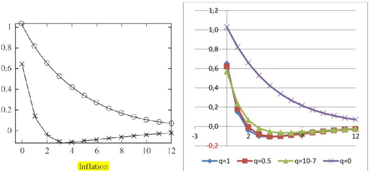
Impulse response function are shown on …gure 7 for four di¤erent degrees of credibility q: 0(for ever discretion), 10 7 _{(limit-discretion), 0:5, 1 (in…nite horizon commitment). The}

…rst impulse response of zero credibility a markedly over the impulse response functions of in‡ation with limited credibility. This is re‡ected in the evaluation of the relative welfare loss. Using table 3 formulas, we replicate Gali (2015) impulse response functions for " = 6.

Table 3: Expected impulse response functions.

Credibility Impulse response functions following u0 F Fu

q _{2 ]0; 1]} t ut = 1 q qF = 1 q qFu 0 t 1 q 1 u0 "1 1 q F q = 0 t ut = 1 _{+ "} 1 0 t ₁ 1 + " 1 u0 " 0

Welfare losses for di¤erent elasticity and di¤erent credibility computation are reported in table 4 for Gali (2015) calibration. By contrast to discretion equilibrium, we did not …nd a closed form formula for welfare losses in the case of limited credibility. Hence, we simulate the model over 200 periods in order to compute welfare. For comparison with the welfare of in…nite horizon regimes, the limited credibility welfare is arbitrarily computed using a discount factor of = 0:99 instead of q in order to take into account in a approximation the regimes which appears with probability 1 q.

Table 1: Welfare loss in percentage of welfare loss with in…nite horizon commitment (w( q) = _{W (0:99)}W ( q) 1, = 0:99, q = 1). x " = " x 2W (0:99) w(0) w(10 7) w(0:1) w(0:5) w(0:8) 10 7 _{3193 0:00032 2:119 73% 2:1% 10:8% 6:8% 2:8%} 0:02125 6 0:1275 2:688 89% 0:03% 10:9% 7:4% 3:2% 0:1 2:35 0:235 3:489 111% 8:6% 10:2% 7:8% 3:6% 0:34 1 0:34 7:971 141% 23:6% 7% 7:8% 4:1%

As seen with the impulse response functions in the case " = 6, the gap between discretion and limited commitment is very large. The loss of welfare by comparison between in…nite horizon credibility versus discretion is gigantic ranging from 60% to 118% increases of welfare losses.

When considering limited credibility taking into account the probability of not reneg-ing commitment, the losses are relatively modest (at most an increase of 24% of welfare losses in the limit case of the elasticity of substitution tending to 1) for a wide range of probabilities from 10 7 to 0:8. The welfare gap between limited credibility with a probability of not reneging commitment near zero: q = 10 7 _{versus q = 0 for discretion}

model is gigantic. For welfare evaluation, limited credibility is a very distinct model than zero credibility (discretion).

3.5

Robustness to misspeci…cation

We assume that there is a misspeci…cation by the private sector and the policy maker on their exact knowledge of parameters ; ; ; "; u0 so that the initial anchor of in‡ation 0

deviates from 10% with respect to its value with exact knowledge of parameters. This assumption is grounded by a number of major measurement issues:

1. In‡ation 0 is not measured with exact precision. This error is related to consumer

price index versus core in‡ation, quality adjusted bias and the revisions of national ac-counts.

2. A major source of new-Keynesian uncertainty is the measurement of the unob-servable cost-push shock initial value u0 depending on its past value u 1, on its

auto-correlation and on the disturbance 0. The cost-push shock is indirectly measured

an auto-correlated residual. It faces identi…cation issues when an additional lag is in-cluded for in‡ation in hybrid Phillips curve. As a residual, it varies widely depending on misspec…cation of in‡ation dynamics.

3. The estimated slope ( ; "; L; ; ; ') of the new-Keynesian Phillips curve in only

known with a standard error. It sign is even uncertain (Mavroeidis et al. (2015)). It is itself a function of six not so precisely known structural parameters ( ; "; ; ; ; '), in particular the proportion of …rms who do not reset their price at each quarter.

4. The elasticity of substitution between di¤erentiated inputs " in monopolistic com-petition which enters into welfare relative weight is not precisely known. Some authors

may refer to the measurement of Lerner index which are themselves lacking precision, with a calibration of " = 11 instead of Gali (2015) calibration of " = 6.

5. The policy maker discount factor may vary much more with a adjusted discount factor q depending on the probability q of not reoptimizing. For example, Debortoli and Lakdawala (2016) point estimate is q = 0:81_b in a 95% con…dence interval [0:777; 0:851].

Using table 3 formulas, we compute two impulse response functions of out of equilib-rium path when facing 10% error on the initial anchor of in‡ation using using Gali’s (2015) calibration.

For near zero credibility (q = 10 7), the error gap of 10% with respect to the perfect knowledge optimal path at the initial date is reduced to less than 1% after eight quarters (…gure 8).

For zero credibility (q = 0), the error gap of 10% with respect to the perfect knowl-edge optimal path at the initial date is increased to 110% after four quarters and to 270% after eight quarters (…gure 9) with in‡ation or de‡ation spirals. After six quarters, the divergence of in‡ation reaches +1% additional in‡ation with +10% error or 2% addi-tional de‡ation with 10%error with respect to the perfect knowledge impulse response function.

In the perfect knowledge case, which has a probability zero for practitioners of sta-bilization policy, the expected impulse response function may suggest that discretionary policy leans against in‡ation spirals, while using in‡ation rule parameters destabilizing the in‡ation eigenvalue. By contrast, in the imperfect knowledge case with zero cred-ibility, the outcome of discretionary policy is a probability equal to one of in‡ation or de‡ation spirals. The core behavioral hypothesis that a policy maker sticks to an ex-actly zero probability of not reneging commitment for ever is also an assumption with a probability zero for practitioners of stabilization policy.

3.6

Conclusion

Even in the most favorable case of an elasticity of substitution between goods tending to one, the limited-credibility equilibrium when the probability to renege commitment tends to zero is never the limit of the zero credibility for ever equilibrium: positive sign versus negative sign of the response of the policy instrument to in‡ation, stability versus instability of the in‡ation eigenvalue, small versus large initial anchor of in‡ation, small versus large magnitude of welfare loss, robustness versus lack of robustness to a large range of misspeci…cation and measurement error.

The bifurcation between zero credibility versus limited credibility is a general result for any linear model of the private sector with any number of lags and any number of variables including at least one forward-looking variable with a policy maker quadratic loss function. With limited credibility, the policy maker’s Lagrange multipliers of each private sector forward-looking variables are predetermined variables which are eliminated by assumption in the zero credibility model (e.g. Chatelain and Ralf (2017a)). Hence, Blanchard and Kahn (1980) determinacy condition implies more stable eigenvalues with limited credibility model with respect to zero credibility. For example, including the pri-vate sector consumption Euler equation besides the new-Keynesian Phillips curve leads to a Hopf bifurcation (Chatelain and Ralf (2017b)). This also implies that the number of non-collinear variables in a vector auto-regressive representation is smaller with zero credibility than with limited credibility (Chatelain and Ralf (2017c)). Adding more vari-ables, more lags and and more parameters in the transmission mechanism may give the

illusion that the zero credibility model may …t the data. But this result is obtained in ne-glecting exact and weak identi…cation issues and the parsimony criterion for the number of parameters when comparing models (Chatelain and Ralf (2018)).

References

[1] Blanchard O.J. and Kahn C. (1980). The solution of linear di¤erence models under rational expectations. Econometrica, 48, pp. 1305-1311.

[2] Chatelain, J. B., and Ralf, K. (2017a). A Simple Algorithm for Solving Ramsey Optimal Policy with Exogenous Forcing Variables. Paris School of Economics and SSRN working paper.

[3] Chatelain, J. B., and Ralf, K. (2017b). Hopf bifurcation from new-Keynesian Taylor rule to Ramsey optimal policy (2017). Paris School of Economics and SSRN working paper. https://papers.ssrn.com/sol3/papers.cfm?abstract_id=2971227.

[4] Chatelain, J. B., and Ralf, K. (2017c). Can we Identify Fed’s preferences? Paris School of Economics and SSRN working paper.

[5] Chatelain, J. B., and Ralf, K. (2018). Publish and Perish: Creative Destruction and Macroeconomic Theory. History of Economic Ideas, 2, forthcoming. Preprint Paris School of Economics and SSRN working paper, version 2.

[6] Debortoli, D., and Nunes, R. (2014). Monetary regime switches and central bank preferences. Journal of Money, Credit and Banking, 46(8), 1591-1626.

[7] Debortoli, D., & Lakdawala, A. (2016). How credible is the federal reserve? a struc-tural estimation of policy re-optimizations. American Economic Journal: Macroeco-nomics, 8(3), 42-76.

[8] Fujiwara, I., Kam, T., & Sunakawa, T. (2016). A note on imperfect credibility. SSRN working paper.

[9] Gali J. (2015). Monetary Policy, In‡ation, and the Business Cycle, (2nd edition) Princeton University Press.

[10] Hansen L.P. and Sargent T. (2008). Robustness, Princeton University Press, Prince-ton.

[11] Ljungqvist L. and Sargent T.J. (2012). Recursive Macroeconomic Theory. 3rd edition. The MIT Press. Cambridge, Massaschussets.

[12] Schaumburg, E., and Tambalotti, A. (2007). An investigation of the gains from commitment in monetary policy. Journal of Monetary Economics, 54(2), 302-324.

3.7

Appendix 1: Augmented Discounted Linear Quadratic

Reg-ulator

The new-Keynesian Phillips curve can be written as a function of the Lagrange multiplier where > 0, 0 < < 1 and 0 < q < 1 (Debortoli and Nunes (2014, appendix A). We keep Gali (2015) chapter 5 t+1 notation of the Lagrange multiplier with one step ahead

subscript: it corresponds to Debortoli and Nunes (2014) notation t. Our notation for

the stable eigenvalue corresponds to Debortoli and Nunes (2014) notations " y = 1= ".

Et t+1+ " q t+1 = 1 q t 1 qut 1 q q Et j t+1

In what follows, refers to q to simplify notations. The solution of the Hamiltonian system are based on the demonstrations of the augmented discounted linear quadratic regulator in Anderson, Hansen, McGrattan and Sargent [1996], following the steps in Chatelain and Ralf (2017a):

0 @ 1 " 0 0 1 0 0 0 1 1 A 0 @ t+1t+1 ut+1 1 A = 0 @ 1 ₀ 1 1 1 0 0 0 1 A 0 @ tt ut 1 A + 0 @ 1 q q Et j t+1 0 0 1 A The Hamiltonian system is:

0 @ t+1t+1 ut+1 1 A = 0 @ 1 ₊ " " 1 1 1 0 0 0 1 A 0 @ tt ut 1 A + 0 @ 1 q q Et j t+1 0 0 1 A The characteristic polynomial of this upper square matrix is:

2 _{1 +} 1 ₊ " ₊ 1 _{= 0}

The Hamiltonian matrix has two stable roots and ( is denoted in Gali (2015)) and one unstable root 1 . The determinant of the matrix is 1 = 1. Then <q1 <

1 _{. The trace of the matrix is}

= 1 2 0 @1 + 1 + " s 1 + 1 + " 2 4 1 A Policy rule parameter function of (") and ":

(1 ) 1 1 = " =₎ 1 1 = " =₎

F = 1 =

1 "

0 @ t+1t+1 ut+1 1 A = 0 @ + 1 1 1 + 1 1 1 1 1 0 0 0 1 A 0 @ t+1t+1 ut+1 1 A

Proposition A1: Solution of Ricatti and Sylvester equation: Rule parameters Pu and Pz of the response of the Lagrange multiplier on in‡ation to exogenous variables:

t= P t+ Puut (16) P = 1 1 > 0, Pu = 1 1 1 1 = 1 1 1 < 0 (17)

Demonstration: We use the method of undetermined coe¢ cients of Anderson, Hansen, McGrattan and Sargent’s (1996), section 5. The solution is the one that stabilizes the state-costate vector for any initialization of in‡ation 0 and of the exogenous variables

u0 in a stable subspace of dimension two within a space of dimension three ( t; t; ut) of

the Hamiltonian system. We seek a characterization of the Lagrange multiplier t of the

form:

t = P t+ Puut:

To deduce the control law associated with vector (P ; Pu), we substitute it into the

Hamiltonian system: 0 @ P t+1+ Pt+1 uut+1 ut+1 1 A = 0 B @ 1 _{(1 ) 1} 1 _{(1 ) 1} 1 1 1 1 0 0 0 1 C A 0 @ P t+ Pt uut ut 1 A

We write the last two equations in this system separately:

P t+1+ Puut+1= (P 1) t+ Puut ut+1= ut It follows that: t+1 = P 1 P t+ (1 ) Pu P ut

The …rst equation is such that:

t+1= 1 (1 ) 1 1 t+ (1 ) 1 1 (P t+ Puut) 1 ut Factorizing:

t+1 = 1 (1 ) 1 1 + (1 ) 1 1 P t+ (1 ) 1 1 Pu 1 ut

The method of undetermined coe¢ cients implies for the …rst term:

P 1 P = 1 + (1 ) 1 1 (P 1) P = 1 1 For the second term:

(1 ) Pu P = (1 ) 1 1 Pu 1 ) 1 = 1 1 1 + (1 ) Pu ) Pu = 1 1 1 1 ) Pu P = 1 1 = ₁ QED

Proposition A2: Optimal policy rule parameters formulas:

F = " (P 1) = "P = " 1 = 1 (18) Fu = "Pu = "P 1 = " 1 1 1 (19) Fu F = A = 1 Pu P = 1 1 = Pu P 1 = 1 + Pu P (20) Demonstration:

The …rst order condition relates Lagrange multiplier to the policy instrument:

xt = " t+1= "( t t)

xt = F t+ Fuut= "( t t) = "(P t+ Puut t))

F = "(P 1), Fu = "Pu

Proposition A3: From LQR to Gali (2015) vector basis (replace policy target by policy instrument).

One has: 1 Fu = 1 A 1 = 1 1 1 1 1 = (1 ) 1 = (1 ) A

One has: 8 > > > > < > > > > : ut+1 t+1 = 0 (1 ) A ut t + "t 0 ut xt = 1 0 AF F ut t = N ut t xt = F t+ AF ut , 8 > > > > < > > > > : ut+1 xt+1 = N 1_{(A + BF) N} ut xt + N 1 "t 0 ut t = N 1 ut xt t= _F1 xt A t One has: N 1(A + BF) N = 0 (1 ) F A

Which is Gali (2015) representation of the solution: xt = xt 1+ (1 ) F A ut 1 = xt 1+ "

1 ut 1 Proposition A4: Inequality demonstration.

One has the following inequalities

If 1 1 2( + 1 + ) + s 1 4 2 _{1 +} 1 ₊ 2 > 0 _, r 1 4(1 + + ) 2 > 1 2( 1 + + ) 1 4(1 + + ) 2 > 1 4( 1 + + ) 2 (1 + + )2 ( 1 + + )2 = 4 ( + ) > 4 + > which is true.

Figure 7: Impulse response function of inflation with q=1, 0.5, 10-7 and q=0 top curve.

Figure 8 Impulse response of inflation: q=10-7 and out of equilibrium path +/- 10% error.

Figure 9. Impulse response of inflation: q=0 and out of equilibrium path +/- 10% error. -0,2 0,0 0,2 0,4 0,6 0,8 1,0 1,2 -3 2 7 12 q=1 q=0.5 q=10-7 q=0 -0,2 -0,1 0,0 0,1 0,2 0,3 0,4 0,5 0,6 0,7 1 3 5 7 Inflation q=10-7 Error -10% Error +10% -8,0 -6,0 -4,0 -2,0 0,0 2,0 4,0 6,0 8,0 1 3 5 7 Inflation q=0 Error +10% Error -10%