HAL Id: hal-00318840
https://hal.archives-ouvertes.fr/hal-00318840
Submitted on 7 Sep 2004
HAL is a multi-disciplinary open access
archive for the deposit and dissemination of
sci-entific research documents, whether they are
pub-lished or not. The documents may come from
teaching and research institutions in France or
abroad, or from public or private research centers.
L’archive ouverte pluridisciplinaire HAL, est
destinée au dépôt et à la diffusion de documents
scientifiques de niveau recherche, publiés ou non,
émanant des établissements d’enseignement et de
recherche français ou étrangers, des laboratoires
publics ou privés.
transport model STRATAQ
B. Grassi, G. Redaelli, G. Visconti
To cite this version:
B. Grassi, G. Redaelli, G. Visconti. Assimilation of stratospheric ozone in the chemical transport
model STRATAQ. Annales Geophysicae, European Geosciences Union, 2004, 22 (8), pp.2669-2678.
�hal-00318840�
Annales Geophysicae (2004) 22: 2669–2678 SRef-ID: 1432-0576/ag/2004-22-2669 © European Geosciences Union 2004
Annales
Geophysicae
Assimilation of stratospheric ozone in the chemical transport model
STRATAQ
B. Grassi1,*, G. Redaelli1, and G. Visconti1
1Universit`a degli Studi di L’Aquila, Dipartimento di Fisica, Via Vetoio, 67010 Loc. Coppito L’Aquila, Italy *also at Universit`a degli Studi di Siena, Dipartimento di Scienze della Terra, Via del Laterino, 53100 Siena, Italy
Received: 24 October 2003 – Revised: 5 March 2004 – Accepted: 14 April 2004 – Published: 7 September 2004
Abstract. We describe a sequential assimilation approach
useful for assimilating tracer measurements into a three-dimensional chemical transport model (CTM) of the strato-sphere. The numerical code, developed largely according to Khattatov et al. (2000), uses parameterizations and sim-plifications allowing assimilation of sparse observations and the simultaneous evaluation of analysis errors, with reason-able computational requirements. Assimilation parameters are set by using χ2and OmF (Observation minus Forecast) statistics. The CTM used here is a high resolution three-dimensional model. It includes a detailed chemical pack-age and is driven by UKMO (United Kingdom Meteorolog-ical Office) analyses. We illustrate the method using assim-ilation of Upper Atmosphere Research Satellite/Microwave Limb Sounder (UARS/MLS) ozone observations for three weeks during the 1996 antarctic spring. The comparison of results from the simulations with TOMS (Total Ozone Mapping Spectrometer) measurements shows improved total ozone fields due to assimilation of MLS observations. More-over, the assimilation gives indications on a possible model weakness in reproducing polar ozone values during spring-time.
Key words. Atmospheric composition and structure
(mid-dle atmosphere-composition and chemistry; instruments and techniques)
1 Introduction
The analysis of the change in the ozone distribution, and of atmospheric chemistry in general, is severely hampered by a lack of consistent data sets. This prevents one from gain-ing insights into the role of chemistry and dynamics in de-termining the ozone distribution. These issues are usually studied by comparing observations with results from numer-ical modelling. One of the most important sources of data
Correspondence to: B. Grassi
(barbara.grassi@aquila.infn.it)
on the atmosphere are satellite measurements. Space-borne observations have the advantage of giving valuable data over much of the world; however, data resolution is usually unsat-isfactory to resolve small-scale patterns and moreover, maps of data are asynoptic because instruments collect observa-tions only along satellite tracks, and long periods of time are required to obtain a nearly complete global coverage of the Earth. On the other hand, models reproduce the chemical evolution of the atmosphere with an uncertainty due to the discretization of spatial and temporal scales, the parameter-ization of complex phenomena and the incomplete knowl-edge of some atmospheric processes. A data assimilation scheme allows us to simultaneously make use of available observations, theoretical understanding, and a priori infor-mation, within a mathematical framework. The technique seeks to produce an analysis which fits a set of observations taken over a “time window”, subject to the constraint that the evolution of the analyzed quantities is governed by a de-terministic model describing the given observations. This methodology represents a powerful tool for the understand-ing of chemical and dynamical atmospheric processes.
Data assimilation techniques are largely used for numer-ical weather prediction applications and recently have been applied to different fields of geophysical studies. Several re-search groups have demonstrated that these techniques can be very successfully applied for analysis of atmospheric chemical observations from a satellite (e.g. Fisher and Lary, 1995; Lyster et al., 1997; Khattatov et al., 2000; Stajner et al., 2001; Struthers et al., 2002) or in-situ ozone data from air-craft measurements (Cathala et al., 2003). Asynoptic satellite observations can be used to produce a set of self-consistent synoptic “chemical analyses’” of the observed species, and then, synoptic analyses can be inferred for species included within the model even though not actually observed; the methodology can also be useful for satellite instrument or model result validation.
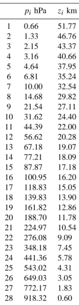
Table 1. Model levels. pi hPa zikm 1 0.66 51.77 2 1.33 46.76 3 2.15 43.37 4 3.16 40.66 5 4.64 37.95 6 6.81 35.24 7 10.00 32.54 8 14.68 29.82 9 21.54 27.11 10 31.62 24.40 11 44.39 22.00 12 56.62 20.28 13 67.18 19.07 14 77.21 18.09 15 87.87 17.18 16 100.95 16.20 17 118.83 15.05 18 139.83 13.90 19 161.82 12.86 20 188.70 11.78 21 224.97 10.54 22 276.08 9.09 23 348.18 7.45 24 441.36 5.78 25 543.02 4.31 26 649.03 3.05 27 772.17 1.83 28 918.32 0.60
The purposes of this work can be summarized as follows: a) To analyze the performance of the assimilation, by
com-paring assimilated fields and CTM model forecast with independent data set;
b) To estimate possible biases and weaknesses in the CTM model by evaluating OmF (Observation minus Forecast) differences during the assimilation cycles.
The present paper is organized as follows: the second sec-tion presents a descripsec-tion of the simulasec-tion performed; the third section describes the model and the formulation of the assimilation algorithm. The results are then presented in the following section while in the final section results are dis-cussed and summarized.
2 The simulation
As noted in the Introduction, the aim of data assimilation is to ascertain the best possible estimate of the state of a system, by combining information from observations with an appro-priate model of the system itself. A sequential assimilation algorithm, developed largely according to Khattatov et al. (2000), to assimilate measurements of long-lived species
in the stratosphere, was coupled with a three-dimensional chemical transport code of the stratosphere, which simulates the evolution of atmospheric chemical species. The result-ing system, described below, was used to assimilate UARS MLS ozone observations for a three-week period during the 1996 antarctic spring. Instruments on board UARS provided a rich set of observations of trace species concentrations in the middle atmosphere (Reber et al., 1993). We used UARS MLS level 3AT data and selected MLS ozone observations from 10 to 29 October 1996. Following Froidevaux et al. (1995), only data at UARS levels 46.4, 21.5, 10.0, 4.6, 2.1, 1.0, and 0.464 hPa, considered to be reliable, were used for the assimilation. For those seven pressure levels the relative errors, calculated from estimated precision and accuracy, are 0.23, 0.06, 0.05, 0.05, 0.06, 0.14 and 0.25, respectively. The chosen period results are particularly interesting and favor-able for two reasons:
1. Southern polar latitudes characterized by a peculiar chemical-dynamical situation (polar vortex particularly stable, leading to an “ozone hole” persisting until early December 1996);
2. Availability of 12 days of MLS data during the assimi-lation period from approximately 35◦N to about 80◦S. We also considered TOMS ozone column data for the Southern Hemisphere and HALOE (HALogen Occul-tation Experiment) ozone profiles in the middle lati-tudes, relative to the same period. Note that TOMS and HALOE data were not used in the assimilation, but con-sidered as an independent data set to validate the analy-sis results.
3 The chemical model and the assimilation scheme
3.1 STRATAQ CTM
The STRATAQ model (Grassi et al., 2002) is a three-dimensional chemistry transport model of the stratosphere that extends from 0.6 km to about 52 km in altitude with a vertical resolution varying from about 1 km below 20 km and up to 2.5 km in the higher stratosphere (see Table 1). The horizontal resolution is 5◦longitude by 2◦latitude. The chemical package includes 43 chemical species, 89 homoge-neous gas-phase chemical reactions and 33 photolytic reac-tions. To evaluate photodissociation rates J we used a “look-up table” calculated by a radiative one-dimensional model based on the delta-Eddington approximation (Joseph et al., 1976). The rate constants, as well as solar flux values and ab-sorption cross sections for chemical compounds, were taken from DeMore et al. (1997). A treatment of heterogeneous processes, occurring on the surface of stratospheric back-ground aerosols, NAT (Nitric Acid Tetrahydrate) and ice par-ticles, is included in the model. The advection, driven by the UKMO analyses, is calculated using a semi-lagrangian trans-port code (Lin and Rood, 1996). The semi-implicit symmet-ric (SIS) method (Ramaroson et al., 1992) is used to integrate
B. Grassi et al.: Assimilation of stratospheric ozone in the chemical transport model STRATAQ 2671 the chemical continuity equation. The model chemical and
dynamical time step is 12 min. For this simulation the model was initialized using output fields from long-term integration performed with the low resolution version of the 3-D SLIM-CAT CTM (Chipperfield, 1999) relative to 10 October 1996. An initial background error of 10% was fixed for the ozone field (see, e.g. Levelt et al., 1998; Struthers et al., 2002). 3.2 Assimilation scheme
In this work a sequential assimilation technique, based on the suboptimal Kalman filter, (e.g. M´enard et al., 2000), was used to evaluate the “best” value of the state of the system, or analysis Xa, which is prior information. Prior information is also given by observations Y and independent estimates of the system Xb, (also called background or “forecast” when the background is a model prediction), and by error covari-ance matrices of the background and observations. A char-acteristic feature of the Kalman filter is the computation of the time evolution of the forecast error covariance. It can be shown (e.g. Lorenc, 1986), that the expression for the analy-sis Xais given by:
Xa(t) = Xb(t) + K(Y − HXb(t)), (1) where
K = BtHT(HBtHT+O + R)−1 (2)
and H is the observation operator, which represents the trans-formation from the forecast space to the observation space and is the composition of two operators; one operator repre-sents the interpolation from the geographical locations of the model grid points to the locations of the observations while the other one denotes the relationship between the observed and estimated quantities at the geographical locations of ob-servations.
K is called the “Kalman gain matrix”. Here Btis the
fore-cast error covariance matrix at time t, O is the error covari-ance matrix of the observations and R the error covaricovari-ance matrix associated with errors of interpolation and discretiza-tion. Note that the weight given to the observations and the region influenced by each observation is properly related to the observation errors and to the background error covariance matrix. Following Lorenc (1986), the analysis error covari-ance matrix is expressed as:
Ba,t=Bt−KHBt. (3)
In our case the best estimate of the state of the atmosphere, for instance, the atmospheric ozone concentration field, is derived from a linear weighted interpolation of the vector
Xb, representing the CTM model forecast of the ozone field on the three-dimensional grid points, and the vector of ob-servations, Y , representing ozone MLS profiles along satel-lite tracks. Operatively, the Kalman filter analysis, once we have fixed a time interval called the “assimilation window” at which the analysis is performed, consists of the following steps:
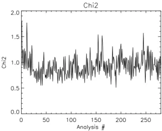
Fig. 1. Plot of <χ2>/Nas a function of time for the whole assimi-lation period. Each value is computed for one assimiassimi-lation analysis. 1. Initialize the vector X and the error covariance matrix
B;
2. Calculate the updated X and B at the beginning of the assimilation window through model integration; 3. Collect all observations Y along the assimilation
win-dow (with relative errors) and use them together with
Xb and Bt as prior information to perform the
analy-sis, following equations above in the text. Therefore, all data over the same window are assumed to be taken at the same time;
4. Then use the obtained concentrations Xa(t) as a ini-tial condition for the chemistry transport model M to predict constituent concentrations at the following time step (i.e.: the beginning of the next assimilation win-dow):
X(t+1t ) = M(Xa(t)), (4) where 1t is the time step used for the integration. Using the linearization L=∂X(t +1t )/∂t of the original model M, according to Lyster et al. (1997), in the extended Kalman filter the evolution of the error covariance matrix due to the model integration is given by:
B(t + 1t) = LBaLT. (5)
Unfortunately, such an approach is impracticable when working with an a high dimensional problem such as a three-dimensional global atmospheric system, due to the consider-able computational cost. Therefore, some parameterizations have to be introduced. Following the approach of M´enard and Chang (2000), the evolution of the diagonal element er-ror covariance matrix, bii, due to the model integration, is written as:
where xi is the i-th element of X. Therefore, B(X) is sup-posed to evolve as X itself while the second term on the right-hand side represents additional errors due to imperfections in the model.
The off-diagonal elements are parameterized as follows:
bij =pbiibjjexp(− Dxy2 2L2 xy )exp(−D 2 z 2L2 z ), (7)
where Dxyand Dzrepresent horizontal and vertical distances between locations i and j . This same parameterization is used to calculate the Ba off-diagonal elements, while only
diagonal terms are updated using Eq. (3). Moreover, matri-ces O and R are assumed to be diagonal; diagonal elements of matrix O are set to observational error variance while di-agonal elements of matrix R are parameterized as rii=(ryi)2, where r is the relative representativeness error, used as a mul-tiplying factor for the observation yi. Note that in these equa-tions Lxy, Lz, q and r are tunable parameters that can be calculated to achieve best agreement with observations us-ing the χ2 diagnostics and the OmF analysis (M´enard and Chang, 2000):
< χ2>=< (Y − H(X))T(HBHT+O + R)−1(Y − H(X)) > (8)
<OmF >=< (Y − H(X)) >
. (9)
Angular brackets denote arithmetic means calculated over different observation points in one assimilation window.
These quantities were evaluated during separate assimila-tion runs performed by setting different values of the tunable parameters. Results showed a primarily dependency of χ2 on q and r parameters; on the contrary, χ2results were quite insensitive to the value of Lxyand Lzwhich were found to influence strongly the OmF values. Based on such results, the minimization of the OmF bias was used as the base cri-teria for choosing the best value of the correlation lengths (Lxy=500. km, Lz=0.3 of the standard atmospheric scale height). The tuning procedure was performed by varying Lxy values from 300 to 3000 km and Lz values from 0.2 to 1.0 standard atmospheric scale height. Resulting OmF residu-als are presented and discussed in the next section.
Other parameters of the system, (q=0.015, r=0.13) were fixed to allow the value of <χ2>/N, where N is the num-ber of observations used in the assimilation analysis, to tend to unity and not exhibit a temporal trend (Khattatov et al., 2000). The <χ2>/N time behavior over the assimilation period is shown in Fig. 1.
The growth rate of the forecast error q and the relative representativeness error r appear to be a little bigger than in other ozone assimilations into a CTM (e.g. Khattatov et al., 2000, where q=0.0135 per hour and r=0.1). These differ-ences may be partly related to the additional interpolation of the MLS data onto STRATAQ vertical pressure levels (in Khattatov et al., 2000, vertical MLS and CTM levels coin-cided). We used an assimilation window of 1 h, correspond-ing to the time interval durcorrespond-ing which approximately 55 MLS ozone profiles were collected.
4 Results
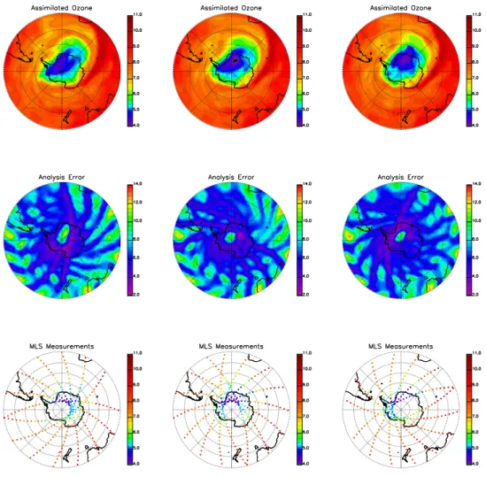
Figure 2 shows analyzed ozone fields on 29 October 1996 at 6:00, 12:00 and 18:00 UTC and relative percent analy-sis error fields. Twelve hours of MLS data, from 6 h before to 6 h after the time of analyzed fields, are also shown for comparison. All maps are relative to the 10 hPa level which represents the central level of assimilated MLS data. As ex-pected, the resulting analysis field works as an extension of MLS satellite data, originally sparse and scattered in time and space, to a regular grid for a selected time. Analyzed maps show a good comparison with MLS data. The ozone depletion inside the polar vortex recorded by the MLS in-struments is well reproduced in the analyses with minimum ozone values of about 4 ppmv. The principal maxima in ozone values at middle latitudes are also well represented. Analyzed fields seem to match well the polar vortex tilting, showing also the rapid development of a filamentary struc-ture near the antarctic peninsula. The analysis errors show values lower than 14% in the Southern Hemisphere, with maxima at low latitudes and minima in the polar region. In fact, the density of observations in this region is fairly high and this is reflected in a lower associated variance. In gen-eral, we found error values of the same order as those shown in literature (e.g. Khattatov et al., 2000).
The typical structures in the error maps show the reduction of the analysis errors along the satellite track and the increase due to the model error growth term. The tracks have a dis-torted shape reflecting the advection of the forecast standard deviation field.
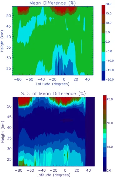
Another view of the differences between MLS observa-tions and assimilation results is shown in Fig. 3.
These plots present the monthly and zonally averaged dif-ference (top) between observations and a first guess forecast (OmF) and its standard deviation (bottom). As explained when describing the assimilation code, OmF bias was min-imized to set the correlation lengths of the forecast errors. The bias reflects data accuracy and precision and, at the same time, it is a measure of the forecast skill. The bias shows absolute values lower than 20%; it is usually below 5% be-tween approximately 30–50 km, with maximum values up to 10%, and, as expected, it grows above and below this region in correspondence to a decrease of accuracy and precision of MLS data. For the same reason, the standard deviation, whose values are lower than about 40%, shows the overall lowest values, up to 15%, between 30 to 50 km, increasing above and belove.
As seen from the type of information obtained from Fig. 3, OmF analysis provides an important quality control mecha-nism and highlights systematic differences between model results and data. Figure 4 shows another view of the same quantity. In the plot, globally averaged OmF differences (i.e. MLS minus forecast) are plotted versus time over the differ-ent pressure levels where assimilation is performed.
Within the pressure range 10.0 hPa–1.0 hPa the mean dif-ference (bias) between MLS observations and the first guess forecast is usually positive, with mean values of a few
B. Grassi et al.: Assimilation of stratospheric ozone in the chemical transport model STRATAQ 2673
Fig. 2. Results of the assimilation for October 29, 1996, at 10 hPa. Top panels: Analyzed ozone, ppmv; center panels: analysis error in percent; bottom panels: MLS measurements, ppmv. From left to right results are at 6.00, 12.00 and 18.00 UTC.
15
Fig. 2. Results of the assimilation for 29 October 1996, at 10 hPa. Top panels: Analyzed ozone, ppmv; center panels: analysis error in
percent; bottom panels: MLS measurements, ppmv. From left to right results are at 6:00, 12:00 and 18:00 UTC.
percents and maximum absolute values of less than 10%. For these levels the behavior of OmF shows a spin-up time of about 40 analysis cycles. This spin-up time, due to a bias in the initial ozone field, increases to about 60 analysis cycles at 21.6 hPa and to more than 100 analysis cycles at 0.46 hPa and 46.4 hPa. At the same time, over these three pressure lev-els, the graphics show higher OmF variability. The increas-ing spin-up time and OmF temporal variability are reason-ably related to the larger MLS observation errors at 0.46 hPa, 21.6 hPa and 46.4 hPa, which are reflected in the lower infor-mation content in the MLS observations and in model results less constrained by observations. Moreover, the spin-up time is also influenced by the ozone chemical time scale which decreases with altitude.
Analysis of Fig. 4 may give further indications about the possible origin of the higher OmF values at top and bottom assimilation levels, shown in Fig. 3, relating them to a bias in the initial (unrealistic) ozone field at the bottom level and to a standard bias in the forecast at the top level. The stan-dard bias in the forecast of about 25% at 0.46 hPa is a sign of a systematic model underestimation of ozone values on this level. Absolute values of ozone are determined mostly by
vertical transport and photochemical processes. The ozone chemical lifetime drops rapidly with altitude and, at high al-titudes, ozone levels are totally determined by the fast pho-tochemistry. Also, only a process operating on short time scales (diurnal or less) compared to the frequency of assimi-lation (about 1000 profiles a day) can maintain a systematic model bias of 25%. The diabatic descent affects ozone on very long time scales compared to the frequency of assimila-tion. On the basis of these considerations, only an incorrect estimation of the model’s fast photochemistry can explain a bias which increases with altitude.
Our assimilated field was also used to calculate the ozone total column for 29 October 1996, to be compared with ob-servations of the TOMS instrument on the NASDA/ADEOS spacecraft for the same day (Fig. 5).
To improve the comparison, the “assimilated column” is calculated at each point in the local solar time of the satel-lite measurement. TOMS data show values between 100 and 500 DU, in reasonable agreement with assimilation re-sults. The assimilated field fairly reproduces morphology and intensity of ozone depletion shown by TOMS. A quanti-tative comparison, performed on selected model grid points,
Fig. 3. Time and zonally averaged: OmF (MLS minus forecast)
mean difference (top), standard deviation from the mean (bottom). The temporal mean is calculated over all the assimilation period.
between co-located TOMS, model analysis and model only control field data is given in Fig. 6, in order to try and obtain a clearer evaluation of the performance of the assimilation.
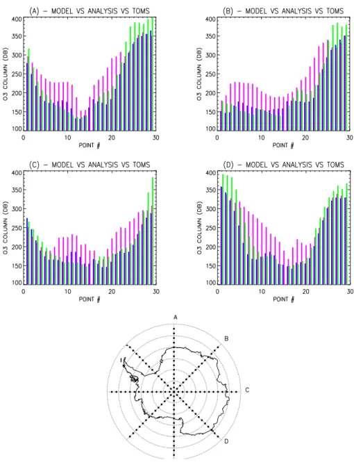
Figure 6 shows column ozone values at latitudes below
−62◦, chosen over grid points along four different directions crossing the South Pole. The comparison shows that the model field tends to overestimate column ozone values with respect to TOMS data, in the inner vortex, up to 30%. The as-similation procedure corrects the model forecast, in the right direction, toward TOMS independent data, leading to a final absolute difference between TOMS and the analyzed field of less than 10%, on average. Such results seem to confirm the hypothesis suggested in a previous work (Grassi et al., 2002) of an incorrect model estimation of the vertical velocity in the polar regions that causes an excess of ozone subsidence from higher model levels, resulting in an overestimation of ozone column values.
A slightly different behavior can be seen on the points lo-cated on the outer part of the vortex where little differences
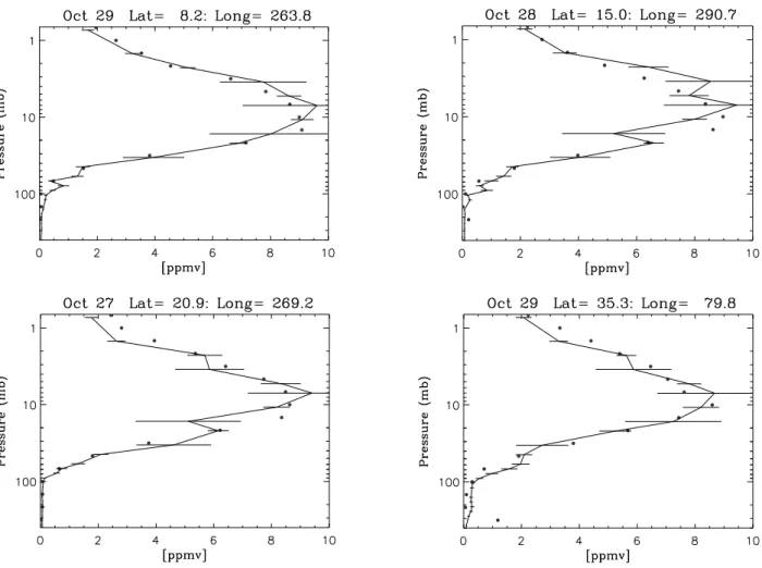
can be found between model and analyzed fields, while both showing values less than TOMS data. Those differences, of about 10%, on average, seem to be partially induced by the difficulty of correctly resolving strong meridional dynamical gradients. Also, the tropospheric contribution to the ozone column, not considered in our calculation, may be relevant at middle latitudes. An additional comparison is shown be-tween profiles from the UARS/HALOE (Halogen Occulta-tion Experiment) instrument and analysis profiles for the as-similation run (Fig. 7). The graphics refer to four differ-ent latitudes in the latitude band spanned by the instrumdiffer-ent (about 8◦–35◦N) during the last three days of the assimila-tion run.
The agreement between analysis results and independent HALOE data is fairly good if we neglect the points located above 2 mb, where the comparison seems again to highlight the existence of a model bias not removed by the assimila-tion. Different values of the error bars near the ozone maxi-mum reflect different vertical distance between the CTM lev-els and the MLS levlev-els where the assimilation is performed.
5 Conclusions
Assimilation of atmospheric chemical observations has been recently developed and used in a number of different CTMs (e.g. Errera and Fonteyn, 2001; Khattatov et al., 2000; Lamarque et al., 1999; Levelt et al., 1998; Struthers et al., 2002). In our work, a data assimilation system of chemical species coupled with STRATAQ CTM is described and pre-liminary results discussed. In this context, the computation of time evolution of the error covariance matrix is a crucial point. In our scheme this quantity was evaluated using a cer-tain number of simplifications and parameterizations. The model error growth rate was assumed to be linear. This pro-duced high values of analysis errors in the regions where a small number of assimilated observations are present, as shown in the results. The adjustable parameters, calculated to evaluate the error covariance matrix by using some mini-mization criteria, showed reliable values if compared to pre-vious similar studies.
Validation through independent observations has been per-formed on the total ozone column against TOMS data. Also, sparse ozone profiles are shown and compared with HALOE data. TOMS ozone column data give a general indication about the quality of the results; TOMS to CTM assimilated data comparison shows by itself how the assimilation tech-nique improved the CTM capability in reproducing a real at-mospheric situation. The analyses of ozone column values show an improvement of the results inside the vortex due to the assimilation leading to a reduction in the differences with TOMS data from about 25–30%, in the case of model only control values, to less than 10% in the case of assimilated values. The study of the temporal behavior of the OmF dif-ferences shows a model bias on the upper levels, suggesting an incorrect estimation of the model fast photochemistry at high altitudes.
B. Grassi et al.: Assimilation of stratospheric ozone in the chemical transport model STRATAQ 2675
Fig. 4. Globally averaged mean difference of OmF (MLS minus forecast), in percent between MLS ozone observations and co-located
analysis ozone values as a function of time for different pressure levels. Horizontal scale units are the number of assimilation cycles performed from the beginning of the run. Note the different vertical scale in the plot relative to 0.46 hPa.
Fig. 6. Ozone column values at model grid points along directions A, B, C and D, respectively (see map; for each direction 29 model grid
points from −62◦lat to −62◦lat through the South Pole are taken into account). Red and blue columns are relative to model and analysis results, respectively, while green columns are co-located TOMS values (unrealistic TOMS data on the South Pole was omitted).
Acknowledgements. We would like to thank the Upper Atmosphere
Research Satellite (UARS) Project, (Code 916), and the Distributed Active Archive Center (Code 902.2) at the Goddard Space Flight Center, Greenbelt, MD 20771 for the production and distribution of MLS and HALOE data. We thank the NASA/GSFC TOMS team for provision of TOMS data and the British Atmospheric Data Cen-tre for provision of UKMO analyses. We are grateful to M. P. Chip-perfield for kindly providing SLIMCAT CTM data used for the ini-tialization and to B. V. Khattatov for his useful suggestions in the development of the assimilation code. We also thanks two anony-mous reviewers for their useful suggestions and comments. This work has been supported by Italian Space Agency (ASI) and CNR “Agenzia 2000” program.
Topical Editor O. Boucher thanks two referees for their help in evaluating this paper.
References
Cathala, M.-L., Pailleux, J., and Peuch, V.-H.: Improving global chemical simulations of the upper troposphere – lower strato-sphere with sequential assimilation of MOZAIC data, Tellus, 55B, 1–10, 2003.
Chipperfield, M. P.: Multiannual simulations with a three-dimensional chemical transport model, J. Geophys. Res., 104, 1781–1805, 1999.
DeMore, W. B., Sander, S. P., Golden, D. M., Hampson, R. F., Howard, C. J., Ravishankara, A. R., Kolb, C. E., and Molina, M. J.: Chemical Kinetics and Photochemical Data for Use in Stratospheric Modeling, JPL publication, 97-4 JPL, Pasadena, CA, USA, 1997.
B. Grassi et al.: Assimilation of stratospheric ozone in the chemical transport model STRATAQ 2677
Fig. 7. Four examples of co-located ozone profiles (ppmv) from HALOE (solid circles) and from the assimilation system (solid line); error
bars represent corresponding analysis errors. All graphics are relative to 12:00 UTC. Errera, Q. and Fonteyn, D.: Four-dimensional variational
chemi-cal assimilation of CRISTA stratospheric measurements, J. Geo-phys. Res., 106, 12 253–12 265, 2001.
Fisher, M. and Lary, D. J.: Lagrangian 4-dimensional variational data assimilation of chemical-species, Q. J. R. Meteorol. Soc., 121(527 Part A), 1681–1704, 1995.
Froidevaux, L., Read, W. G., Lungu, T. A., Cofield, E., Fishbein, E. F., Flower, D. A., Jarnot, R. F., Ridenoure, B. P., Shippony, Z., Waters, J. W., Margitan, J. J., McDermid, I. S., Stachnik, R. A., Peckham, G. E., Braaten, G., Deshler, T., Fishman, J., Hofmann, D. J., and Oltmans, S. J.: Validation of UARS Microwave Limb Sounder ozone measurements, J. Geophys. Res., 101, 10 017– 10 060, 1995.
Grassi, B., Redaelli, G., and Visconti, G.: STRATAQ: a three-dimensional Chemical Transport Model of the stratosphere, Ann. Geophys., 20, 847–862, 2002.
Joseph, J. H., Wiscombe, W. J., and Weinman, J. A.: The delta Eddington approximation for radiative flux transfer, J. Atmos. Sci., 33, 2452–2459, 1976.
Khattatov, B. V., Lamarque, J.-F., Lyjak, L. V., M´enard, R., Levelt, P., Tie, X., Brasseur, G. P., and Gille, J. C.: Assimilation of satel-lite observations of long-lived chemical species in global chem-istry transport models, J. Geophys. Res., 105, 29 135–29 144, 2000.
Lamarque, M., Khattatov, B. V., and Gille, J. C.: Assimilation of Measurements of Air Pollution From Space (MAPS) CO in a
global three-dimensional model, J. Geophys. Res., 104, 26 209– 26 282, 1999.
Levelt, P. F., Khattatov, B. V., Gille J. C., Brasseur G. P., Tie X. X., and Waters J.: Assimilation of MLS ozone measurements in the global three-dimensional chemistry-transport model ROSE, Geophys. Res. Lett., 25, 4493–4496, 1998.
Lin, S. J. and Rood, R. B.: Multidimensional Flux-Form Semi-Lagrangian Transport Schemes, Mon. Wea. Rev., 124, 2046– 2070, 1996.
Lorenc, A. C.: Analysis methods for numerical weather prediction, Q.J.R. Meteorol. Soc., 112, 1177–1194, 1986.
Lyster, P. M., Cohn, S. E., M´enard, R., Chang, L.-P., Lin, S.-J., and Olsen, R.: An implementation of a two-dimensional filter for atmospheric chemical constituent assimilation on massively parallel computers, Mon. Weather Rev., 125, 1674–1686, 1997. M´enard, R. and Chang, L.-P.: Stratospheric assimilation of
chemi-cal tracer observations using a Kalman filter, part II: Chi-square validated results and analysis of variance and correlation dynam-ics, Mon. Weather Rev., 128, 2672–2686, 2000.
M´enard, R., Cohn, S. E., Chang, L. P., and Lyster, P. M.: Strato-spheric assimilation of chemical tracer observations using a Kalman filter, part I: Formulation, Mon. Weather Rev., 128, 2654–2671, 2000.
Ramaroson, R., Pirre, M., and Cariolle, D.: A box model for on-line computations of diurnal variations in a 1-D model: potential for application in multidimensional cases, Ann. Geophys., 10, 416–
428, 1992.
Reber, C. A., Trevathan, C. E., McNeal, R. J., and Luther, M. R.: The Upper Atmosphere Research Satellite (UARS) mission, J. Geophys. Res., 98, 10 643–10 647, 1993.
Stajner, I., Riishojgaard, L. P., and Rood, R. B.: The GEOS ozone data assimilation system: Specification of error statistics, Quart. J. Roy. Meteor. Soc., 127, 1069–1094, 2001.
Struthers, H., Brugge, R., Lahoz, W. A., O’Neill A., and Swinbank, R.: Assimilation of ozone profiles and total column measure-ments into a global General Circulation Model, J. Geophys. Res., 107, doi:10.1029/2001JD000957, 2002.