Etude de la réactivité et l’efficacité de rétention des éléments traces métalliques dans les stations d'épuration de Bordeaux et leurs apports métalliques dans les eaux de la section Garonnaise de l'estuaire de la Gironde

Texte intégral

(1)THÈSE PRÉSENTÉE POUR OBTENIR LE GRADE DE. DOCTEUR DE L’UNIVERSITÉ DE BORDEAUX ÉCOLE DOCTORALE DES SCIENCES. SPÉCIALITÉ : GÉOCHIMIE ET ÉCOTOXICOLOGIE. Par Mme Victoria Nicole DEYCARD. Etude de la réactivité et l’efficacité de rétention des éléments traces métalliques dans les stations d'épuration de Bordeaux et leurs apports métalliques dans les eaux de la section Garonnaise de l'estuaire de la Gironde. Sous la direction de : M. Gérard BLANC, (co-directeur : M. Jörg SCHÄFER) Soutenue le 23 janvier 2015 Membres du jury : M. FRANCESCHI, Michel Mme. GROSBOIS, Cécile Mme. PROBST, Anne M. LITRICO, Xavier M. VENTURA, Alexandre M. ETCHEBER, Henri. HDR- Maître de conférences Professeur HDR-Chercheur Docteur Ingénieur Chercheur. Rapporteur Rapporteur Examinateur Examinateur Invité Invité.

(2)

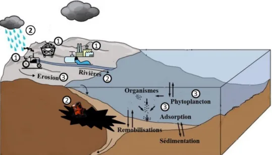
(3) Etude de la réactivité et l’efficacité de rétention des éléments traces métalliques dans les stations d'épuration de Bordeaux et leurs apports métalliques dans les eaux de la section Garonnaise de l'estuaire de la Gironde. Résumé : Cette thèse s’intègre dans l’axe 3 du programme. « ETIAGE » qui a associé pendant quatre ans (2010-2014) la Lyonnaise des Eaux, la Communauté Urbaine de Bordeaux (CUB), l’AEAG, et le FEDER, région Aquitaine avec l’université de Bordeaux, le CNRS et IRSTEA. L’objectif de l’axe 3 était de documenter les apports métalliques du bassin versant de la CUB aux eaux de la section garonnaise de l’estuaire de la Gironde. Ce vaste estuaire européen est l’un des plus turbides au monde, avec en période d’étiage la présence devant Bordeaux d’une zone de turbidité maximum (ZTM, >1 g.L-1 de MES en surface) qui transporte des particules estuariennes et des éléments traces potentiellement toxiques. Les travaux de cette thèse se sont focalisés sur les apports métalliques via le fonctionnement des deux principales stations d’épuration (STEP) de la CUB. De ce fait, l’objectif de cette recherche est d’analyser en détail les concentrations, les flux et la réactivité de huit contaminants métalliques définis comme prioritaires par l’Union Européenne Cr, Cu, Cr, Hg, Ni, Pb, Zn, As, et le contaminant émergent Ag, des STEP de la CUB. Les taux d’abattement calculés sont importants, de l’ordre de 80 % pour la majorité des métaux, essentiellement lors de l’étape de décantation. Malgré cette efficacité, les apports en éléments traces métalliques (ETM) urbains via les STEP pendant les épisodes orageux et dans des situations de faible débit peuvent augmenter les concentrations et les flux dans l’estuaire fluvial de la Gironde et ainsi avoir des conséquences sur la qualité des eaux estuariennes. Les concentrations en Ag sont supérieures aux concentrations normales de bruit de fond dans l’estuaire fluvial de la Gironde, faisant de Ag un excellent traceur urbain. Le traitement dans les STEP concentre les ETM dans les boues extraites dont les concentrations métalliques restent en-deçà des normes d’épandage. Toutefois, les concentrations en éléments traces peuvent être de 15 (Ag) à 30 (Cu) fois supérieures aux concentrations naturelles du bruit de fond en raison du fort enrichissement des boues en Hg, Ag, Cr, Cu et Zn. De plus, environ 70 % des éléments traces Cd, Ag, Pb, Cu, et Zn contenus dans ces boues sont potentiellement biodisponibles et peuvent avoir un impact néfaste à court et long terme sur les environnements récepteurs. En raison de l’augmentation prévisible de la démographie des villes côtières, les résultats de cette étude participent à l’élaboration de nouveaux concepts et outils (récupération, recyclage, valorisation) pour améliorer quantitativement et qualitativement les rejets urbains solides et liquides. Mots clés : pollution côtière, stations d’épuration, contamination estuarienne en métal trace, éléments traces métalliques urbains, flux métalliques, eaux usées, estuaire de la Gironde.

(4)

(5) The reactivity and retention of trace elements in sewage treatment plants of Bordeaux and trace metal inputs into the waters of the Garonne section of the Gironde estuary during low river discharge. Abstract : This study is a part of the third axis of the « ETIAGE » project, a four year. collaboration (2010-2014) between the Lyonnaise des Eaux, the Communauté Urbaine de Bordeaux (CUB), AEAG, and FEDER, Aquitaine region with the University of Bordeaux, CNRS and IRSTEA. The axis 3 objectives were to document the trace metal inputs from the CUB watershed into the waters of the Garonne section of the Gironde estuary. The Gironde Estuary is one of the largest macrotidal and highly turbid estuaries in Western Europe characterized by the presence of a strong maximum turbidity zone (MTZ) with high suspended particulate matter (SPM) concentrations (>1 g.L-1 in surface water) transporting estuarine particles and potentially hazardous trace elements. This study has focused on the trace metal inputs from the two main wastewater treatment plants (WWTP) of the CUB. The objective of this research was therefore to study in detail the daily concentrations, fluxes, and dynamics of 8 EU priority contaminants Cr, Cu, Cr, Hg, Ni, Pb Zn, As, and the emerging contaminant Ag from the WWTPs in the CUB. The calculated removal rates are significant, around 80 % for the majority of metals, mainly as a result of the decantation phase. Despite this high removal efficiency, during periods of heavy rainstorms and low river discharges, the urban metal inputs via the WWTPs may still significantly increase metal concentrations and fluxes in the fluvial Gironde Estuary impacting water quality. In addition, the WWTP fluxes and concentrations of Ag exceeded common background concentrations in the Gironde fluvial estuary, making it an interesting urban tracer. The treatment within the WWTPs concentrates the trace metals in the sludge, yet, metal concentrations remained below legal norms for agricultural use. However, the analysis of WWTP sludge revealed that trace element concentrations are 15 (Ag) and 30 (Cu) times higher than natural background concentrations with high enrichment of Hg, Ag, Cr, Cu and Zn with over 70 % of Cd, Ag, Pb, Cu, and Zn being potentially bioavailable. Therefore, with increasing urban pressure on environmental quality, these results support the need for the development of efficient water quality monitoring tools.. Keywords : Coastal pollution, estuary metal contamination, urban trace elements, fluxes, wastewater, Gironde Estuary. Transferts Géochimiques des Métaux à l'interface continent océan (TGM), Environnements et Paléoenvironnements Océaniques et Continentaux (EPOC)-UMR CNRS 5805 Allée Geoffroy Saint-Hilaire - CS 50023 - 33615 PESSAC CEDEX FRANCE.

(6)

(7) Acknowledgements – Remerciements Foremost, it gives me great pleasure in acknowledging the support and help of my two supervisors, Professor Gérard Blanc and Professor Jörg Schäfer. Gérard Blanc has been my guiding beacon throughout my years of doctoral research. I am truly thankful for his steadfast integrity and selﬂess dedication to my development as a researcher. I honestly cannot think of a better supervisor to have. Without a doubt, Gérard’s voice will continue to guide me long after the termination of my Ph.D with wise advice including, but not limited to, “dans la science, on ne lâche rien!”. Merci, Gérard, it was a pleasure working with you. And you were right when you said “à la fin de la thèse, tu ne seras plus la même”, and thanks to you, I now have the skills to move forward in the adventure of never having problems, only solutions. Jörg Schäfer has proven to be a great mentor from whom I have learned the vital skill of disciplined critical thinking. His forensic scrutiny of my technical writing has been invaluable. He has always found the time to propose consistently excellent improvements to which I owe a great debt of gratitude. Thanks also Jörg for reminding me every day that “bullshit" must never occur, and if it does, under no circumstances are we allowed to make excuses for it. Therefore I express my deepest thanks to both Gérard Blanc and Jörg Schäfer. Their patience, encouragement, and immense knowledge were key motivations throughout my Ph.D. I am forever grateful for my inclusion in their research team. I would also like to thank my two reporters Cécile Grosbois and Michel Fransceschi for accepting to evaluate this research, more importantly for spending their vacation doing so. I equally thank the following examiners and invited members of my defense jury: Anne Probst, Alexander Ventura, Henri Etcheber, and Xavier Litrico. It is with immense gratitude that I acknowledge the support and help of my colleague, mentor, and friend Jérôme C.J. Petit with whom I share the credit of this work. You have always provided me the priceless opportunity to exchange freely ideas regarding this Ph.D, ideas that were then transformed into scientific validation through publication. Your advice and hands-on help with the graphical presentation of data, extrapolation and synthesis of ideas from an extremely large data-set, and the publication process (writing and responding) was an essential part of this Ph.D. Thanks Jérôme for everything. I would like to also acknowledge Alexandra Coynel for oﬀering thorough and excellent feedback throughout my Ph.D and for whom I owe the unique opportunity of working with the TGM research team..

(8) I wish to thank Henri Etcheber for his thorough advice regarding all matters surrounding the production of this Ph.D and for whom I also owe the opportunity of being a part of the ETIAGE project. I also acknowledge and thank Henri for helping with the production of additional dissolved carbon data for the 2013 dataset. Thank you to all the members of the TGM team including Cécile Bossy, Lionel “Parle Français!” Dutruch, and, Laureline Gorse. You have all been a real pleasure to work with. Thank you Cécile for helping me whenever needed, especially calibrating the ICP-MS machine when it decided to act “wonky” and also for being lovely company during our Decazeville vacations, opps, sampling excursions. Thank you Lionel for your patience. Whenever “J’ai une question” you always have “peut-ȇtre une réponse”. In addition, you give the term “whistle while you work” a whole new meaning. Thanks sincerely Lionel for your guidance on all analytical procedures and equipment use in the lab and especially thanks for your help using the GC-ICPMS. A special thanks to Laureline whose help with the carbon work in this Ph.D. was invaluable. Thanks for always offering your time and assistance. You are an asset to any lab you are a part of and I am fortunate to have worked with you. A special mention to Laurent Lanceleur whose keen advice during the first half of my Ph.D. proved to be useful until the last line was written. Thank you for always sharing freely your research ideas as well as data files pertinent to the discussion of this Ph.D. In addition, thank you for your time showing me how to manage and understand my datasets, especially during the end of your own Ph.D. where time was a limited resource. I had to finish my own manuscript to truly appreciate the value of your help during that period. I cannot find words to express my gratitude to Mélina Abdou, who helped proof-read a large majority of my manuscript in French and English and whose positive moral support and friendship during the hardest times were indispensable. Thanks so much Mélina, you’re going to make an amazing academic. I consider it an honor to have worked closely next to Kahina Kessaci. It has been a growing adventure sharing an office with Kahina for 3 years and I have learned a lot through our many exchanges. Keep up the momentum my doctoral sister, it is the final stretch. In addition, I owe thanks to Aurélie Lanoux (thanks for your help in the field and sharing your figures and carbon data), Yohana Stupar (thanks for being a friend inside and outside the lab and for showing me how to use the DMA), Aurélie Larrose (thanks for your help during the end of your own Ph.D.), Lisa Bethke (thanks for your hard work acquiring the winter 2011 dataset), Emanuela Piga (your moral encouragement and friendship have been god sent this final year) and last, but never least, Jessica Villanueva (thanks for always being there to talk and reminding me to always smile, you are a true blessing to those around). Additional thanks to Stéphane Kervella for your help on my presentation during the ISOBAY conference which I used throughout the years, Eric Maneux for.

(9) your valued contribution to the ETIAGE project (updating my online publications hehe) and valuable advice, Dominique Poirier for your assistance with the dissolved carbon analysis, friendly smile and continous encouragement, Hervé Derriennic for useful field and lab assistance and Hubert Wennekes for dealing with my capricious computer “EPOC 23” who passed sadly during the final months of this work. Thank you “EPOC 23”, you will not be missed. I also thank all of the patient administrative assistants (specifically Brigitte Bordes) for their kind assistance in those matters. Thanks to all the interns and master students who worked with the TGM team. I enjoyed working next to all of you. Additional thanks to all the other doctoral students who have made this research journey feel a little less lonely. My gratitude is extended to Alexandre Ventura (SGAC/Lyonnaise des Eaux), Xavier Litrico (LyRE), as well as, Mélodie Chambolle (LyRE), Mélina Lamouroux (Agence de l’Eau Adour Garonne), Elodie Bouchon (CUB), Philippe Bourgogne, Sandrine Pelloux (SGAC/Lyonnaise des Eaux), Virginie Blasco (SGAC/Lyonnaise des Eaux), Didier Marliac (SGAC/Lyonnaise des Eaux), Emmanuel Cottin (SGAC/Lyonnaise des Eaux) and everyone at ADERA. All of your hard work towards the realization of this project is greatly appreciated and has made this research possible. Finally, I owe a debt of gratitude to my family. Thank you Muriel and Christian Deycard for all of your support, including transportation during sample collection in the summer of 2011. Thank you to my mother and father, Pietrina and Nicholas Termini. Your support emotionally and financially throughout my studies and the support of my decision to pursue a Ph.D are only a small example of the endless love you have provided for myself, my brother, and all of our spouses and children. Thanks Mom for giving me a positive role model and installing in me a strong work ethic and the importance of education. Thanks Dad for helping me live the expression, “Quitters never win and winners never quit!”. Thank you to my husband and love of my life Frédéric Deycard who worked by my side day and night on the French part of this manuscript, and after all of my mood swings, I’m still grateful to find you right there by my side. You have gone above and beyond for me and our family every day, and without your amazing mentorship, love, and companionship, this work would not have been possible, literally! And one day, I will get you that Ferrari I promised (life-sized might be difficult, but difficult never stopped either of us)..

(10)

(11) Avant-propos. Cette thèse a été réalisée dans le cadre du projet ETIAGE (Etude Intégrée de l’effet des Apports amont et locaux sur le fonctionnement de la Garonne Estuarienne) cordonné par H. ETCHEBER, P. GONTHIER, et M. LEPAGE. Elle a bénéficié du soutien financier (bourse de thèse, fonctionnement, soutien logistique) de la Lyonnaise des Eaux, de la Communauté Urbaine de Bordeaux (CUB), de l’Agence de l’Eau Adour-Garonne (AEAG) et d’une aide de la préfecture de la Région Aquitaine (FEDER). Cette thèse résulte d’une étroite collaboration entre la Lyonnaise de Eaux, l’Université de Bordeaux et le Centre National de la Recherche Scientifique (CNRS)..

(12)

(13) LISTE DES ABBREVIATIONS BTW CO COD COP CUB DCO DBO5 DOC DW EB EW EC ED EDgDs ERG ETB EH ETM F ICP-MS IW MES MO MTZ OC OM PCP POC Q SEQ SPM STEP ZTM WWTP WWTP ‘CH’ WWTP ‘LF’ (élément)D (élément)P (élément)T. Biological Treated Water Carbone Organique Carbone Organique Dissous Carbone Organique Particulaire Communauté Urbaine de Bordeaux Demande Chimique en Oxygène Demande Biologique en Oxygène Dissolved Organic Carbon Decanted Water Eau Brute Effluent Water Eau Centrifugée Eau Décantée Eau Dégraissée Dessablée Eau Rejetée dans la Garonne Eau Traitée Biologique Equivalent-Habitant Eléments Traces Métalliques flux inductively coupled plasma- mass spectrometry Influent Water Matière En Suspension Matière Organique Maximum Turbidity Zone Organic Carbon Organic Matter Personal Care Products Particulate Organic Carbon débit Système d’Evaluation de la Qualité de l’eau Suspended Particulate Matter STation d’EPuration Zone de Turbidité Maximum Wastewater Treatment Plant Wastewater Treatment Plant Clos de Hilde Wastewater Treatment Plant Louis Fargue (élément) dissous (élément) particulaire (élément) total.

(14)

(15) SOMMAIRE SOMMAIRE INTRODUCTION GÉNÉRALE ............................................................................................. 1 CHAPITRE 1 : ELEMENTS TRACES METALLIQUES (ETM). COMPORTEMENTS NATURELS ET IMPACTS ANTHROPIQUES. INTRODUCTION .............................................................................................................. 10 PARTIE I. CYCLES BIOGEOCHIMIQUES DES ETM ....................................................... 14 I.1. CYCLE ET SOURCES DES ETM DANS L’ENVIRONNEMENT .......................................... 14 I.2. QUANTIFICATION DES FLUX DE MASSE DES ETM ..................................................... 17 I.3. SPECIATION CHIMIQUE DES ETM ET FRACTIONNEMENT ........................................... 18 I.4. MOBILITE ET PROCESSUS DE TRANSFORMATION DES ETM ....................................... 21 I.5. PARTAGE ENTRE LA PHASE PARTICULAIRE ET DISSOUTE .......................................... 24 I.6. EFFET DE LA SALINITE............................................................................................... 24 I.7. ROLES DE LA TURBIDITE ET DE LA MATIERE ORGANIQUE .......................................... 25 PARTIE II. ETM ETUDIES: SOURCES ET TOXICITE ....................................................... 26 II.1. L’ARGENT (AG) ...................................................................................................... 28 II.2. L’ARSENIC (AS) ...................................................................................................... 29 II.3. LE CADMIUM (CD) .................................................................................................. 29 II.4. LE CHROME (CR) ..................................................................................................... 30 II.5. LE CUIVRE (CU) ...................................................................................................... 30 II.6. LE MERCURE (HG) .................................................................................................. 30 II.7. LE NICKEL (NI) ....................................................................................................... 31 II.8. LE PLOMB (PB) ........................................................................................................ 31 II.9. LE ZINC (ZN) ........................................................................................................... 31 PARTIE III. LES ETM DANS LES EAUX USEES URBAINES ............................................. 33 III.1. LES SOURCES DE POLLUTION .................................................................................. 33 III.2. CONCENTRATIONS EN ETM DANS LES EAUX USEES URBAINES ............................... 38 III.3. FLUX DE MASSE DES ETM DANS LES EAUX USEES URBAINES ................................. 41 CONCLUSION.................................................................................................................. 42 CHAPITRE 2 : ZONES D’ETUDES INTRODUCTION .............................................................................................................. 44 PARTIE I. LA CUB ET SON SYSTEME D’ASSAINISSEMENT ............................................ 45 I.1. LE RESEAU DE COLLECTE .......................................................................................... 45 I.2. CARACTERISTIQUES PHYSICO-CHIMIQUES DES EAUX USEES ...................................... 47 I.3. NOTION DE L’ « EQUIVALENT-HABITANT » ............................................................... 48 I.4. LES STATIONS D’EPURATION DE LA CUB. ................................................................. 50 I.5. STATION D’EPURATION LOUIS FARGUE..................................................................... 51 I.6. STATION D’EPURATION CLOS DE HILDE .................................................................... 56 I.7. TRAITEMENT DE BOUES............................................................................................. 59.

(16) SOMMAIRE PARTIE II. L’ESTUAIRE DE LA GIRONDE ...................................................................... 61 II.1. GENERALITES .......................................................................................................... 61 II.2. DYNAMIQUE DES PARTICULES ................................................................................. 64 II.3. SOURCES NATURELLES ET ANTHROPIQUES DES ETM DE L’ESTUAIRE DE LA GIRONDE ......................................................................................................................... 66 II.4. FLUX DES ETM A L’ENTREE DE L’ESTUAIRE DE LA GIRONDE .................................. 67 II.5. SPECIATION ET REACTIVITE DES ETM DANS L’ESTUAIRE FLUVIAL .......................... 69 CONCLUSION.................................................................................................................. 73 CHAPITRE 3 : CAMPAGNES DE PRELEVEMENTS, TECHNIQUES ET METHODES ANALYTIQUES DANS LES MILIEUX URBAINS ET NATURELS ETUDIES. INTRODUCTION .............................................................................................................. 76 PARTIE I. STRATEGIE D’ECHANTILLONNAGE ET CONDITIONNEMENT ........................ 76 I.1. CAMPAGNES D’ECHANTILLONNAGE DE L’EAU DES STATIONS D’EPURATION ............. 76 I.2. ECHANTILLONNAGE ET CONDITIONNEMENT DE L’EAU DES STATIONS D’EPURATION ................................................................................................................. 83 I.3. MODE DE DETERMINATION DE LA CONCENTRATION EN MATIERE EN SUSPENSION (MES) ............................................................................................................................ 88 I.4. CONCENTRATIONS EN ETM PARTICULAIRES DE L’EAU DES STATIONS D’EPURATION .................................................................................................................. 89 I.5. ECHANTILLONNAGE ET TRAITEMENT DES BOUES ET DES SABLES DES STATIONS D’EPURATION .................................................................................................................. 90 I.6. EXTRACTIONS SELECTIVES ET TOTALES DES ETM .................................................... 90 I.7. ECHANTILLONNAGE ET TRAITEMENT DE L’EAU AU SITE D’OBSERVATION DE LA REOLE ET SUR LE SITE DE BORDEAUX ............................................................................ 94 PARTIE II. METHODES ANALYTIQUES .......................................................................... 96 II.1. CARACTERISATION PHYSICO-CHIMIQUE DES EAUX .................................................. 96 II.2. ANALYSES DES CONCENTRATIONS EN ETM............................................................. 96 II.3. DOSAGE DU CARBONE ............................................................................................. 97 II.4. DOSAGE DU MERCURE PARTICULAIRE...................................................................... 98 PARTIE III. EVALUATION QUANTITATIF ET QUALITATIF DES ETM .......................... 100 III.1. CALCUL DU FLUX DES ETM ................................................................................. 100 III.2. CALCUL DE L’ABATTEMENT ................................................................................. 103 III.3. SYSTEME D’EVALUATION DE LA QUALITE DE L’EAU ............................................. 104 CONCLUSION................................................................................................................ 107.

(17) SOMMAIRE CHAPITRE 4 : ETUDE DE CONCENTRATIONS, TRANSFERTS, ET ABATTEMENT DES ETM PAR TEMPS SEC INTRODUCTION ............................................................................................................ 110 PARTIE I. CONTINUOUS 24 HOUR MONITORING OF TRACE ELEMENTS FROM INFLUENT AND BIOLOGICALLY TREATED WATER AT TREATMENT PLANT LOUIS FARGUE ........................................................................................................................ 111 I.1.1. .....CHARACTERIZATION OF TRACE ELEMENTS DURING ONE DAY MONITORING: THEIR BEHAVIOR AND POSSIBLE SOURCES ............................................................................... 111 I.2. UNDERSTANDING TREATMENT PROCESS LAG TIMES EFFECT ON TRACE ELEMENT CONCENTRATIONS: AN ARGUMENT FOR SYSTEM SPECIFIC SAMPLING STRATEGIES ........ 119 PARTIE II. THREE WEEK DRY PERIOD MONITORING OF TRACE ELEMENTS AND WATER QUALITY AT THE WASTEWATER TREATMENT PLANT LOUIS FARGUE ........... 121 II.1. DRY PERIOD DISCHARGE AND SPM ....................................................................... 121 II.2. DRY PERIOD TRACE ELEMENT CONCENTRATIONS .................................................. 122 II.3. THE USE OF METAL RATIOS TO CHARACTERIZE URBAN CONTAMINATION .............. 123 II.4. DRY PERIOD TRACE ELEMENT FLUXES ................................................................... 130 II.5. DRY TRACE ELEMENT REMOVAL ............................................................................ 134 II.6. WATER QUALITY ASSESSMENT .............................................................................. 136 CONCLUSION................................................................................................................ 138 BILAN DU CHAPITRE.................................................................................................... 139 CHAPITRE 5 : CONTRIBUTIONS ET IMPACTS POTENTIELS DE METAUX PRIORITAIRES EN PROVENANCE DES EAUX USEES DANS L’ESTUAIRE DE LA GIRONDE. INTRODUCTION ........................................................................................................... 142 PARTIE I. ARTICLE <MARINE CHEMISTRY> CONTRIBUTIONS AND POTENTIAL IMPACTS OF SEVEN PRIORITY SUBSTANCES (AS, CD, CU, CR, NI, PB, AND ZN) TO A MAJOR EUROPEAN ESTUARY (GIRONDE ESTUARY, FRANCE) FROM URBAN WASTEWATER. ............................................................................................................. 144 I.1. INTRODUCTION (<ARTICLE MARINE CHEMISTRY>) ........................................... 146 I.2. MATERIAL AND METHODS .................................................................................... 147 I.2.1. STUDY SITES ........................................................................................................ 147 I.2.2. PHYSICO-CHEMICAL WATER PARAMETERS AND SPM CONCENTRATIONS ............. 150 I.2.3. SAMPLING AND SAMPLE TREATMENT ................................................................... 151 I.2.4. ANALYTICAL METHODS ....................................................................................... 152 I.2.5. TRACE ELEMENT FLUX ESTIMATES ....................................................................... 153 I.3. RESULTS: DISSOLVED AND PARTICULATE METAL CONCENTRATIONS IN.

(18) SOMMAIRE ESTUARINE AND URBAN WASTEWATER .......................................................................... 154. I.4 DISCUSSION ............................................................................................................ 159 I.4.1. COMPARISON OF WASTEWATER INFLUENTS AND IMPACTS OF WASTEWATER EFFLUENTS ON PARTICULATE AND DISSOLVED METAL CONCENTRATIONS IN THE FLUVIAL ESTUARY ......................................................................................................... 159 I.4.2. TRACE ELEMENT PARTITIONING IN THE RIVER, THE FLUVIAL ESTUARY AND IN WASTEWATER EFFLUENTS ............................................................................................ 160 I.4.3. TRACE METAL AND AS REMOVAL DURING WASTEWATER TREATMENT ................ 166 I.4.4. TRACE METAL AND AS FLUXES INTO THE GARONNE BRANCH: WASTEWATER EFFLUENTS VERSUS RIVER TRANSPORT ......................................................................... 168. I.5. CONCLUSION AND PERSPECTIVES (<ARTICLE MARINE CHEMISTRY>).............. 174 PARTIE II. LOUIS FARGUE 2013 VS. LOUIS FARGUE 2011: AN EVALUATION OF CHANGES IN TIME AND TREATMENT ........................................................................... 176 II.1. DISCHARGE, SPM, AND PRECIPITATION ................................................................ 176 II.2. TRACE ELEMENT CONCENTRATIONS AT LOUIS FARGUE 2013 ............................... 178 II.3. COMPARISIONS OF TRACE ELEMENT CONCENTRATIONS AT LOUIS FARGUE 2013 TO LOUIS FARGUE 2011 ................................................................................................ 185 II.4. CHANGES IN ORGANIC CARBON CONCENTRATIONS AND REMOVAL ........................ 187 II.5. CHANGES IN TRACE ELEMENT REMOVAL ............................................................... 189 II.6. IMPACT ON TRACE ELEMENT FLUXES BY TREATMENT PLANT RENOVATION ........... 190 CONCLUSION <PARTIE II> ......................................................................................... 195 BILAN DU CHAPITRE.................................................................................................... 196. CHAPITRE 6 : APPORTS, DYNAMIQUES, ET IMPACTS POTENTIELS DE L’ARGENT (AG) EN PROVENANCE DES EAUX USEES URBAINES DANS L’ESTUAIRE DE LA GIRONDE (FRANCE) INTRODUCTION ............................................................................................................ 202 PARTIE I. INTRODUCTION (ARTICLE <CHEMIE DE ERDE/GEOCHEMISTRY>) ........ 206 PARTIE II. MATERIAL AND METHODS ........................................................................ 207 II.1. STUDY SITES ......................................................................................................... 207 II.2. SAMPLING AND SAMPLE TREATMENT..................................................................... 212 II.3. ANALYTICAL METHODS ........................................................................................ 213 II.4. SILVER FLUX ESTIMATES ....................................................................................... 214 PARTIE III. RESULTS ................................................................................................... 216 III.1. PERSONAL CARE PRODUCTS ................................................................................ 216 III.2. PHYSICO-CHEMICAL WATER PARAMETERS, SPM CONCENTRATIONS AND DISCHARGE IN URBAN WASTEWATER ............................................................................ 216 III.3. HOURLY AG CONCENTRATIONS IN URBAN WASTEWATER TREATMENT................. 219 III.4. DAILY AG CONCENTRATIONS IN URBAN WASTEWATER TREATMENT .................... 220.

(19) SOMMAIRE III.5. DISSOLVED AND PARTICULATE AG CONCENTRATIONS IN RIVER WATER (LA RÉOLE SITE) ................................................................................................................. 220 PARTIE IV. DISCUSSION .............................................................................................. 221 IV.1. INPUTS AND SOURCES OF AG FROM WASTEWATER .............................................. 221 IV.2. SILVER CONCENTRATIONS, REMOVAL, PARTITIONING AND FLUXES...................... 222 IV.3. SILVER DYNAMICS AND POTENTIAL IMPACTS IN RECEIVING WATERS ................... 225 PARTIE V. CONCLUSIONS AND PERSPECTIVES (ARTICLE <CHEMIE DE ERDE/GEOCHEMISTRY>)........................................................................................... 230 BILAN DU CHAPITRE .................................................................................................... 231 CHAPITRE 7 : BIODISPONIBILITE ET IMPACTS POTENTIELS DES ETM D’ORIGINE URBAINE EN PROVENANCE DES BOUES DE STATIONS D’EPURATION MUNICIPALES (CUB, FRANCE) INTRODUCTION ............................................................................................................ 234 PARTIE I. TRACE ELEMENT CONTENT AND VARIABILITY IN WASTEWATER SAND AND SEWAGE SLUDGE .................................................................................................. 236 I.1. SAND AND SLUDGE DISCHARGE FROM THE WASTEWATER TREATMENT PLANTS ...... 236 I.2. SAND AND SLUDGE TRACE ELEMENT CONCENTRATIONS ......................................... 238 PARTIE II. SAND AND SLUDGE QUALITY ASSESSMENT .............................................. 243 III.1. ENVIRONMENTAL QUALITY INDICATORS .............................................................. 243 III.2. ENRICHMENT FACTOR .......................................................................................... 254 III.3. SPECIATION AND POTENTIAL BIOAVAILABILITY ................................................... 257 PARTIE III. TRACE ELEMENT FLUXES IN WASTEWATER SAND AND SLUDGE ............ 262 CONCLUSION................................................................................................................ 265 BILAN DU CHAPITRE.................................................................................................... 266 CONCLUSIONS GENERALES ......................................................................................... 269 BIBLIOGRAPHIE ........................................................................................................... 279 VALORIZATION DE TRAVAIL ANNEXES.

(20)

(21) LISTE DES FIGURES LISTE DES FIGURES Chapitre 1 Figure 1-1: Tableau périodique des éléments avec leur toxicité (d’après Plant et al., 2001). ................................................................................................................................. 11 Figure 1-2: Sources et circulation des ETM (apports naturels internes, anthropogéniques, apports externes) dans l’environnement entre réservoirs naturels du système terrestre (modifié d’après USEPA, 2002). ...................................................... 14 Figure 1-3: Représentation graphique de l’ordre de magnitude des concentrations d’éléments traces naturels dans les charges dissoutes des fleuves (adaptation de Gaillardet et al., 2003; données argent d’après Shafer et al., 1997; Smith et Flegal, 1993; Wood et al, 2004; données mercure d’après Castelle, 2008). ................................. 15 Figure 1-4: Diagramme montrant les trois types de contamination: 1- primaire (i.e. agriculture, industrie, mine), 2- secondaire (i.e. atmosphère, ruissellement, décharge), 3- tertiaire (i.e. érosion, sédimentation, remise en suspension, réseau trophiques). .......... 17 Figure 1-5: Solubilité des éléments traces en relation avec la charge ionique et le rayon ionique (Z/r) et leurs réactions dans des environnements sédimentaires et hydrogéologiques (d’après Siegel, 2002; fondé sur Goldschmidt, 1937). ......................... 19 Figure 1-6: Distribution en taille des différentes particules et colloïdes rencontrés dans le milieu aquatique (Buffe et Van Leeuwen, 1992)................................................... 20 Figure 1-7: Diagramme pH-Eh (réduction-oxydation potentielle) montrant la relation entre les modifications de l’environnement et les changements de mobilité résultants de certains métaux potentiellement toxiques (d’après Siegel, 2002; modifié d’après Förstner, 1987 et Bourg, 1995) .............................................................................22 Figure 1-8: Droite de dilution théorique et processus d’addition et de soustraction pour un élément plus concentré en milieu marin (A) et plus concentré en milieu fluvial (B ; modifié d’après Boyle et al., 1974). ................................................................ 25 Figure 1-9: Produits courants contenant du nanoargent (source: Friends of the Earth)..................................................................................................................................26 Figure 1-10: Apports, sorties et voies de pénétration des ETM dans un système urbain (d’après Lester, 1987). ............................................................................................ 33 Figure 1-11: Concentrations de métaux d’après l’origine des ruissellements dans le quartier du Marais à Paris, un bassin versant urbain (modifié d’après Garnaud et al., 1999). ................................................................................................................................. 37 Chapitre 2 Figure 2-1: Estuaire de la Gironde avec les systèmes de la Garonne, de la Dordogne et de l’Isle. .......................................................................................................................... 44.

(22) LISTE DES FIGURES Figure 2-2: Les communes de la CUB desservies par le système d’assainissement de la CUB (Lyonnaise des Eaux, 2010; d’après Lanoux, 2013a). .......................................... 45 Figure 2-3: Schéma du système d’assainissement en 2011 (modifiée d’après Lyonnaise des Eaux, 2010). .............................................................................................. 46 Figure 2-4: Localisation des six stations d’épuration, leurs zones d’influence, capacité de traitement, et dates de mise en service et de reconstruction/réhabilitation (Lyonnaise des Eaux, 2010). .............................................................................................. 50 Figure 2-5: Courbe caractéristique du débit journalier entrant par temps sec pour l’année à Louis Fargue (Lyonnaise des Eaux, non-publié)................................................51 Figure 2-6: Schéma de la station d’épuration Louis Fargue (jusqu’en 2011) avec la position des stations de mesure du débit et les différentes étapes du traitement des eaux usées: Eau Brute (EB), Eau Dessablée et Dégraissée (EDsDg), Eau Décantée (ED), Eau Traitée Biologique (EBT,) Eau Centrifugée (EC) et Eau Rejetée vers la Garonne (ERG). ................................................................................................................. 53 Figure 2-7: Schéma de la station d’épuration Louis Fargue (après 2011) avec la position des mesures du débit et les différentes étapes du traitement des eaux usées: Eau Brute (EB), Eau Dessablée et égraissée (EDsDg), Eau Décantée (ED), Eau Traitée Biologique (ETB) Eau Centrifugée (EC) et Eau Rejetée vers la Garonne (ERG). ................................................................................................................................ 55 Figure 2-8: Courbe caractéristique du débit journalier par temps sec à Clos de Hilde (Lyonnaise des Eaux, non-publié). .................................................................................... 56 Figure 2-9: Schéma de la station d’épuration Clos de Hilde avec la position des mesures de débit et les différentes étapes du traitement des eaux usées: Eau Brute (EB), Eau Dessablée et Dégraissée (EDsDg), Eau Décantée (ED), Eau Traitée Biologique (ETB), Eau Centrifugées (EC) et Eau Rejetée vers la Garonne (ERG). ......... 58 Figure 2-10: Schéma de traitement des boues des stations d’épuration Louis Fargue et Clos de Hilde.................................................................................................................. 60 Figure 2-11: Carte de l’estuaire de la Gironde et de ses trois parties principales : estuaire fluvial, central et aval. .......................................................................................... 61 Figure 2-12: Débit moyen journalier de la Gironde, de la Garonne et de la Dordogne entre 1959 et 2012 d’après la base de données DIREN (d’après Lanoux, 2013). ............. 63 Figure 2-13: Nombre de jours où le débit de la Garonne est inférieur à 100 m3.S1 (étiage) et supérieur à 800 m3. s-1 (débit moyen, d’après Lanoux, 2013). ........................ 63 Figure 2-14: Formation du bouchon vaseux dans un estuaire macrotidial où la circulation résiduelle est faible ou absente (d’après Castaing, 1981). ............................... 64 Figure 2-15: Distribution des MES mesurées en surface et à marée basse lors de débits faibles (<300 m3.s-1) et modérés (>1000 m3.s-1 ; d’après Sottolichio et Castaing, 1999) .................................................................................................................. 65 Figure 2-16: Carte du réseau hydrographique du bassin versant de la Gironde et localisation des principaux gisements miniers (symboles des éléments) et de l’usine.

(23) LISTE DES FIGURES de traitement du minerai de Zn (étoile rouge) modifié d’après Schäfer et Blanc (2002). ................................................................................................................................ 66 Figure 2-17: Evolution du flux annuel en ETM dissous (blanc) et particulaire (gris) en t.an-1 à l’entrée de l’estuaire de la Gironde entre 1999 et 2009 (d’après Larrose, 2011). Les flux de Ag reportés correspondent aux flux mesurés sur la Garonne (Lanceleur et al., 2011a). ................................................................................................... 68 Figure 2-18: Concentrations en Cu dissous (<0,2 µm) et concentrations en MES lors des profils longitudinaux de mai (A) et septembre (B) 2005 entre La Réole et Bègles. Concentrations en Cu dissous (<0,2 µm) et en MES lors des profils longitudinaux dans le gradient de salinité de l’estuaire de la Gironde en mai (A) et juillet et novembre (B) 2005 (d’après Masson, 2007). ....................................................................70 Figure 2-19: Schéma conceptuel récapitulatif des processus affectant As, Cd, Cu, molybdène (Mo), antimoine (Sb), uranium (U) et vanadium (V) dans l’estuaire fluvial de la Gironde (source: Larrose, 2011 ; modifié d’après Masson, 2007). ...............71 Chapitre 3 Figure 3-1: Schéma des campagnes d’échantillonnage. ................................................... 77 Figure 3-2: Préleveur automatique, modèle American Sigma 900™ (A) et préleveurs réfrigérés automatiques permanents asservis aux débits installés par la Lyonnaise des Eaux (B). ...................................................................................................................... 78 Figure 3-3: Schéma d’échantillonnage pour les préleveurs automatiques permanents à Louis Fargue avant 2011. ................................................................................................ 79 Figure 3-4: Schéma d’échantillonnage pour les préleveurs automatiques permanents à Clos de Hilde. .................................................................................................................. 81 Figure 3-5: Schéma d’échantillonnage pour les préleveurs automatiques permanents à Louis Fargue après la reconstruction en 2011. ................................................................ 83 Figure 3-6: Schéma de conditionnement et d’analyses des échantillons pour la station d’épuration Louis Fargue en hiver 2010-2011. ...................................................... 85 Figure 3-7: Image de DigiPREP MS®, SCP SCIENCE avec les tubes d’attaques. .......... 86 Figure 3-8: Schéma de conditionnement et d’analyses des échantillons pour les stations d’épuration Louis Fargue et Clos de Hilde, été 2011. .......................................... 87 Figure 3-9: Schéma de protocole pour déterminer la concentration en matière en suspension (MES). ............................................................................................................. 89 Figure 3-10: Schéma du protocole des attaques sélectives parallèles et totales des boues et sable d’après de Lanceleur (2011) et Audry (2003). ........................................... 91 Figure 3-11: Schéma d’analyse et de conditionnement des échantillons des boues et sables pour les stations d’épuration Louis Fargue et Clos de Hilde 2012- 2013. ..............94 Figure 3-12: Chaîne analytique de dosage d’ETM par ICP-MS. .....................................96.

(24) LISTE DES FIGURES Figure 3-13: Chaîne analytique automatisée de dosage de Hg particulaire. .................... 99 Chapitre 4 Figure 4-1: The SPM concentrations of influent (red diamonds with dashed line) and biologically treated water (blue squares with solid line) and Influent water discharge (green triangles with dashed line) during a one day monitoring campaign. Hourly influent discharge values were calculated using yearly averages of hourly discharge by Lyonnaise de Eaux (unpublished data). ...................................................................... 111 Figure 4-2: Total (XT, µg.L-1), particulate (XP, mg.kg-1), and dissolved (XD, µg.L-1) concentrations of Cd and Pb, Particulate Organic Carbon (POC, mg.L-1 et %, Lanoux 2013) and Dissolved Organic Carbon (DOC, mg.L-1, Lanoux, 2013) during the 24 hour sampling period at WWTP Louis Fargue, where IW is denoted by red and BTW is denoted by blue symbols .............................................................................................. 113 Figure 4-3: Total (XT, µg.L-1), particulate (XP, mg.kg-1), and dissolved (XD, µg.L-1) concentrations of Cu and Zn, Particulate Organic Carbon (POC, mg.L-1 et %, Lanoux, 2013) and Dissolved Organic Carbon (DOC, mg.L-1, Lanoux, 2013) during the 24 hour sampling period at WWTP Louis Fargue, where IW is denoted by red and BTW is denoted by blue symbols.. ........................................................................... 115 Figure 4-4: Relation between POC (mg.L-1, Lanoux, 2013), DOC (mg.L-1, Lanoux, 2013), total and dissolved concentrations of Cd, Pb, Cu and Zn (µg.L-1) with SPM during the 24 hour sampling period at WWTP Louis Fargue. ......................................... 116 Figure 4-5: Demonstration of treatment time lag between IW (denoted by red color) and BTW (denoted by blue color) shown through hourly variations of dissolved Zn and Cd concentrations (µg.L-1), where estimated/extrapolated values are denoted by dashed lines and actually measured values denoted by solid lines. ................................. 119 Figure 4-6: Variations in dissolved Pb in effluent from a wastewater treatment (Marseille, France) with wastewater residence times of approximately 1h (modified from Oursel et al., 2013).. ................................................................................................ 120 Figure 4-7: (A) Discharge (IW, DW, EW, and BTW) and (B) SPM flux (influent, decanted, and biologically treated water) for the three-week winter dry period sampling. .......................................................................................................................... 121 Figure 4-8: Theoretical model signature for urban contamination. Ratios plotting close to the 1:1 line have limited potential to trace urban contamination in environmental samples.....................................................................................................125 Figure 4-9: Relation between total Cd, Pb, Cu and Zn concentrations (µg.L-1) in influent and effluent wastewater from the treatment plant Louis Fargue (Winter 2011, dry weather conditions).......................................................................................... 127 Figure 4-10: Patterns for selected metal ratios of environmental samples, WWTP samples, Upper Continental Crust composition (UCC, Rudnick and Gao, 2004), and theoretical urban signature. Metal ratios are sorted arbitraily to obtain an increasing trend for the theoritical urban signature from left to right. .............................................. 128.

(25) LISTE DES FIGURES Figure 4-11: Total, particulate, and dissolved fluxes for Cd from influent, decanted, and effluent water at the wastewater treatment plant Louis Fargue during dry weather conditions in 2011. ........................................................................................................... 130 Figure 4-12: Total, particulate, and dissolved fluxes for Pb from influent, decanted, and effluent water at the wastewater treatment plant Louis Fargue during dry weather conditions in 2011 ............................................................................................................ 131 Figure 4-13: Total, particulate, and dissolved fluxes for Cu from influent, decanted, and effluent water at the wastewater treatment plant Louis Fargue during dry weather conditions in 2011 ............................................................................................................ 132 Figure 4-14: Total, particulate, and dissolved fluxes for Zn from influent, decanted, and effluent water at the wastewater treatment plant Louis Fargue during dry weather conditions in 2011. ........................................................................................................... 133 Figure 4-15: Partitioning of average dissolved and particulate fractions of Cd, Pb, Cu and Zn in influent and effluent water total concentrations (µg.L-1) from the Louis Fargue treatment plant. ....................................................................................................135 Figure 4-16: Dry period water quality evaluation (SEQ, 2003) for Cd, Pb, Cu and Zn total (µg.L-1), dissolved (µg.L-1) and particulate (mg.kg-1) concentrations in influent, decanted and effluent wastewater from the wastewater treatment plant Louis Fargue.. . 137. Chapitre 5 Figure 5-1: Presentation of (A) the Gironde Estuary, with the Bordeaux and La Réole observation sites, (B) the Garonne Branch with the Bordeaux Urban Agglomeration (CUB) and the main wastewater treatment plants Louis Fargue (WWTP ‘LF’) and Clos de Hilde (WWTP ‘CH’). .......................................................... 148 Figure 5-2: Metal and metalloid As concentrations from the two main wastewater treatment plants (WWTP ‘LF’ denoted by red bars and WWTP ‘CH’ denoted by blue bars) during 3-week summer sampling with average value (black bars) and capped lines denoting standard deviation; (A) influent total concentration (nM), (B) effluent total concentration (nM), (C) influent particulate concentration (nmol.g-1), (D) effluent particulate concentration (nmol.g-1), (E) influent dissolved concentration (nM), (F) effluent dissolved concentration (nM). ............................................................ 157 Figure 5-3: Percent of metal and metalloid bond to particles as a function of SPM concentrations (mg.L-1) for different Log (Kd) values varying from 2 to 6 for the two treatment plants Louis Fargue (black symbols) and Clos de Hilde (white symbols) influent (IW) denoted by triangles, and effluent water (EW) denoted by squares, as well as Bordeaux (plus symbol) and La Réole (circle) sampling sites. ........................... 162 Figure 5-4: Percent metal and metalloid removal of Cd, As, Pb, Cr, Ni, Cu and Zn from the (A) total, (B) particulate, and (C) dissolved fractions of two major wastewater treatment plants Louis Fargue (WWTP ‘LF’) and Clos de Hilde (WWTP ‘CH’) discharging into the Gironde Estuary. ................................................................... 167.

(26) LISTE DES FIGURES Figure 5-5: Daily metal and metalliod flux of Cd, As, Pb, Cr, Ni, Cu and Zn (mol.d1 ) during a three week observation period in influent (A) and effluent (B) water of the two treatment plants Louis Fargue (WWTP ‘LF’) and Clos de Hilde (WWTP ‘CH’) during dry periods (0 to 1 mm precipitation) and wet periods (greater than 1 mm of precipitation). ................................................................................................................... 169 Figure 5-6: Average daily effluent metal and metalliod flux (total, dissolved, and particulate, mol d-1) for Cd, As, Pb, Cr, Ni, Cu and Zn from the two wastewater treatment plants during the three week sampling periods(maximum values denoted by capped error bar). ........................................................................................................ 170 Figure 5-7: Daily weighted averaged (mol.d-1; g.d-1) and normalized (mol.inhab-1.y1 ; g.inhab-1.y-1) metal and metalliod flux for Cd, As, Cr, Ni, Pb, Cu, and Zn released by all wastewater treatment plants of the Bordeaux Urban Agglomeration (CUB) into the Gironde Estuary compared to the minimum daily (mol.d-1; g.d-1) and normalized (mol.inhab-1.y-1; g.inhab-1.y-1) fluxes at the La Réole site. .............................................. 173 Figure 5-8: Wastewater (A) Discharge (B) SPM concentrations and (C) SPM fluxes as a function of precipitation (mm) during the three week sampling period at Louis Fargue after renovations (2013) ....................................................................................... 176 Figure 5-9: Average total, dissolved, and particulate trace element concentrations in (A) IW water, (B) DW and (C) EW water measured at Louis Fargue in 2013. .............. 179 Figure 5-10: Comparison of trace elements Cd, Ag, As, Ni, Cr, Pb, Cu and Zn in the true dissolved (<0.2µm) and colloidal fraction ( 0.2-0.02 µm) of IW (red) and EW (blue) wastewater from Louis Fargue (2013) during dry weather conditions ................. 180 Figure 5-11: Comparison of LogKd of trace elements Cr, Ag, As, Ni, Cr, Pb, Cu and Zn of IW, DW, and EW wastewater from Louis Fargue after renovations (2013). ........ 181 Figure 5-12: Comparison of average (n=12) dry period Cd, Ag, As, Ni, Cr, Pb, Cu and Zn concentrations ( Log10 +1) in the total (A), dissolved (B), and particulate (C) fraction of IW (red) and EW (blue) wastewater from Louis Fargue before (2011) and after renovations (2013) during dry weather conditions. ................................................. 185 Figure 5-13: Comparison of dissolved trace elements Cd, Ag, As, Ni, Cr, Pb, Cu and Zn in the dissolved fraction of IW (red) and EW (blue) wastewater from Louis Fargue before (2011) and after renovations (2013) during dry weather conditions, expressed in percent of total trace element concentrations.. ............................................ 187 Figure 5-14: Comparison of measured organic carbon: (A) Particulate (%) and (B) Particulate (mg.L-1) and (C) Dissolved (mg.L-1) in IW (red), DW (green), and EW (blue) wastewater from Louis Fargue before (2011) and after renovations (2013) during dry (triangle) and wet (square) weather conditions. ............................................. 189 Figure 5-15: Percent element removal at Louis Fargue before (2011) and after (2013) renovations from the (A) total (B) particulate and (C) dissolved phase .............. 189 Figure 5-16: Total (XT), dissolved (XD), and particulate (XP) IW (red) and EW (blue) trace element fluxes (g.d-1) during three week summer sampling period from the renovated Louis Fargue where capped bars represent minimum and maximum, black line denotes median, and black plus sign denotes the mean.. ................................ 191.

(27) LISTE DES FIGURES Chapitre 6 Figure 6-1: Map of studied sites including the Gironde Estuary with the Garonne, Dordogne and Isle River systems. Star represents the Bordeaux Urban Agglomeration (CUB). Black dot represents the La Réole observation site ................... 208 Figure 6-2: Scheme of the WWTP ‘Louis Fargue’. Dashed lines and arrows indicate wastewater circulation and water bypassed from decantation basins. Locations of study samplers are flanked and reported using bolded arrows. See text for definitions of acronyms ...................................................................................................................... 211 Figure 6-3: Hourly influent water ‘IW’ (A) discharge (m3.h-1) and SPM concentrations (mg.L-1). Hourly ‘IW’ and effluent water ‘EW’ Ag concentrations in the (B) total (AgT; µg.L-1), (C) particulate (AgP; mg.kg-1), and (D) dissolved (AgD; µg.L-1) fraction. ................................................................................................................ 219 Figure 6-4: Comparison of daily influent and effluent wastewater AgT, AgP and AgD fluxes (g.d-1) during wet periods (> 1 mm of precipitation) and dry periods (< 1 mm precipitation) ............................................................................................................. 223 Figure 6-5: Daily weighted averaged (g.d-1) and normalized (g.inhab-1.y-1) fluxes of AgT, AgP, AgD released by all wastewater treatment plants of the Bordeaux Urban Agglomeration (CUB) into the Gironde Estuary and the “Jalle de Blanquefort” urban watershed compared to the La Réole site. .......................................................................................................................................... 225 Figure 6-6: Percent of Ag bond to particles as a function of SPM concentrations (mg.L-1) for different Log (Kd) values varying from 2 to 6 for (A) the treatment plant Louis Fargue ‘IW’(squares) and ‘EW’(circles) and (B) sampling site near treatment plant outfall (plus signs), 2 to 80 kilometers from Bordeaux (diamonds), 80 to 130 kilometers from Bordeaux in the Gironde Estuary (triangles), and the La Reole site (minus signs) at the tidal limit ~70 kilometers upstream from Bordeaux ....................... 227 Chapitre 7 Figure 7-1: Discharge (recovery/quantities) of (A) sand (T.month-1) and (B) sludge (T.month-1) from the treatment plants Louis Fargue and Clos de Hilde .......................... 236 Figure 7-2: Destination of sewage sludge collected from all six WWTPs in the CUB from 2010 to 2013 (Lyonnaise des eaux, unpublished data)... ........................................ 237 Figure 7-3: Weight percent POC in the sludge at WWTPs Louis Fargue (red color) and Clos de Hilde (blue color) ......................................................................................... 238 Figure 7-4: Trace element concentrations for wastewater sand (A & C) and sludge (B & D) from the wastewater treatment plants Louis Fargue (denoted by red color) and Clos de Hilde (denoted by blue color) for the monthly 2012-2013 sampling period. .............................................................................................................................. 239.

(28) LISTE DES FIGURES Figure 7-5: Monthly trace element (Hg, Cd, and Ag) concentrations (mg.kg-1) in wastewater sand from Louis Fargue (denoted by red dot) and at Clos de Hilde (denoted by blue dot) compared to indicators of environmental quality (SEQ, GEODE, TEC & PEC) ..................................................................................................... 245 Figure 7-6: Monthly trace element (As, Ni, and Cr) concentrations (mg.kg-1) in wastewater sand from Louis Fargue (denoted by red dot) and at Clos de Hilde (denoted by blue dot) compared to indicators of environmental quality (SEQ, GEODE, TEC & PEC) ..................................................................................................... 247 Figure 7-7: Monthly trace element (Pb, Cu, and Zn) concentrations (mg.kg-1) in wastewater sand from Louis Fargue (denoted by red dot) and at Clos de Hilde (denoted by blue dot) compared to indicators of environmental quality (SEQ, GEODE, TEC & PEC) .....................................................................................................249 Figure 7-8: Monthly trace element (Hg, Cd and Ag) concentrations (mg.kg-1) in sewage sludge from Louis Fargue (denoted by red dot) and at Clos de Hilde (denoted by blue dot) compared indicators of environmental quality (SEQ, GEODE, TEC & PEC) ................................................................................................................................. 251 Figure 7-9: Monthly trace element (As, Ni, and Cr) concentrations (mg.kg-1) in sewage sludge from Louis Fargue (denoted by red dot) and at Clos de Hilde (denoted by blue dot) compared indicators of environmental quality (SEQ, GEODE, TEC & PEC) ................................................................................................................................. 252 Figure 7-10: Monthly trace element (As, Ni, and Cr) concentrations (mg.kg-1) in sewage sludge from Louis Fargue (denoted by red dot) and at Clos de Hilde (denoted by blue dot) compared indicators of environmental quality (SEQ, GEODE, TEC & PEC) ................................................................................................................................. 253 Figure 7-11: Percent Th in the residual fraction of wastewater sand and sludge at WWTPs Louis Fargue (red color) and Clos de Hilde (blue color) ..................................255 Figure 7-12: Average percent of trace elements associated with each selectively extracted fraction of sewage sludge from WWTPs Louis Fargue and Clos de Hilde ..... 257 Figure 7-13: Cadmium and Ag concentrations (mg.kg-1) in each selectively extracted fraction of sewage sludge from WWTPs Louis Fargue and Clos de Hilde ..................... 258 Figure 7-14: Lead, Cu, and Zn concentrations (mg.kg-1) in each selectively extracted fraction of sewage sludge from WWTPs Louis Fargue and Clos de Hilde ..................... 259 Figure 7-15: Trace element fluxes (kg.y-1) from sand at Louis Fargue (denoted by red. color) at Clos de Hilde (denoted by blue color) with montly standard deviation denoted by capped bars ........................................................................................................................ 263. Figure 7-16: Trace element fluxes (kg.y-1) from sludge at Louis Fargue (denoted by red. color) at Clos de Hilde (denoted by blue color) with monthly standard deviations denoted by capped bar.......................................................................................................................... 263. Figure 7-17: Estimated trace element fluxes (kg.y-1) of sludge and sand from all WWTPs in the CUB ......................................................................................................................... 264.

(29) LISTE DES TABLEAUX LISTE DES TABLEAUX Chapitre 1 Tableau 1-1: Emissions atmosphériques estimées dans les années 1990 (milliers de tonnes par an; d’après Larrose , 2011; modifié d’après Pacyna et Pacyna, 2001). ........... 16 Tableau 1-2: Compilation des résultats d'études portant sur la sélectivité de différents sortants pour les métaux (d’après Petit, 2003). ................................................ 23 Tableau 1-3: Les 9 ETM étudiés, sources naturelles, sources anthropiques et formes communes dans les déchets industriels urbains (d’après Andriano, 2001; Mandarino et Back, 2004; modifié d’après Sparks, 2005). ................................................................. 27 Tableau 1-4: Les 9 ETM étudiés, leur rôle métabolique, toxicités réelles ou potentielles (d’après Siegal, 2002; modifié d’après Fergusson, 1990 et Merian, 1991) ..................................................................................................................................28 Tableau 1-5: Pourcentage des ETM potentiellement toxiques dans les eaux usées de sources diverses en France (ADEME, 1995). ....................................................................34 Tableau 1-6: Sources domestiques d’ETM potentiellement toxiques dans les eaux usées européennes (d’après ECR, 2001 et Lester, 1987; modifié d’après WRc, 1994). ... 35 Tableau 1-7: Sources commerciales d’ETM potentiellement toxiques dans les eaux usées de différents pays européens (modifié d’après ECR, 2001)..................................... 36 Tableau 1-8: Concentrations moyennes des affluents et effluents (en µg.L-1) de différentes STEP dans le monde. . ..................................................................................... 40 Tableau 1-9: Données des flux en ETM (grammes par jour, g.j-1) des rejets de STEP mixtes ou industrielles en France (modifié d’après INERIS, 2008). ............................... 41 Chapitre 2 Tableau 2-1: Caractéristiques hydrologiques de la Garonne et de la Dordogne (DIREN, 2012). .................................................................................................................. 62 Tableau 2-2: Références utilisées dans la synthèse des flux en ETM entrant dans l’estuaire. ............................................................................................................................ 67 Tableau 2-3: Synthèse des comportements et processus affectant les ETM (Ag, As, Cd, Cu, et Ni) dans l’estuaire fluvial de l’estuaire de la Gironde (Garonne). ................... 72 Chapitre 3 Tableau 3-1: SEQ concentrations des micropolluants de la fraction dissoute (µg.L-1, d’après SEQ-Eau, 2003). ................................................................................................. 105 Tableau 3-2: SEQ concentrations des micropolluants de la fraction particulaire (mg.kg-1, d’après SEQ-Eau, 2003). ................................................................................. 105.

(30) LISTE DES TABLEAUX Chapitre 4 Tableau 4-1: Spearman nonparametric correlation variance matrix for total and dissolved element concentrations in hourly samples IW and BTW from Louis Fargue treatment plant in winter 2011 (dry conditions). ............................................................. 118 Tableau 4-2: Dry period Cd, Pb, Cu and Zn total (µg.L-1), dissolved (µg.L-1) and particulate (mg.kg-1) concentrations in IW, DW, and EW from the wastewater treatment plant Louis Fargue ........................................................................................... 122 Tableau 4-3: Purification performance of the Louis Fargue treatment plant during dry conditions (winter, 2011) for the overall, decantation and biological treatment on the total, particulate, and dissolved fraction of the trace elements Zn, Cu, Pb, and Cd. . 134 Chapitre 5 Tableau 5-1: Environmental parameters of the influent and effluent of the wastewater treatment facilities, and the La Réole and Bordeaux sampling sites ............ 151 Tableau 5-2: Mean, minimum, maximum concentration values at the La Réole (2011) and Bordeaux (2008) sampling sites for particulate (nmol.g-1; mg.kg-1) and dissolved (nM; µg.L-1) Cd, As, Pb, Cr, Ni, Cu and Zn (P = particulate and D = dissolved). ........................................................................................................................ 155 Tableau 5-3: Mean and standard deviation of Kd values at La Réole (2011) and Bordeaux (2008) sampling sites for Cd, As, Pb, Cr, Ni, Cu and Zn. ............................... 163 Tableau 5-4: Minimum flux values in mol.d-1 (kg.d-1) at the La Réole site in 2011 for total Cd, As, Pb, Cr, Ni, Cu and Zn (T = total, P = particulate and D = dissolved) with respective river discharge (m3.s-1) and the month measured. .................................. 171 Tableau 5-5: Average total, dissolved, and particulate trace element concentrations in IW, DW, and EW measured at Louis Fargue in 2013. ................................................ 178 Tableau 5-6: Total (µg.L-1), dissolved (µg.L-1), and particulate (mg.kg-1) Cd, Ag, As, Ni and particulate (mg.kg-1) Hg concentrations in IW, DW and EW from Louis Fargue 2013 (after renovations), Louis Fargue 2011 (before renovations) during dry (< 1mm precipitation) and wet (> 1mm precipitation) weather conditions ..................... 183 Tableau 5-7: Total (µg.L-1), dissolved (µg.L-1), and particulate (mg.kg-1) Cr, Pb, Cu, and Zn concentrations in IW, DW and EW from Louis Fargue 2013 (after renovations) and Louis Fargue 2011 (before renovations) during dry (< 1mm precipitation) and wet (> 1mm precipitation) weather conditions ................................... 184 Tableau 5-8: Trace element fluxes (total and dissolved fraction) from wastewater (IW and EW) for the entire CUB before Louis Fargue renovations ............................... 192 Tableau 5-9: Trace element fluxes (total and dissolved fraction) from wastewater (IW and EW) for the entire CUB after Louis Fargue renovations .................................. 193 Tableau 5-10: Trace element fluxes normalized by population for the CUB and the Seine Aval WWTP in Paris, France (Buzier et al., 2010; total and dissolved fraction) from influent wastewater ................................................................................................ 194.

(31) LISTE DES TABLEAUX Chapitre 6 Tableau 6-1: Water temperature (°C), pH, Electrical Conductivity (µS.cm-1), POC (mg.L-1; %) and DOC (mg.L-1) concentrations for influent, decanted, and biologically treated wastewater........................................................................................ 216 Tableau 6-2: Average total (µg.L-1), dissolved (µg.L-1), and particulate (mg.kg-1) Ag, SPM (mg.L-1) and discharges (m3.d-1) of influent, decanted, and effluent wastewater for daily sampling campaigns during a three week winter dry period and a three week summer rainstorm period ........................................................................... 218 Chapitre 7 Tableau 7-1: Local background trace element concentrations (mg.kg-1) in sediments and French limits for sludge use in agriculture (Arrêté 08/01/98) compared to trace element concentrations (mg.kg-1) in wastewater sand, sludge, sludge compost, and pipe residue ...................................................................................................................... 240 Tableau 7-2: Trace element concentrations in marine/estuarine sediments classified by the GEODE as Level 1 and 2 contamination (Arrêté du 14/06/2000). ....................... 243 Tableau 7-3: Trace element concentrations from freshwater sediment quality guidelines TEC and PEC (Mac Donald et al., 2000). ...................................................... 244 Tableau 7-4: Enrichment factors of trace elements in sewage sludge of the two WWTPs, Clos de Hilde and Louis Fargue, sewage sludge compost, and pipe residue from Louis Fargue............................................................................................................256 Tableau 7-5: Trace element fluxes from sand and sludge (sum of both WWTPs) ........ 262.

(32)

(33) INTRODUCTION GENERALE. INTRODUCTION GENERALE. 1.