The JCMT Gould Belt Survey: a first look at IC 5146

Publisher’s version / Version de l'éditeur:

The Astrophysical Journal, 836, 1, 2017-02-10

READ THESE TERMS AND CONDITIONS CAREFULLY BEFORE USING THIS WEBSITE. https://nrc-publications.canada.ca/eng/copyright

Vous avez des questions? Nous pouvons vous aider. Pour communiquer directement avec un auteur, consultez la première page de la revue dans laquelle son article a été publié afin de trouver ses coordonnées. Si vous n’arrivez pas à les repérer, communiquez avec nous à PublicationsArchive-ArchivesPublications@nrc-cnrc.gc.ca.

Questions? Contact the NRC Publications Archive team at

PublicationsArchive-ArchivesPublications@nrc-cnrc.gc.ca. If you wish to email the authors directly, please see the first page of the publication for their contact information.

NRC Publications Archive

Archives des publications du CNRC

This publication could be one of several versions: author’s original, accepted manuscript or the publisher’s version. / La version de cette publication peut être l’une des suivantes : la version prépublication de l’auteur, la version acceptée du manuscrit ou la version de l’éditeur.

For the publisher’s version, please access the DOI link below./ Pour consulter la version de l’éditeur, utilisez le lien DOI ci-dessous.

https://doi.org/10.3847/1538-4357/aa5b95

Access and use of this website and the material on it are subject to the Terms and Conditions set forth at

The JCMT Gould Belt Survey: a first look at IC 5146

Johnstone, D.; Ciccone, S.; Kirk, H.; Mairs, S.; Buckle, J.; Berry, D. S.;

Broekhoven-Fiene, H.; Currie, M. J.; Hatchell, J.; Jenness, T.; Mottram, J. C.;

Pattle, K.; Tisi, S.; Di Francesco, J.; Hogerheijde, M. R.; Ward-Thompson,

D.; Bastien, P.; Bresnahan, D.; Butner, H.; Chen, M.; Chrysostomou, A.;

Coudé, S.; Davis, C. J.; Drabek-Maunder, E.; Duarte-Cabral, A.; Fich, M.;

Fiege, J.; Friberg, P.; Friesen, R.; Fuller, G. A.; Graves, S.; Greaves, J.;

Gregson, J.; Holland, W.; Joncas, G.; Kirk, J. M.; Knee, L. B. G.; Marsh, K.;

Matthews, B. C.; Moriarty-Schieven, G.; Mowat, C.; Nutter, D.; Pineda, J. E.;

Salji, C.; Rawlings, J.; Richer, J.; Robertson, D.; Rosolowsky, E.; Rumble, D.;

https://publications-cnrc.canada.ca/fra/droits

L’accès à ce site Web et l’utilisation de son contenu sont assujettis aux conditions présentées dans le site LISEZ CES CONDITIONS ATTENTIVEMENT AVANT D’UTILISER CE SITE WEB.

NRC Publications Record / Notice d'Archives des publications de CNRC:

The JCMT Gould Belt Survey: A First Look at IC 5146

D. Johnstone1,2, S. Ciccone1,3, H. Kirk1, S. Mairs1,2, J. Buckle4,5, D. S. Berry6, H. Broekhoven-Fiene1,2, M. J. Currie6, J. Hatchell7, T. Jenness8, J. C. Mottram9,10, K. Pattle11, S. Tisi12, J. Di Francesco1,2, M. R. Hogerheijde9, D. Ward-Thompson11, P. Bastien13, D. Bresnahan11, H. Butner14, M. Chen1,2, A. Chrysostomou15, S. Coudé13, C. J. Davis16, E. Drabek-Maunder17, A. Duarte-Cabral7,

M. Fich12, J. Fiege18, P. Friberg6, R. Friesen19, G. A. Fuller20, S. Graves6, J. Greaves21, J. Gregson22,23, W. Holland24,25, G. Joncas26, J. M. Kirk11, L. B. G. Knee1, K. Marsh27, B. C. Matthews1,2, G. Moriarty-Schieven1, C. Mowat7, D. Nutter27, J. E. Pineda20,28,29, C. Salji4,5, J. Rawlings30, J. Richer4,5, D. Robertson3, E. Rosolowsky31, D. Rumble7, S. Sadavoy10, H. Thomas6,

N. Tothill32, S. Viti30, G. J. White22,23, J. Wouterloot6, J. Yates30, and M. Zhu33

1

NRC Herzberg Astronomy and Astrophysics, 5071 West Saanich Road, Victoria, BC, V9E 2E7, Canada

2

Department of Physics and Astronomy, University of Victoria, Victoria, BC, V8P 1A1, Canada

3

Department of Physics and Astronomy, McMaster University, Hamilton, ON, L8S 4M1, Canada

4

Astrophysics Group, Cavendish Laboratory, JJThomson Avenue, Cambridge, CB3 0HE, UK

5

Kavli Institute for Cosmology, Institute of Astronomy, University of Cambridge, Madingley Road, Cambridge, CB3 0HA, UK

6

East Asian Observatory, 660 North A‘ohōkū Place, University Park, Hilo, Hawaii 96720, USA

7_{Physics and Astronomy, University of Exeter, Stocker Road, Exeter EX4 4QL, UK} 8

Large Synoptic Survey Telescope Project Office, 933 N. Cherry Avenue, Tucson, Arizona 85721, USA

9

Leiden Observatory, Leiden University, P.O. Box 9513, 2300 RA Leiden, The Netherlands

10

Max Planck Institute for Astronomy, Königstuhl 17, D-69117 Heidelberg, Germany

11

Jeremiah Horrocks Institute, University of Central Lancashire, Preston, Lancashire, PR1 2HE, UK

12

Department of Physics and Astronomy, University of Waterloo, Waterloo, Ontario, N2L 3G1, Canada

13

Université de Montréal, Centre de Recherche en Astrophysique du Québec et département de physique, C.P. 6128, succ.centre-ville, Montréal, QC, H3C 3J7, Canada

14

James Madison University, Harrisonburg, Virginia 22807, USA

15

School of Physics, Astronomy & Mathematics, University of Hertfordshire, College Lane, Hatfield, Herts, AL10 9AB, UK

16

Astrophysics Research Institute, Liverpool John Moores University, Egerton Warf, Birkenhead, CH41 1LD, UK

17_{Imperial College London, Blackett Laboratory, Prince Consort Road, London SW7 2BB, UK} 18

Departmentof Physics & Astronomy, University of Manitoba, Winnipeg, Manitoba, R3T 2N2, Canada

19

Dunlap Institute for Astronomy & Astrophysics, University of Toronto, 50 St. George Street, Toronto ON M5S 3H4 Canada

20

Jodrell Bank Centre for Astrophysics, Alan Turing Building, School of Physics and Astronomy, University of Manchester, Oxford Road, Manchester, M13 9PL, UK

21

Physics & Astronomy, University of St.Andrews, North Haugh, St. Andrews, Fife KY16 9SS, UK

22

Departmentof Physical Sciences, The Open University, Milton Keynes MK7 6AA, UK

23

The Rutherford Appleton Laboratory, Chilton, Didcot, OX11 0NL, UK

24

UK Astronomy Technology Centre, Royal Observatory, Blackford Hill, Edinburgh EH9 3HJ, UK

25_{Institute for Astronomy, Royal Observatory, University of Edinburgh, Blackford Hill, Edinburgh EH9 3HJ, UK} 26

Centre de recherche en astrophysique du Québec et Département de physique, de génie physique et d’optique, Université Laval, 1045 avenue de la médecine, Québec, G1V 0A6, Canada

27

School of Physics and Astronomy, Cardiff University, The Parade, Cardiff, CF24 3AA, UK

28

European Southern Observatory (ESO), Garching, Germany

29

Max Planck Institute for Extraterrestrial Physics, Giessenbachstrasse 1, D-85748 Garching, Germany

30

Department of Physics and Astronomy, UCL, Gower Street, London, WC1E 6BT, UK

31

Department of Physics, University of Alberta, Edmonton, AB T6G 2E1, Canada

32

University of Western Sydney, Locked Bag 1797, Penrith NSW 2751, Australia

33

National Astronomical Observatory of China, 20A Datun Road, Chaoyang District, Beijing 100012, China Received 2016 October 3; revised 2016 December 16; accepted 2017 January 3; published 2017 February 14

Abstract

We present 450 and 850 μm submillimeter continuum observations of the IC 5146 star-forming region taken as part of the James Clerk Maxwell Telescope Gould Belt Survey. We investigate the location of bright submillimeter (_{clumped) emission with the larger-scale molecular cloud through comparison with extinction maps, and find that} these denser structures correlate with higher cloud column density. Ninety-six individual submillimeter clumps are identified using FellWalker,and their physical properties are examined. These clumps are found to be relatively massive, ranging from 0.5M to 116M with a mean mass of 8 M and a median mass of 3.7 M . A stability

analysis for the clumps suggests that the majority are (thermally) Jeans stable, withM MJ<1. We further compare the locations of known protostars with the observed submillimeter emission, finding that younger protostars, i.e., Class 0 and I sources, are strongly correlated with submillimeter peaks and that the clumps with protostars are among the most Jeans unstable. Finally, we contrast the evolutionary conditions in the two major star-forming regions within IC 5146: the young cluster associated with the Cocoon Nebula and the more distributed star formation associated with the Northern Streamer filaments. The Cocoon Nebula appears to have converted a higher fraction of its mass into dense clumps and protostars, the clumps are more likely to be Jeans unstable, and a larger fraction of these remaining clumps contain embedded protostars. The Northern Streamer, however, has a larger number of clumps in total and a larger fraction of the known protostars are still embedded within these clumps.

Key words:_{ISM: clouds – ISM: structure – stars: formation – stars: protostars – submillimeter: galaxies –} submillimeter: ISM

836:132 (21pp), 2017 February 10 https://doi.org/10.3847/1538-4357/aa5b95

1. Introduction

The Gould Belt Legacy Survey (GBS; Ward-Thompson et al.

2007) conducted with the James Clerk Maxwell Telescope (JCMT) extensively observed many nearby star-forming regions, tracing the very earliest stages of star formation at 450 and 850 μm with the Submillimetre Common-User Bolometer Array 2 (SCUBA-2; Holland et al. 2006). This imaging covered 50 square degrees of nearby clouds within the Gould Belt, including

well-known regions such as Auriga (Broekhoven-Fiene

et al. 2016), Ophiuchus (Pattle et al. 2015), Orion (Salji et al.

2015a,2015b; Kirk et al.2016a,2016b; Lane et al.2016; Mairs et al.2016), Perseus (Hatchell et al.2013; Sadavoy et al.2013; Chen et al. 2016), SerpensMWC297 (Rumble et al. 2015), Taurus (Buckle et al. 2015; Ward-Thompson et al.2016), and W40 (Rumble et al.2016). Among these targets, the GBS survey covered approximately 2.5 square degrees of the IC 5146 star-forming region.

The molecular cloud, IC 5146, is both a reflection nebula and

an HII region surrounding the B0 V Star BD+46° 3474

(Herbig & Reipurth2008, see their Figures 1 and 2). IC 5146 is comprised of two notable features: the first being the Cocoon Nebula, which is a bright core nebula located within a bulbous dark cloud at the end of a long filamentary second feature, the Northern Streamer, extending northwest from the Cocoon Nebula. These two features display distinctly different proper-ties, clustered versus distributed young stars, and therefore present an ideal laboratory for investigating the range of star-formation processes within a single cloud.

In this paper, we take a first look at the submillimeter continuum emission within IC 5146, concentrating on the distribution of dense gas and dust within the cloud and its relation with on-going star formation. In Section2, we provide background information on IC 5146 and its two main features. The new SCUBA-2 observations along with estimates of the total cloud column density and protostellar content are discussed in Section 3. These observations are analyzed in Section4, starting from the largest physical scales and zooming in through the submillimeter clumps to the individual young stellar objects (YSOs). Section 5 adds context to the analysis, contrasting star formation in the Cocoon Nebula and the Northern Streamer filaments, and the results are summarized in Section 6.

2. IC 5146

There are varying estimates of the distance to IC 5146. Initially, a distance of 1000 pc was determined by Walker (1959) using photoelectric star observations. A distance of 460pc was later derived by Lada et al. (1999)using deep near-infrared (HK) imaging observations to compare the number of foreground stars to those expected from galactic models. Herbig & Reipurth (2008)adopt a distance of 1200±180 pc in their review based on the work of Herbig & Dahm (2002) that used spectroscopic distances to late-B stars and two different main-sequence calibrations. An estimation of 1200pc is quite high in comparison to the Lada estimation but nearer to initial stellar distances measured by Walker (1959)and Elias (1978). For their Spitzer Space Telescope analysis of IC 5146, Harvey et al. (2008) re-evaluated the photometric distance using a modern ZAMS calibrator, the Orion Nebula Cluster, and several photometric methods for different members of

IC 5146. A distance of 950±80 pc was determined by their analysis and, for consistency with that paper, we use 950 pc throughout the rest of this work.

IC 5146 consists of many distinct populations across two main features, the Cocoon Nebula and the Northern Streamer. Optical and near-infrared identified objects include approximately 20 variable stars, 40 faint stars above the main sequence that are the members of a population of young pre-main-sequence stars, 100 Hα-emission stars (Herbig & Dahm 2002), 110M>1.2M

stars (Forte & Orsatti1984), and 200 candidate YSOs (Harvey et al. 2008). Using WISE data in combination with existing

Spitzerand Two Micron All Sky Survey (2MASS) observations,

Nunes et al. (2016)identify new candidate YSOs in the extended IC5146 region, including five protostellar clusters (with ∼20–50 members each) in the area around the Northern Streamer, as well as a total of ∼160 protostars within the cluster at the centerof the Cocoon Nebula. The more-evolved stars of the Cocoon Nebula complex are thought to be spatially co-distant with the younger stars still entangled within the current dense gas. Two discrepancies to this claim are the distances determined for BD+46° 3471 and BD+46° 3474 as 355 pc and 400 pc respectively (Harvey et al. 2008). These distances, as well as the Lada et al. (1999)distance of 460 pc, remain problematic because at approximately 400 pc the ages of the K/M-type T Tauri stars in the cluster jump from 0.2 to 15 Myr (Harvey et al. 2008). The later isochronal age is inconsistent with the fact that IC 5146 has a high number of accreting pre-main-sequence stars, as well as the appearance of nebulosity observed in the region. Indeed, this evidence of on-going star formation argues for an age of less than a few megayearsfor the region. There is also strong circumstantial evidence that the two main components of IC 5146, the Cocoon Nebula and the Northern Streamer, are co-distant. First, the Cocoon Nebula appears to be connected to a long filament with the Northern Streamer forming at the opposite end. Second, the molecular gas associated with the Cocoon Nebula has velocities consistent with those seen in the rest of the IC 5146 region (Dobashi et al.1993).

The total H2 molecular mass of the central IC 5146 cloud

complex has been estimated to be approximately 4000M,

similar to that of the Taurus complex, as measured by Dobashi et al. (1992,1993)using12CO(J= -1 0),13CO(J= -1 0), and C18O(J= -1 0)emission lines. The total mass estimates of HIand HII, respectively, are approximately670Mand4.5M

as determined by Samson (1975) or 445105M and

 M

9.8 1 as determined by Roger & Irwin (1982). All of these mass estimates were made assuming a distance to the cloud of approximately 1 kpc. The median age for the cluster, based on isochrone fits to the optical and near-infrared pre-main-sequence stars, is approximately 1.0 Myr (Herbig & Dahm2002; Herbig & Reipurth 2008), in rough agreement with the young ages determined for the K/M-type T Tauri stars.

2.1. The Cocoon Nebula

The molecular cloud structure southeast of the Northern Streamer is noticeably bright and active due in part to the presence of BD+46° 3474 and the high-luminosity variable star V1735 Cyg from which X-ray emission has been detected (Skinner et al.2009).

The Cocoon is a more-evolved HII star-forming region relative to younger complexes found in the Orion or Ophiuchus

clouds, showing decreased small-scale structure due to density inhomogeneities expanding into more diffuse surroundings (Israel1977; Wilking et al.1984). The dust has dispersed into a mottled structure, as evidenced from scattered light, suggesting that the collective activity of the stars in this region has blown out material from the center. There is further evidence of dispersal due to the presence of BD+46° 3474 itself, which is the most massive star in IC 5146 and is responsible for the observed gas and dust emission surrounding the HII region (Wilking et al.1984). Cluster stars appear to have formed in a dense foreground section of the molecular cloud. BD+46° 3474, however, has evacuated a blister cavity out of which gas and dust are now flowing through a funnel-shaped volume and dissipating the cloud region (Herbig & Dahm2002).

More than 200 YSO candidates have been identified throughout IC 5146 using observations from the Spitzer Space

Telescope, and the population near the Cocoon Nebula is more

evolved, based on spectral observations, when compared to the younger YSOs found in the Northern Streamer (Harvey et al.2008)_{. High-velocity CO outflows were identified around} many protostellar candidates, based on the IRAS Point Source Catalog (Dobashi et al. 1993,2001). Thus, this region of the molecular cloud remains active, exhibiting an extended period of development.

2.2. The Northern Streamer

The Northern Streamer is comprised of a network of near-parallel filaments in which star formation is occurring. Twenty-seven filaments were identified using Herschel continuum data and traced throughout the region (Arzoumanian et al. 2011). The observed substructure within these filaments suggests that they are the primary birth sites of prestellar cores (Di Francesco 2012; Polychroni et al. 2013). We identify both cores and YSOs along the filamentary sections of the streamer (see Sections 4.2 and 4.3), supporting the notion that here large-scale filament morphology plays a role in the production of stars.

In this paper, we do not characterize or identify any singular filamentary structures by a modeling algorithm, but we do study and analyze the general morphology of the filamentary and clump structures seen in the streamer. Recently, Pon et al. (2011,2012)_{showed that filamentary geometry at this scale is} the most favorable scenario in which isothermal perturbations grow before global collapse overwhelms the region dynamics, with the filamentary ends most likely to collapse first. In some numerical simulations, nearly all cores that are detected are associated with filaments and most of these eventually form

protostars (e.g., Mairs et al.2014). Observations also suggest a strong connection between filaments and cores: various

Herschel analyses have found that between two-thirds and

three-quarters of cores are located along filaments (Polychroni et al. 2013; Schisano et al. 2014; Könyves et al. 2015). Collapse patterns in the Cocoon Nebula and Northern Streamer provide an opportunity to strengthen our understanding about the processes playing a pivotal role in fragmenting molecular clouds.

3. Observations and Data Reduction 3.1. SCUBA-2

IC 5146 was observed with SCUBA-2 (Holland et al.2013)at 450 and 850 μm simultaneously as part of the JCMT Gould Belt

Survey (GBS, Ward-Thompson et al. 2007). The SCUBA-2

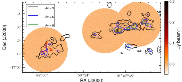
observations were obtained between 2012 July 8 and 2013 July 14. These data were observed as three fully sampled 30′ diameter circular regions using the PONG 1800 mode (Kackley et al. 2010). Each area of the sky was observed six times. Neighboring fields were set up to overlap slightly to create a more uniform noise in the final mosaic. Details for these observations are provided in Table 1, and the full IC 5146 region, observed at 850 μm, is shown in Figure1. Figures2and

3focus on the areas of 450 and 850 μm emission within Cocoon Nebula and the Northern Streamer, respectively.

The data reduction used for the maps presented here follows the GBS Legacy Release 1 methodology (GBS LR1) using the JCMT’s Starlink software (Currie et al. 2014),34which is discussed by Mairs et al. (2015). The data presented here were reduced using an iterative map-making technique (makemap in SMURF),35and gridded to 2″ pixels at 450 μm and 3″ pixels at 850 μm. The iterations were halted when the map pixels, on average, changed by <0.1% of the estimated map rms. These initial automask reductions of each individual scan were co-added to form a mosaic from which a signal-to-noise ratio (S/N) mask was produced for each region. The final external mask mosaic was produced from a second reduction using this S/N mask to define areas of emission. In IC 5146, the S/N mask included all pixels with S/Ns of 2 or higher at 850 μm. Testing by our data reduction team showed similar final maps using either an 850 μm-based or a 450 μm-based mask for the 450 μm reduction, when using the S/N-based masking scheme described Table 1

Noise Values within the SCUBA-2 Maps

Region Namea _R.A.b _Decl.b _s

850c s450c s850d s450d

(J2000.0) (J2000.0) (mJy arcsec−2_{) (mJy bm}−1₎

Coccon Nebula IC5146-H2 21:53:45 47:15:22 0.050 1.4 3.7 67

Northern Streamer IC5146-E 21:48:31 47:31:48 0.045 1.1 3.3 53

Northern Streamer IC5146-W 21:45:36 47:36:59 0.049 1.4 3.6 67

Notes.

a

Observation designation chosen by theGBS team, denoted as Target Name in the CADC database athttp://www3.cadc-ccda.hia-iha.nrc-cnrc.gc.ca/en/jcmt/. The Proposal ID for all these observations is MJLSG36.

b

Central position of each observation.

c

Pixel-to-pixel (rms) noise within each region after mosaicking together all observations.

d

Effective noise per beam (i.e., point source sensitivity) within each region after mosaicking together all observations.

34

Available athttp://starlink.eao.hawaii.edu/starlink.

35

SMURF is a software package used for reducing JCMT observations, and is described in more detail by Jenness et al. (2013) andChapin et al. (2013a,2013b).

here. Using identical masks at both wavelengths for the reduction ensures that the same large-scale filtering is applied to the observations at both wavelengths (e.g., maps of the ratio of flux densities at both wavelengths are less susceptible to differing large-scale flux recovery). Detection of emission structure and calibration accuracy are robust within the masked regions, but are less certain outside of the mask (Mairs et al. 2015).

Larger-scale structures are the most poorly recovered outside of the masked areas, while point sources are better recovered. A spatial filter of 600″ is used during both the automask and external mask reductions, and an additional filter of 200″ is applied during the final iteration of both reductions to the areas outside of the mask. Further testing by our data reduction team found that for 600″ filtering, flux recovery is robust for sources with a Gaussian FWHM ofless than 2 5, provided the mask is sufficiently large. Sources between 2 5 and 7 5 in diameter were detected, but both the flux density and the size were underestimated because Fourier components representing scales greater than 5′ were removed by the filtering process. Detection of sources larger than 7 5 is dependent on the mask used for reduction.

The data are calibrated in mJy per square arcsecond using aperture flux conversion factors of 2.34 Jy/pW/arcsec 2

0.08 Jy/pw/arcsec2 _{and 4.71 Jy/pW/arcsec  0.5}2 _Jy/pw/

arcsec2 at 850 μm and 450 μm, respectively, as derived from average values of JCMT calibrators (Dempsey et al.2013). The PONG scan pattern leads to lower noise in the map center and mosaic overlap regions, while data reduction and emission artifacts can lead to small variations in the noise over the whole map. The pointing accuracy of the JCMT is smaller than the pixel sizes we adopt, with current rms pointing errors of 1 2 in azimuth and 1 6 in elevation (seehttp://www.eaobservatory. org/JCMT/telescope/pointing/pointing.html); JCMT pointing accuracy in the era of SCUBA is discussed by Di Francesco et al. (2008).

The observations for IC 5146 were taken in grade 2 (0.05<t225 GHz<0.08) weather, corresponding to 0.21< t850 mm <0.34 (Dempsey et al.2013), with a mean value plus standard deviation oft225 GHzof 0.063±0.006. At 850 μm, the

final noise level in the mosaic is 0.048 mJy arcsec−2 _{per 3}

″ pixel, corresponding to a point source sensitivity of 3.7 mJy per 14 6 beam. At 450 μm, the final noise level is 1.3 mJy arcsec−2_{per 2″ pixel, corresponding to a point source}

sensitivity of 62 mJy per 9 8 beam (see Table1for details by

individual region). The beam sizes quoted here are the effective beams determined by Dempsey et al. (2013), and account for the fact that the beam shape is well-represented by the sum of a Gaussian primary beam shape and a fainter, larger Gaussian secondary beam.

The SCUBA-2 450 and 850 μm observations were convolved to a common beam size and compared to estimate the temperature of the emitting dust (see Appendix A). A clump temperature of 15 K is adopted throughout the remainder of this paper based on these results. Given that the CO(J= -3 2) rotational line lies in the middle of the 850 μm bandpass (Johnstone et al.2003; Drabek et al.2012), an analysis was undertaken to determine the level of CO contamination for those limited areas of the mapwhere CO observations also exist (see AppendixB). The contamination results show that none of the bright 850 μm emission is contaminated by more than 10%. Thus, for the remainder of this paper we use the uncorrected 850 μm map to determine source properties. All of the data presented in this paper are publicly available athttps://doi.org/10.11570/17.0001.

Kramer et al. (2003)previously imaged parts of IC 5146 at the JCMT with SCUBA (Holland et al.1999)at both 450 and 850 μm, reducing the data using the SCUBA User Reduction Facility (SURF; Jenness et al. 2002) and correcting for atmospheric extinction and sky noise. The SCUBA mapped region is ∼14′×2 5 in size and includes parts of the Northern Streamer, focusing on ridges. The authors find several peaks of high emission (corresponding to optical extinctions of >20 mag) in their maps that they attribute to dense prestellar structures and identify four clumps with high optical extinc-tions along ridges in the region. They construct a dust temperature map and conclude that there is a distribution of temperatures throughout the region, varying between 10 and 20 K, with an average of16.58 K, in agreement with the values determined in Appendix A. The temperatures of the cores tend toward the lower limit,Tc~12 K. Assuming this temperature and a dust emissivity ofk850= 0.01cm2g−1, their

derived core masses vary between 4M and 7M at their

adopted distance of 460 pc (these masses increase by about a factor of four at our adopted distance of 950 pc). The resolution of their maps was smoothed beyond the native JCMT resolution and so finer detail in the cloud structure was not analyzed. These original reductions are not directly available for comparison. The SCUBA Legacy Catalog reduction (Di Francesco et al. 2008)of the Northern Streamer, however, is available in the archive and was used to verify that the SCUBA-2 GBS data sets presented here are in broad agreement with the lower sensitivity Kramer et al. (2003)observations.

3.2. Extinction Map

Cambrésy (1999) first published an extinction map of the IC 5146 region using optical R-band star counts based on the comparison of local stellar densities (L. Cambrésy 1999). A more recent version of this IC 5146 extinction map (L. Cambrésy 2015, private communication) was derived using 2MASS near-infrared H-K data to measure stellar reddening that was then used to estimate the local extinction in the region following the technique described by Cambrésy et al. (2002). The spatial resolution of this unpublished map is 2′. Notably, known YSOs and foreground stars have not been removed during the map construction. Nevertheless, the quality and Figure 1. IC 5146 observed at 850 μm with SCUBA-2. Also shown are the

AV=3, 6, and 9 contours from the 2MASS-based extinction map (Section3.2). The Spitzer coverage of the region (Section 3.3)is almost identical to the SCUBA-2 coverage shown here.

resolution of this extinction map remain sufficent for the analysis required here. Figure 1 shows the AV=3, 6, and 9 contours from the extinction map overlaid on the dust continuum SCUBA-2 850 μm map.

3.3. Spitzer YSOs

The Spitzer Space Telescope observed the IC 5146 region (Harvey et al. 2008)using its InfraRed Array Camera (IRAC) and its Multiband Imaging Photometer for Spitzer (MIPS). The region observed by Spitzer is almost identical to the SCUBA-2 areal coverage shown in Figure 1. Over 200 candidate YSOs were identified in the region. Those sources with both IRAC and MIPS detections have been independently classified as Class 0+1, Flat, Class II, and Class III protostars by Dunham et al. (2015)as part of a larger analysis of YSOs throughout the entire Gould Belt. Dunham et al. (2015)determine YSO class through careful examination of the IR spectral energy distributions (SEDs) and their final catalog contains an analysis of contamination by background AGB stars, updated extinction corrections, and revised SEDs, improving upon previous

Spitzer YSO catalogs by Harvey et al. (2008) and Evans

et al. (2009).

The Spitzer survey results combined with the GBS SCUBA-2 continuum data sets are shown in Figures2and3. There are 131

Spitzer sources within the boundaries of the SCUBA-2

observations. Notably, the youngest YSOs, i.e., Class 0/I and Flat sources, are positioned near areas of dust emission, with few outliers whereas the older, Class II and III sources are more scattered.

4. Analysis

Near-infrared extinction maps (e.g., Cambrésy 1999) typi-cally trace the large-scale structure in a cloud complex while SCUBA-2 maps focus on denser, localized dust emission (e.g., Ward-Thompson et al.2016)and the identification of sources from the Spitzer survey traces the specific locations of YSOs (Dunham et al.2015). Considered together,these three diverse

data sets helpus to build a better model of how star formation is influenced at each scale.

4.1. Large-scale Structure

To investigate the connection between emission in the 850 μm SCUBA-2 map and the observed extinction, we restrict our continuum analysis to 850 μm pixels above an S/N of 3.5, which results in a cut of pixels below a value of 0.175 mJy arcsec−2_{. This threshold is chosen to prevent the}

total flux density measured being dominated by the noise from the large number of pixels with little signal. The extinction map, as introduced and discussed in Section 3.2, has a small number of zones with negative extinction caused by artifacts in the data set. We exclude these pixels from our extinction map analysis; noting that they make up only 6% of the total map area analyzed.

Under the assumption that the optical characteristics of the dust grains remain the same throughout IC 5146 and that the Figure 2. IC 5146 Cocoon Nebula. The left panel shows 850 μm dust continuum emission. The right panel shows 450 μm dust emission. Overlaid on the 850 μm map are contours denoting the boundaries of the clumps identified in this paper (Section4.2),while on the 450 μm map the locations of the Spitzer-classified YSOs, by type (see thelegend), are provided (Section4.3). In this region,there are 13 Class 0/I, 6 Flat, 65 Class II, and 9 Class III YSOs. The black star in the left panel shows the location of the B0 V Star BD+46° 3474 (Herbig & Reipurth2008).

Figure 3. IC 5146 Northern Streamer. Upper panel shows 850 μm dust continuum emission. Lower panel shows 450 μm dust emission. Overlaid on the 850 μm map are contours denoting the boundaries of the clumps identified in this paper (Section4.2)while on the 450 μm map the locations of the YSOs, by type (see legend), are provided (Section4.3). In this region there are 15 Class 0/I, 4 Flat, 14 Class II, and 6 Class III YSOs.

temperature of the dust is constant, the mass revealed by the 850 μm map is directly proportional to the integrated flux density. Following Hildebrand (1983), the submillimeter-derived mass, M850is k = M S d B Td , 1 850 850 2 850 850( ) ( ) where d is the distance to the cloud, S850,k850, and B850are the

integrated flux density, opacity, and Planck function measured at 850 μm respectively, and Td is the dust temperature. The opacity of the dust is quite uncertain and a source of significant on-going research. Following the GBS standard (Pattle et al. 2015; Rumble et al. 2015, 2016; Salji et al. 2015a,

2015b; Kirk et al.2016a,2016b; Lane et al.2016; Mairs et al.

2016), we adopt k850= 0.0125cm2g−1. Taking a fiducial

value for the temperature from Appendix A, Td=15 K

(consistent with that used by Kramer et al. 2003), and

assuming a distance to IC 5146, d =950 pc (Harvey

et al.2008), Equation (1)becomes ⎛ ⎝ ⎜ ⎞ ⎠ ⎟⎛ ⎝ ⎜ ⎞ ⎠ ⎟ ⎛ ⎝ ⎜ ⎞ ⎠ ⎟ ⎡ ⎣ ⎢ ⎢ ⎢ ⎤ ⎦ ⎥ ⎥ ⎥ k = ´ - M S d M 11.3 Jy 950 pc 0.0125 cm g exp 1 exp 1 . 2 T 850 850 2 850 2 1 1 17 K 17 K 15 K d

( )

( )

Note that decreasing the fiducial dust temperature to 10 K would raise the derived masses by about a factor of two.

The extinction map can also be used to derive masses assuming a linear relation between extinction and column density. We adopt the Savage & Mathis (1979) ratio of

= ´

NH AV 1.87 1021 cm−2mag−1 and assume a mean

molecular weightm = 2.37 (Kauffmann et al.2008).

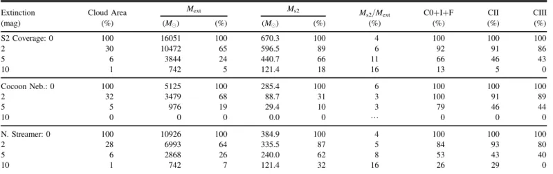
In Figure4, we show the cumulative fraction of mass within IC 5146 as a function of minimum extinction cut-off. The orange curve plots the mass derived from the extinction map using only the footprint of the SCUBA-2 observations. This curve reveals that most of the mass within the cloud lies at low extinction, with 50% of the mass below an extinction of AV=3. Alternatively, the blue curve plots the mass derived from the SCUBA-2 850 μm map (Equation (2)), assuming that the flux density is a direct linear proxy for column density. The cumulative curve clearly shows that the SCUBA-2 flux predominantly traces the higher extinction regions within the cloud, with 85% of the mass derived from the submillimeter continuum residing at an extinction greater than AV=3 and 50% of the mass at an extinction greater than AV=6. This result is similar to those found for other star-forming regions (e.g., Onishi et al. 1998; Johnstone et al. 2004; Hatchell et al.2005; Enoch et al.2006,2007; Kirk et al.2006; Könyves et al. 2013). Namely, the compact submillimeter emission within IC 5146 is intrinsically linked and heavily biased to regions of high dust column.

In total, we obtain a submillimeter-derived mass of~670M

for the IC 5146 region, above the S/N=3.5 cut-off. Taking only the extinction-derived mass coincident with the SCUBA-2

coverage, we obtain a mass of 16,000M and a mean

extinction of AV=1.7. This latter mass is about four times the CO mass estimate derived by Dobashi et al. (1992,1993). The discrepancy between the CO-derived mass and the

extinction-derived mass suggests one or both of the following situations: that a fraction of the extinction toward IC 5146 is unassociated with the cloud itself, and thus the extinction mass is somewhat over-estimated, or that the CO observations were not sensitive to the extended low AVemission from IC 5146, which is suggested by the comparison of the12_{CO and}13_CO

images presented by Dobashi et al. (1992). The extinction mass corresponds to roughly 24 times the submillimeter-derived mass. At AV >10, we find120M in the submillimeter map

and~740M in the extinction map. Breaking down the mass

estimates by sub-region within IC 5146, we find that the extinction-derived mass coincident with the single SCUBA-2 map covering the Cocoon Nebula is 5100M, or about

one-third of the entire mass for the IC 5146 region. The submillimeter-derived mass for this same region is 285M,

or just over 40% of the dense gas and dust in all of IC 5146. For the Northern Streamer, the extinction-derived mass coincident

with the two SCUBA-2 PONGs is ~104M_{, whereas the}

submillimeter-derived mass is 385M. Table 2 presents a

breakdown of the extinction-derived mass, submillimeter-derived mass, and YSO count as a function of AV threshold and sub-region.

4.2. Submillimeter Clumps

We used the FellWalker algorithm (Berry2015), part of the CUPID package (Berry et al. 2007, 2013) in Starlink, to identify notable structures in the 850 μm dust continuum map from SCUBA-2. The FellWalker technique searches for sets of disjoint clumps, each containing a single significant peak, using a gradient-tracing scheme. The algorithm is qualitatively similar to the better known Clumpfind (Williams et al. 1994) method that has been used extensively. The Fellwalker method, Figure 4. Cumulative mass as a function of extinction. The orange line plots the extinction-derived mass from the Cambrésy extinction map restricted to the SCUBA-2 areal coverage. The blue line plots the distribution of the submillimeter-derived mass from the 850 μm SCUBA-2 map, as a function of the coincident Cambrésy extinction. The colored dash lines show the cumulative distributions of the YSOs, by Class, as a function of the coincident Cambrésy extinction.

however, is more stable against noise and less susceptible to small changes in the input parameters (Watson 2010).

We ran FellWalker with several parameters changed from the default recommended values to achieve two goals: to recover faint but visually distinct objects missed with the default settings and to subdivide several larger structures that had visually apparent substructure not captured with the default settings. Table 3 lists the non-default parameters we adopted. Note that FellWalker assumes a single global noise value for its calculations, while our observations have some variation in noise level: the center of each PONG is about 20% less noisy than the typical rms, and in the Streamer, the overlap area between the two neighboring PONGS is about 25% less noisy, while the edges of the mosaic have a higher noise level than the typical rms. This observational fact informs our two-part clump-identification strategy: we first identify candidate clumps using FellWalker criteria that are generally more relaxed than the default values, and then run an independent program to cull this candidate clump list to ensure that all sources satisfy the same local S/N criteria. To achieve our first goal of recovering faint but visually distinct objects, we lowered the minimum flux density value allowed in clump pixels below the default value (see the “Noise” parameter in Table3). Allowing fainter pixels to be associated with clumps also led to the identification of some spurious noise features as clumps. We eliminated these false positive clumps through the use of an automated procedure wherein each clump was required to have 10 or more pixels with a local S/N value of 3.5 or higher. (Note that clumps passing this test are allowed to contain additional pixels with lower local S/N values.) This automated procedure reduced the initial FellWalker catalog from 273 clump candidates to 96 reliable clumps. All of these 96 reliable clumps also passed a visual inspection. We note that the vast majority of these clumps also have a good correspondence to the clump catalog obtained using the default FellWalker settings. Namely, about 10% of the clumps in our catalog were either subdivided less or were not identified using the default settings.

Table 4 reports the observed properties of the 96 reliable clumps, including the peak flux densities F850 and F450 in

Jy bm−1

, the total integrated flux density at 850 μm within the clump boundary S850in Jy, and the areal extent of each clump A

in arcsec2. As noted in Section 3.1, the SCUBA-2 850 μm

bandpass straddles the CO(J= -3 2) rotational line that can result in CO contamination of the continuum flux. Where possible, the peak and total flux density at 850 μm associated with each clump have been investigated for possible CO contamination (AppendixB)and in all cases the contamination values are found to be less than 10%. The results shown are not corrected for CO contamination.

Table 5 presents the derived properties of the clumps. The effective radius of each clump, RC in pc, is derived through equating the area within the clump boundary with that of a circular aperture. The masses of the clumps are computed using Equation (2)under the assumption thatTd=15 K(Section3.1 and Appendix A). Decreasing the dust temperature to 10 K raises the derived masses by about a factor of two. The masses span a range from 0.5M to 116 M , the mean clump mass is

8M , and the median clump mass is 3.7 M . The total mass in

clumps is ~750M, slightly larger than the

submillimeter-derived mass found in the previous section. This difference is because we allow the clump boundaries to include not only the bright central emission, but also extended more diffuse emission (below a local S/N=3.5 level) that is clearly associated. In our analysis in Section4.1, we use a conservative global S/N=3.5

threshold to prevent noise spikes at lower S/N levels from being included in our results. Since most of the area of our map appears to lack real emission, noise spikes would make a significant contribution to flux measured at levels below an S/N of 3.5.

Table 2

Cumulative Mass above Different Extinction Thresholds

Extinction Cloud Area Mext Ms2 _{Ms2/Mext C0+I+F CII CIII}

(mag) (%) (M )_ (%) (M )_ (%) (%) (%) (%) (%) S2 Coverage: 0 100 16051 100 670.3 100 4 100 100 100 2 30 10472 65 596.5 89 6 92 91 86 5 6 3844 24 440.7 66 11 66 46 43 10 1 742 5 121.4 18 16 13 5 0 Cocoon Neb.: 0 100 5125 100 285.4 100 6 100 100 100 2 32 3479 68 88.7 31 3 100 91 89 5 5 976 19 29.4 10 3 79 46 44 10 0 0 0 0.0 0 L 0 0 0 N. Streamer: 0 100 10926 100 384.9 100 4 100 100 100 2 28 6993 64 335.5 87 5 84 93 80 5 6 2868 26 240.0 62 8 53 43 40 10 1 742 7 121.4 32 16 26 29 0 Table 3 FellWalker Parameters

Name Descriptor Value

AllowEdge exclude clumps touching the noisier map edge 0.00

CleanIter smooth clump edges 15.0

rms as measured in the map 0.05

FlatSlope increase the gradient required for associating pixels with a peak

2.0*rms MinDip reduce the difference between peaks required to

have multiple objects

1.5*rms MaxJump reduce the search radius to combine peaks into a

single object

2.0 MinPix minimum number of pixels per clump 10.0 Noise allow fainter pixels to be associated with a peak 0.35*rms

Table 4 Identified 850 μm Clumps

Clumpa Source Nameb R.A.c Decl.c Peak Fluxd Peak Fluxd Total Fluxd Aread

Number (MJLSG...) (J2000.0) (J2000.0) F850(Jy/Bm) F450(Jy/Bm) S850(Jy) A (arcsec2)

1 J214428.6+473616 21:44:28.57 47:36:15.80 0.05 0.46 0.16 2457 2 J214439.4+474416 21:44:39.35 47:44:16.02 0.07 0.47 0.14 2151 3 J214439.4+473522 21:44:39.40 47:35:22.03 0.05 0.48 0.09 1305 4 J214442.8+474641 21:44:42.80 47:46:41.03 0.36 1.54 0.92 5292 5 J214443.6+474532 21:44:43.59 47:45:32.27 0.08 0.52 0.32 3051 6 J214448.1+474458 21:44:48.15 47:44:57.60 0.09 0.49 0.31 3573 7 J214448.9+473649 21:44:48.93 47:36:48.82 0.07 0.46 0.27 3168 8 J214452.2+474032 21:44:52.16 47:40:31.76 0.41 1.62 2.10 8163 9 J214454.3+474214 21:44:54.25 47:42:14.36 0.06 0.40 0.08 990 10 J214454.8+473903 21:44:54.79 47:39:02.51 0.08 0.45 0.07 693 11 J214455.6+473927 21:44:55.61 47:39:26.75 0.16 0.65 0.42 1836 12 J214458.2+474154 21:44:58.17 47:41:54.48 0.19 0.67 0.56 3258 13 J214458.2+474003 21:44:58.18 47:40:03.48 0.16 0.69 1.44 5832 14 J214458.8+473434 21:44:58.80 47:34:33.65 0.08 0.51 0.16 1566 15 J214459.7+473937 21:44:59.74 47:39:36.92 0.10 0.52 0.15 1332 16 J214460.7+473355 21:44:60.68 47:33:55.18 0.08 0.69 0.29 2340 17 J214462.9+473302 21:44:62.90 47:33:01.81 0.12 0.64 0.37 2574 18 J214506.5+474357 21:45:06.45 47:43:56.82 0.10 0.49 0.51 5184 19 J214507.5+473345 21:45:07.53 47:33:45.11 0.08 0.54 0.20 1719 20 J214507.7+473809 21:45:07.70 47:38:09.17 0.08 0.52 0.24 2493 21 J214508.2+473306 21:45:08.22 47:33:06.31 0.43 2.01 1.25 5562 22 J214512.9+473723 21:45:12.87 47:37:22.60 0.07 0.50 0.27 2601 23 J214513.3+473235 21:45:13.34 47:32:34.73 0.09 0.55 0.34 3033 24 J214514.1+473705 21:45:14.10 47:37:04.95 0.07 0.46 0.10 1368 25 J214527.7+473545 21:45:27.66 47:35:44.64 0.11 0.50 0.28 2241 26 J214531.1+473616 21:45:31.14 47:36:15.57 0.10 0.61 0.52 3636 27 J214535.4+473541 21:45:35.38 47:35:40.70 0.11 0.67 0.60 3789 28 J214550.8+473736 21:45:50.81 47:37:35.72 0.06 0.43 0.16 2061 29 J214552.3+473745 21:45:52.27 47:37:45.10 0.07 0.45 0.11 1512 30 J214558.8+473602 21:45:58.75 47:36:01.74 0.17 0.74 0.98 5940 31 J214561.5+473550 21:45:61.45 47:35:50.42 0.12 0.45 0.32 2511 32 J214617.8+473345 21:46:17.75 47:33:45.43 0.07 0.53 0.12 1305 33 J214620.4+473407 21:46:20.37 47:34:07.06 0.08 0.61 0.34 3771 34 J214632.8+473355 21:46:32.84 47:33:55.02 0.06 0.65 0.26 3591 35 J214649.8+473314 21:46:49.82 47:33:13.90 0.07 0.46 0.38 4311 36 J214650.0+473429 21:46:49.96 47:34:28.93 0.08 0.41 0.45 4536 37 J214651.3+473953 21:46:51.33 47:39:53.24 0.07 0.44 0.33 4500 38 J214656.9+473312 21:46:56.94 47:33:12.48 0.06 0.38 0.28 3438 39 J214660.2+473949 21:46:60.24 47:39:49.21 0.07 0.33 0.11 1206 40 J214704.4+473241 21:47:04.41 47:32:41.12 0.10 0.45 0.18 1125 41 J214706.2+473936 21:47:06.21 47:39:35.50 0.12 0.45 0.77 5472 42 J214706.4+473306 21:47:06.43 47:33:05.55 0.14 0.51 1.35 10863 43 J214708.9+473157 21:47:08.95 47:31:57.09 0.06 0.37 0.24 2592 44 J214709.2+473933 21:47:09.19 47:39:33.14 0.09 0.44 0.62 5139 45 J214720.5+473433 21:47:20.48 47:34:32.52 0.05 0.39 0.09 1152 46 J214722.7+473342 21:47:22.66 47:33:41.97 0.16 0.60 0.78 3996 47 J214722.8+473212 21:47:22.84 47:32:12.01 0.70 2.92 10.34 21312 48 J214724.8+473103 21:47:24.75 47:31:03.40 0.19 0.63 0.72 3204 49 J214724.8+473815 21:47:24.78 47:38:15.41 0.07 0.40 0.26 3105 50 J214726.6+473534 21:47:26.58 47:35:33.78 0.06 0.31 0.12 1566 51 J214729.0+473734 21:47:29.01 47:37:34.28 0.06 0.39 0.18 2304 52 J214730.3+473202 21:47:30.26 47:32:01.53 0.19 0.67 0.92 4275 53 J214730.6+472935 21:47:30.55 47:29:34.59 0.07 0.38 0.21 2556 54 J214733.5+473944 21:47:33.51 47:39:44.18 0.05 0.42 0.05 837 55 J214750.6+473751 21:47:50.64 47:37:50.54 0.08 0.44 0.28 3024 56 J214753.9+473736 21:47:53.93 47:37:36.16 0.07 0.50 0.33 2880 57 J214759.1+473625 21:47:59.11 47:36:25.14 0.29 1.48 1.11 6426 58 J214812.8+473625 21:48:12.75 47:36:24.63 0.07 0.42 0.24 2862 59 J214842.8+472560 21:48:42.81 47:25:59.77 0.07 0.35 0.08 1044 60 J214846.1+472551 21:48:46.07 47:25:51.30 0.08 0.44 0.38 3150 61 J214846.1+472515 21:48:46.13 47:25:15.31 0.10 0.47 0.37 2943 62 J214852.0+473134 21:48:52.05 47:31:34.26 0.11 0.50 0.64 5553 63 J214854.8+472723 21:48:54.80 47:27:22.69 0.05 0.39 0.11 1647

Figures2 and3use contours to show the clump boundaries within the two IC 5146 molecular cloud regions. Within the Cocoon Nebula, the majority of the clumps merge together to create a broken ring around the central star cluster while in the Northern Streamer, the clumps fan out along the known filaments uncovered by Herschel (Arzoumanian et al.2011). In both regions, however, the distribution of clumps typically generate one-dimensional sequences and relatively straight filamentary chains.

Although the single most massive clump lies in the Northern Streamer, the typical clump in the Cocoon Nebula is about twice as massive (mean 11.5M , median 6.6 M ) as that found

in the Northern Streamer (mean 6.5M , median 3.2 M ),

assuming that the temperatures and dust properties are the same across all of IC 5146. Many of the clumps in IC 5146 are closely related to the YSOs, especially the Class 0 and I sources (see Section4.3). Of the 70 clumps in the Northern Streamer

(_{Clumps 1–70 in Table} 4), 15 (21%) have at least one

associated YSO. In contrast, of the 26 clumps observed in the Cocoon Nebula (Clumps 71–96), 14 (54%) harbour at least one

YSO within theirboundaries. At first glance, this suggests that star formation is more active in the Cocoon Nebula. It is also possible, however, that the earliest stage of star (clump) formation is ramping down in the Cocoon Nebula and therefore the majority of the remaining clumps are presently star-forming. In the Northern Streamer, a smaller fraction of clumps host embedded YSOs and almost all of the YSOs in the region are still heavily embedded in the dust continuum, implying an earlier evolutionary time (see also Section4.3).

Although these clumps are likely to have additional non-thermal support, given their large size and mass, it is interesting to compare them against known static isothermal models, such as Bonnor–Ebert (BE) spheres (Ebert1955; Bonnor1956). BE sphere models denote a continuum of solutions for equilibrium self-gravitating isothermal spheres with external bounding pressure, from very-low-mass objects that have an almost constant density throughout to critical models that are on the very edge of gravitational collapse and have a large variation in density between the center and the edge. This continuum of models can be represented by a single observational measure, Table 4

(Continued)

Clumpa _{Source Name}b _R.A.c _Decl.c _{Peak Flux}d _{Peak Flux}d _{Total Flux}d _Aread

Number (MJLSG...) (J2000.0) (J2000.0) F850(Jy/Bm) F450(Jy/Bm) S850(Jy) A (arcsec2)

64 J214856.3+473026 21:48:56.30 47:30:25.93 0.17 0.68 0.72 5112 65 J214923.5+472406 21:49:23.47 47:24:05.95 0.05 0.42 0.05 666 66 J214924.3+472851 21:49:24.26 47:28:51.06 0.27 0.94 1.43 7146 67 J214931.0+472607 21:49:30.99 47:26:06.99 0.07 0.49 0.25 2979 68 J214931.5+472725 21:49:31.48 47:27:25.06 0.14 0.66 0.74 3996 69 J214933.9+472710 21:49:33.86 47:27:10.39 0.18 0.71 0.65 3114 70 J214936.8+472711 21:49:36.82 47:27:10.78 0.10 0.49 0.27 1971 71 J215235.8+471314 21:52:35.75 47:13:13.99 0.05 0.47 0.12 1638 72 J215238.4+471438 21:52:38.38 47:14:38.08 0.18 0.96 0.58 4833 73 J215307.0+471521 21:53:06.95 47:15:20.85 0.17 0.67 1.76 7785 74 J215307.3+471424 21:53:07.25 47:14:23.86 0.12 0.65 0.39 2367 75 J215312.6+471457 21:53:12.55 47:14:56.95 0.21 0.84 2.38 8775 76 J215312.9+471136 21:53:12.87 47:11:35.96 0.06 0.45 0.17 2655 77 J215314.6+471621 21:53:14.60 47:16:20.99 0.18 0.73 2.05 9630 78 J215315.5+471821 21:53:15.46 47:18:21.00 0.08 0.54 0.39 3654 79 J215317.8+471939 21:53:17.81 47:19:39.03 0.11 0.65 1.17 7893 80 J215324.6+471730 21:53:24.61 47:17:30.11 0.08 0.50 0.24 2466 81 J215331.4+472203 21:53:31.38 47:22:03.17 0.17 0.91 1.59 7974 82 J215333.2+471415 21:53:33.17 47:14:15.18 0.24 0.86 1.46 6156 83 J215334.6+472057 21:53:34.63 47:20:57.18 0.18 0.80 2.66 9783 84 J215335.5+471727 21:53:35.52 47:17:27.19 0.16 0.67 0.55 2088 85 J215336.4+471506 21:53:36.41 47:15:06.19 0.07 0.45 0.23 1908 86 J215336.7+471903 21:53:36.70 47:19:03.19 0.32 1.29 1.33 5175 87 J215336.7+471415 21:53:36.71 47:14:15.19 0.10 0.71 0.30 2358 88 J215337.3+471736 21:53:37.29 47:17:36.19 0.14 0.63 1.12 4509 89 J215337.6+471948 21:53:37.58 47:19:48.19 0.31 1.16 1.82 6129 90 J215340.8+471527 21:53:40.83 47:15:27.20 0.05 0.43 0.17 2259 91 J215345.3+471357 21:53:45.25 47:13:57.20 0.05 0.50 0.10 1485 92 J215345.8+471736 21:53:45.84 47:17:36.20 0.10 0.60 0.49 3357 93 J215350.5+471233 21:53:50.55 47:12:33.18 0.10 0.69 0.91 6192 94 J215350.5+471348 21:53:50.55 47:13:48.18 0.21 0.94 1.74 5652 95 J215354.7+471321 21:53:54.67 47:13:21.16 0.21 0.95 1.51 5445 96 J215355.9+471354 21:53:55.85 47:13:54.15 0.20 0.91 1.39 6354 Notes. a

Clump observation designation.

b

The source name is based on the coordinates of the peak emission location of each object in R.A. and decl.: Jhhmmss.s±ddmmss.

c

Peak position, at 850 μm, for each clump.

d

Table 5

Derived Properties of the Identified 850 μm Clumps Clumpa _{Total Mass}b _{Jeans Mass}b _{Clump Radius}b _{Concentration}b _{Total YSOs}

Class0+I/Flat Class II/III Class0+I/Flat Number M850(Me) MJ(Me) Rc(parsec) Containedc Containedc Near Peakc Near Peakc

1 1.77 5.24 0.13 0.71 0 0 0 0 2 1.60 4.91 0.12 0.78 0 0 0 0 3 0.98 3.82 0.09 0.68 0 0 0 0 4 10.40 7.70 0.19 0.88 2 1 0 1 5 3.65 5.84 0.14 0.69 0 0 0 0 6 3.50 6.32 0.16 0.76 1 1 0 1 7 3.08 5.95 0.15 0.70 0 0 0 0 8 23.67 9.56 0.23 0.85 3 2 0 2 9 0.95 3.33 0.08 0.64 0 0 0 0 10 0.75 2.79 0.07 0.72 0 0 0 0 11 4.71 4.53 0.11 0.66 0 0 0 0 12 6.26 6.04 0.15 0.78 1 1 0 1 13 16.21 8.08 0.20 0.63 0 0 0 0 14 1.77 4.19 0.10 0.71 0 0 0 0 15 1.71 3.86 0.09 0.74 0 0 0 0 16 3.25 5.12 0.13 0.63 0 0 0 0 17 4.17 5.37 0.13 0.72 1 1 0 1 18 5.69 7.62 0.19 0.76 0 0 0 0 19 2.27 4.39 0.11 0.65 0 0 0 0 20 2.73 5.28 0.13 0.69 0 0 0 0 21 14.10 7.89 0.19 0.88 1 1 0 1 22 3.00 5.40 0.13 0.64 0 0 0 0 23 3.85 5.83 0.14 0.70 0 0 0 0 24 1.15 3.91 0.10 0.73 0 0 0 0 25 3.14 5.01 0.12 0.72 0 0 0 0 26 5.79 6.38 0.16 0.67 1 1 0 1 27 6.72 6.51 0.16 0.67 0 0 0 0 28 1.81 4.80 0.12 0.69 0 0 0 0 29 1.21 4.11 0.10 0.74 0 0 0 0 30 11.05 8.15 0.20 0.76 1 1 0 1 31 3.64 5.30 0.13 0.75 0 0 0 0 32 1.38 3.82 0.09 0.67 0 0 0 0 33 3.86 6.50 0.16 0.72 0 0 0 0 34 2.92 6.34 0.16 0.72 0 0 0 0 35 4.28 6.95 0.17 0.70 0 0 0 0 36 5.11 7.13 0.18 0.71 0 0 0 0 37 3.68 7.10 0.17 0.76 0 0 0 0 38 3.21 6.20 0.15 0.69 0 0 0 0 39 1.24 3.67 0.09 0.70 0 0 0 0 40 2.01 3.55 0.09 0.64 0 0 0 0 41 8.67 7.83 0.19 0.71 1 1 0 1 42 15.20 11.03 0.27 0.78 1 1 0 0 43 2.72 5.39 0.13 0.64 1 0 0 0 44 6.96 7.58 0.19 0.67 0 0 0 0 45 1.05 3.59 0.09 0.61 0 0 0 0 46 8.78 6.69 0.16 0.71 0 0 0 0 47 116.36 15.44 0.38 0.83 5 4 0 2 48 8.15 5.99 0.15 0.71 0 0 0 0 49 2.94 5.90 0.14 0.69 0 0 0 0 50 1.32 4.19 0.10 0.71 0 0 0 0 51 1.99 5.08 0.12 0.71 0 0 0 0 52 10.31 6.92 0.17 0.73 2 0 0 0 53 2.35 5.35 0.13 0.70 0 0 0 0 54 0.61 3.06 0.08 0.71 0 0 0 0 55 3.13 5.82 0.14 0.73 0 0 0 0 56 3.69 5.68 0.14 0.63 1 1 0 0 57 12.51 8.48 0.21 0.85 1 1 0 1 58 2.66 5.66 0.14 0.71 0 0 0 0 59 0.88 3.42 0.08 0.74 0 0 0 0 60 4.29 5.94 0.15 0.65 0 0 0 0 61 4.16 5.74 0.14 0.71 0 0 0 0 62 7.23 7.88 0.19 0.75 0 0 0 0 63 1.19 4.29 0.11 0.70 0 0 0 0

the concentration parameter, as described by Johnstone et al. (2000)and Kirk et al. (2006):

⎛ ⎝ ⎜ ⎞ ⎠ ⎟⎛ ⎝ ⎜ ⎞ ⎠ ⎟ = -C B A S F 1 1.13 , 3 2 850 850 ( )

where B=14. 6 is the effective 850 mm JCMT beamsize

(Dempsey et al. 2013). To be stable against collapse,

isothermal clumps with concentrations above 0.72 require additional support mechanisms such as pressure from magnetic fields. The concentration for each of the clumps in IC 5146 is included in Table 5. The concentrations range from 0.58 to 0.88, with a mean value of 0.70. Thus, the typical submillimeter clump appears on the verge of gravo-thermal instability based on concentration. It is worth noting that this analysis does not depend on the inferred temperature or dust emissivity (see Equation (3)) but does require that these properties remain constant throughout the clump. Furthermore, the concentration parameter is sensitive to the derived radius of the clump and thus choosing lower surface brightness

thresholds for clump boundaries is likely to result in larger derived concentrations. As a result, individual concentration values should be treated with caution while the variations in concentration between clumps and across ensembles of clumps provides indications of the varying importance of gravity and non-thermal properties.

For all of the clumps in IC 5146, we also compare the derived mass, using Equation (2), against the maximum (Jeans-critical) mass of a stable thermally supported sphere of the same size Rc following the strategy of Sadavoy et al. (2010) and assuming a gas temperature of 15 K consistent with that determined from the dust

⎜ ⎟ ⎛ ⎝ ⎞ ⎠ ⎛ ⎝ ⎜ ⎞ ⎠ ⎟ =  M 29 T R M 15 K 0.07 pc . 4 J c ( )

As shown in Table 5, the range of Jeans masses, 2.7< <



M MJ 15.4, is significantly smaller than the range of

clump masses M850. Nevertheless, a majority of the observed

clumps appear to be Jeans stable according to this criterion: i.e., 62 of 96 or 65% have M850 MJ<1, with a noticeable Table 5

(Continued)

Clumpa Total Massb Jeans Massb Clump Radiusb Concentrationb Total YSOs Class0+I/Flat Class II/III Class0+I/Flat Number M850(Me) MJ(Me) Rc(parsec) Containedc Containedc Near Peakc Near Peakc

64 8.11 7.56 0.19 0.80 0 0 0 0 65 0.53 2.73 0.07 0.68 0 0 0 0 66 16.13 8.94 0.22 0.82 0 0 0 0 67 2.84 5.77 0.14 0.73 0 0 0 0 68 8.36 6.69 0.16 0.69 0 0 0 0 69 7.36 5.90 0.15 0.72 0 0 0 0 70 3.06 4.70 0.12 0.68 0 0 0 0 71 1.33 4.28 0.11 0.65 0 0 0 0 72 6.52 7.35 0.18 0.84 2 1 0 1 73 19.82 9.33 0.23 0.67 0 0 0 0 74 4.42 5.15 0.13 0.68 1 1 0 1 75 26.83 9.91 0.24 0.69 1 0 0 0 76 1.87 5.45 0.13 0.72 0 0 0 0 77 23.10 10.38 0.25 0.71 0 0 0 0 78 4.42 6.40 0.16 0.66 0 0 0 0 79 13.22 9.40 0.23 0.68 0 0 0 0 80 2.74 5.25 0.13 0.71 0 0 0 0 81 17.85 9.45 0.23 0.71 1 1 0 1 82 16.44 8.30 0.20 0.76 3 2 0 1 83 29.97 10.46 0.26 0.63 1 1 0 1 84 6.24 4.83 0.12 0.60 1 1 0 0 85 2.64 4.62 0.11 0.58 1 0 0 0 86 14.99 7.61 0.19 0.81 2 2 0 1 87 3.35 5.14 0.13 0.69 0 0 0 0 88 12.65 7.10 0.17 0.58 0 0 0 0 89 20.54 8.28 0.20 0.77 1 1 0 0 90 1.88 5.03 0.12 0.67 2 0 1 0 91 1.17 4.08 0.10 0.66 0 0 0 0 92 5.54 6.13 0.15 0.65 0 0 0 0 93 10.25 8.33 0.20 0.64 1 0 0 0 94 19.54 7.95 0.20 0.65 1 1 0 1 95 17.01 7.81 0.19 0.68 0 0 0 0 96 15.66 8.43 0.21 0.74 2 1 0 0 Notes. a

Clump observation designation.

b

See the text for definitions.

c

difference between the two regions. In the Northern Streamer, 51 of 70, or 73%, are stable by this criterion whereas in the Cocoon Nebula only 11 of 26, or 42%, appear to bestable. Furthermore, the subset of 29 clumps across IC 5146 harbour-ing embedded protostars show a propensity for instability, with 20 of 29, or 69%, having M850 MJ >1. The Jeans stability argument is extremely sensitive to the assumed temperature given that the Jeans mass increases and the dust continuum mass decreases with increasing temperature. Nevertheless, assuming that the properties of clumps are similar across IC 5146, the Jeans stability ratio (M850 MJ) allows for an ordering of the importance of self-gravity within clumps, with the highest ratios denoting the most gravitationally unstable clumps.

4.3. Dust Continuum and YSOs

Spitzerobserved the IC 5146 region (Harvey et al.2008)and identified 131 YSOs within the SCUBA-2 areal coverage, classified as either Class 0/I (28), Flat (10), Class II (79), or Class III (14) (Dunham et al.2015). Of these, 38 reside in the Northern Streamer, with 19 Class 0/I and Flat protostars versus 19 Class II+III more evolved YSOs. The Cocoon Nebula has 91 YSOs in total, divided into 19 Class 0/I and Flat protostars versus 74 Class II+IIIs. Tables6and7detail the location, the underlying 450 μm and 850 μm flux density, and the associated near-infrared extinction for Spitzer “protostars” (Class 0/I and Flat) and “evolved sources” (Class II+III), respectively. These tables also note the identifier of the clump in which each YSO resides as well as both the offset distance to the nearest clump Table 6

SpitzerProtostars: Flux and Extinction

YSO Indexa R.A.b Decl.b Class Typec F850d F450d AV

d

Hoste Neareste Distance

(J2000.0) (J2000.0) (Jy/Bm) (Jy/Bm) mag Clump Clump (arcsec)

1727 21:44:43.0 +47:46:43 0+I 0.323 0.99 3.72 4 4 2.8 1729 21:44:48.3 +47:44:59 0+I 0.059 0.39 5.41 6 6 2.1 1731 21:44:51.7 +47:40:44 0+I 0.119 0.34 7.28 8 8 13.1 1732 21:44:52.0 +47:40:30 0+I 0.386 1.41 7.43 8 8 2.4 1736 21:44:53.9 +47:45:43 0+I −0.002 0.20 4.00 L 6 73.7 1737 21:44:57.0 +47:41:52 FLAT 0.047 0.00 5.41 12 12 12.1 1739 21:45:02.6 +47:33:07 0+I 0.102 0.00 1.80 17 17 6.0 1741 21:45:08.3 +47:33:05 FLAT 0.435 1.83 4.18 21 21 1.5 1742 21:45:27.8 +47:45:50 0+I −0.019 −0.14 1.74 L 18 243.4 1743 21:45:31.2 +47:36:21 0+I 0.081 −0.07 1.63 26 26 5.5 1746 21:45:58.5 +47:36:01 0+I 0.126 0.31 14.23 30 30 2.6 1753 21:47:03.0 +47:33:14 0+I 0.034 0.16 8.70 42 42 35.8 1754 21:47:06.0 +47:39:39 0+I 0.074 0.34 4.22 41 41 4.1 1757 21:47:21.2 +47:32:26 FLAT 0.299 0.84 13.65 47 47 21.7 1758 21:47:22.6 +47:32:05 0+I 0.530 1.86 13.65 47 47 7.4 1759 21:47:22.7 +47:32:14 0+I 0.662 2.74 13.65 47 47 2.4 1760 21:47:28.7 +47:32:17 FLAT 0.124 0.46 11.47 47 52 22.1 1763 21:47:55.6 +47:37:11 0+I 0.046 0.10 4.45 56 56 30.3 1764 21:47:59.2 +47:36:26 0+I 0.246 1.22 3.54 57 57 1.3 1765 21:52:14.3 +47:14:54 0+I 0.004 −0.14 3.31 L 71 240.3 1776 21:52:37.7 +47:14:38 0+I 0.161 0.55 6.19 72 72 6.9 1788 21:53:06.9 +47:14:34 0+I 0.094 0.38 5.23 74 74 10.7 1798 21:53:25.0 +47:16:22 FLAT 0.004 0.10 5.22 L 80 68.2 1803 21:53:28.3 +47:15:43 0+I −0.008 −0.04 5.52 L 85 90.4 1804 21:53:28.6 +47:15:51 0+I 0.003 0.18 5.52 L 85 91.3 1811 21:53:30.4 +47:13:10 FLAT −0.002 0.18 5.02 L 82 71.0 1814 21:53:31.4 +47:22:17 0+I 0.088 0.34 4.26 81 81 13.8 1818 21:53:33.0 +47:14:39 FLAT 0.015 0.13 5.95 82 82 23.9 1820 21:53:33.1 +47:14:18 0+I 0.212 0.46 6.00 82 82 2.9 1823 21:53:33.9 +47:17:24 0+I 0.063 0.12 5.79 84 84 16.8 1826 21:53:34.7 +47:20:44 FLAT 0.173 0.68 5.06 83 83 13.2 1830 21:53:36.3 +47:19:03 0+I 0.243 0.62 6.08 86 86 4.1 1831 21:53:37.0 +47:18:17 0+I 0.039 −0.10 5.77 86 88 40.9 1833 21:53:38.3 +47:19:35 FLAT 0.229 0.67 5.94 89 89 15.1 1841 21:53:42.0 +47:14:26 FLAT 0.010 −0.10 6.72 L 91 43.9 1846 21:53:49.7 +47:13:51 0+I 0.135 0.24 7.20 94 94 9.1 1849 21:53:55.7 +47:20:30 0+I 0.019 −0.22 2.50 L 89 188.8 1851 21:53:58.1 +47:14:45 0+I 0.014 0.11 4.63 96 96 55.8 Notes. a

YSO observation designation from Dunham et al. (2015).

b

Location of YSO.

c

YSO Class (see the text).

d

See text for definitions.

e

Table 7

SpitzerEvolved Sources: Flux and Extinction

YSO Indexa R.A.b Decl.b Class Typec F850d F450d AV

d

Hoste Neareste Distance

(J2000.0) (J2000.0) (Jy/Bm) (Jy/Bm) mag Clump Clump (arcsec)

1728 21:44:44.4 +47:46:49 II 0.070 0.08 3.72 4 4 18.0 1730 21:44:49.1 +47:46:21 II 0.003 −0.09 4.07 L 4 66.7 1733 21:44:52.3 +47:44:55 II −0.009 0.06 3.85 L 6 42.0 1734 21:44:53.2 +47:46:07 II 0.004 −0.05 3.37 L 6 86.1 1735 21:44:53.4 +47:40:48 II 0.064 0.20 7.50 8 8 20.5 1738 21:45:01.5 +47:41:22 III 0.007 0.22 6.23 L 12 46.8 1740 21:45:02.9 +47:42:29 III 0.009 −0.21 4.49 L 12 58.9 1744 21:45:41.0 +47:37:07 II −0.014 −0.00 3.81 L 28 103.3 1745 21:45:57.1 +47:19:31 II −0.020 0.01 2.35 L 32 880.0 1747 21:46:05.7 +47:20:48 II −0.004 −0.14 1.01 L 32 787.2 1748 21:46:22.0 +47:35:00 III −0.009 −0.29 8.04 L 33 55.5 1749 21:46:26.6 +47:44:15 II −0.006 0.05 2.15 L 37 361.9 1750 21:46:41.3 +47:34:31 II −0.007 −0.06 5.86 L 36 87.7 1751 21:46:46.7 +47:35:55 III −0.019 −0.08 3.31 L 36 92.2 1752 21:46:49.2 +47:45:08 III −0.003 0.33 1.49 L 37 315.6 1755 21:47:10.8 +47:32:04 II 0.022 −0.05 14.19 43 43 20.0 1756 21:47:20.6 +47:32:03 II 0.381 1.33 13.65 47 47 24.4 1761 21:47:32.9 +47:32:08 II 0.041 0.12 10.98 52 52 27.5 1762 21:47:34.2 +47:32:05 II 0.016 −0.22 10.98 52 52 40.0 1766 21:52:19.2 +47:15:55 II 0.004 −0.02 4.15 L 72 209.8 1767 21:52:19.6 +47:14:38 II −0.007 0.11 3.05 L 71 184.8 1768 21:52:30.7 +47:14:06 II −0.000 −0.01 4.22 L 71 73.2 1769 21:52:32.6 +47:13:46 II −0.005 0.17 4.15 L 71 45.4 1770 21:52:32.7 +47:14:09 II −0.011 −0.03 4.15 L 71 63.2 1771 21:52:33.2 +47:10:50 II 0.008 −0.12 1.64 L 71 146.3 1772 21:52:34.0 +47:13:43 II 0.042 −0.56 4.02 L 71 34.1 1773 21:52:34.5 +47:14:40 II 0.005 0.31 5.31 L 72 39.5 1774 21:52:36.1 +47:11:56 II 0.003 −0.23 2.62 L 71 78.1 1775 21:52:36.5 +47:14:36 II 0.001 −0.11 6.19 72 72 19.2 1777 21:52:39.7 +47:11:10 III −0.017 −0.04 2.77 L 71 130.3 1778 21:52:41.2 +47:12:52 II 0.021 −0.17 4.21 L 71 59.7 1779 21:52:42.7 +47:12:09 II −0.001 0.17 3.86 L 71 96.1 1780 21:52:42.7 +47:10:13 II −0.019 0.12 2.14 L 71 194.3 1781 21:52:45.4 +47:10:39 III −0.002 0.14 2.55 L 71 183.5 1782 21:52:46.5 +47:12:49 II 0.009 0.02 4.37 L 71 112.3 1783 21:52:49.5 +47:12:17 II 0.026 0.00 4.02 L 71 151.2 1784 21:52:50.1 +47:12:20 II −0.003 0.15 3.93 L 71 155.8 1785 21:52:57.0 +47:15:22 II −0.009 −0.07 4.48 L 73 101.3 1786 21:52:59.1 +47:16:28 III −0.001 −0.19 3.84 L 73 104.3 1787 21:53:03.9 +47:23:30 II −0.005 0.24 2.79 L 79 270.8 1789 21:53:07.5 +47:24:44 II 0.023 −0.21 2.65 L 81 291.0 1790 21:53:08.4 +47:12:53 II −0.008 0.02 3.77 L 76 89.5 1791 21:53:08.6 +47:12:47 II −0.011 0.19 3.70 L 76 83.3 1792 21:53:18.4 +47:14:20 II 0.038 0.15 4.81 75 75 70.1 1793 21:53:20.3 +47:12:57 II −0.000 −0.19 3.58 L 76 110.9 1794 21:53:22.6 +47:28:17 II 0.005 0.09 1.06 L 81 384.3 1795 21:53:22.7 +47:14:23 II 0.027 −0.06 4.31 L 82 107.0 1796 21:53:23.0 +47:14:08 II 0.013 −0.08 4.13 L 82 103.9 1797 21:53:24.9 +47:15:29 II 0.013 −0.05 4.95 L 82 112.0 1799 21:53:26.3 +47:15:43 II 0.004 0.01 4.95 L 80 108.5 1800 21:53:27.1 +47:16:58 III −0.022 −0.08 4.89 L 80 40.9 1801 21:53:27.3 +47:14:50 II 0.005 0.23 5.01 L 82 69.2 1802 21:53:27.7 +47:15:11 III −0.004 0.05 5.01 L 82 78.9 1805 21:53:28.8 +47:16:13 II 0.019 0.30 5.97 L 80 88.1 1806 21:53:28.9 +47:15:37 II −0.009 −0.29 5.63 L 85 82.5 1807 21:53:28.9 +47:16:52 II 0.018 0.23 5.69 L 80 57.9 1808 21:53:29.6 +47:13:54 II −0.006 −0.15 4.84 L 82 42.1 1809 21:53:30.2 +47:16:03 II −0.020 −0.03 5.97 L 85 85.0 1810 21:53:30.3 +47:13:13 II −0.013 −0.10 5.02 L 82 68.7 1812 21:53:30.5 +47:14:44 II 0.001 −0.04 5.12 L 82 39.7 1813 21:53:30.8 +47:16:06 II −0.003 0.10 5.97 L 85 82.7 1815 21:53:31.6 +47:16:28 II 0.008 0.14 6.11 L 84 71.4 1816 21:53:31.8 +47:16:14 II −0.010 −0.10 6.11 L 84 82.4

peak and that clump-identifier. Even with the greater number of YSOs being in the Cocoon Nebula, only twenty (21%) of the YSOs are associated with clumps identified in the region (see also Figure 2). Broken down by type, twelve of the protostars (63%) and eight of the more-evolved YSOs (11%) are coincident with clumps. Alternatively, looking at the Northern Streamer, twenty-three YSOs (60%) are still within the observed clumps. This number can be broken down to seventeen protostars (89%) and six more-evolved sources (32%). Hence, independent of which evolutionary stage of YSO one compares the Northern Streamer appears to be less evolved than the Cocoon Nebula (see also Section 4.2).

Figure4compares the cumulative mass, as determined from the extinction map within the Spitzer footprint, to the emergence of these YSOs as a function of the underlying extinction. It is clear that the YSOs are at least as biased to higher extinction regions as the clump mass in the cloud, reinforcing the notion that stars form where there is significant material (e.g., Johnstone et al.2004; Hatchell et al.2005; Kirk et al.2006; Könyves et al.2013). Furthermore, a large fraction of the most embedded YSOs, the protostellar Class 0/I and

Flat, are found at extreme extinctions ofAV >5, which is also where the SCUBA-2-derived mass resides. The more-evolved Class II+III sources are the least biased toward high extinction. This progression of Classes against extinction in IC 5146 can be interpreted as an evolutionary sequence. The heavily embedded Class 0/I and Flat sources still reside near their natal material while the older Class II and Class III sources have had an opportunity to disperse or move away from their remnant birth sites.

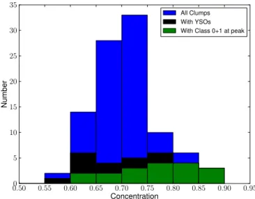
Figure5shows and Tables6and7record the distribution of submillimeter flux densities associated with the position of each YSO from the 850 μm maps. Most of the Class II and Class III YSOs are associated with little to no submillimeter emission at either 450 μm or 850 μm. This result is as expected (Dunham et al.2015)since those YSOs are more evolved, with small or non-existent surrounding envelopes and enough time has passed for them to have moved from their natal surroundings. The younger Class 0/I and Flat YSOs are seen to be embedded in regions of higher flux emission, appropriate for dense envelopes and/or proximity to material responsible for their birth. While there appear to be a subset of Class 0/I Table 7

(Continued)

YSO Indexa _R.A.b _Decl.b _{Class Type}c _F

850d F450d AVd Hoste Neareste Distance

(J2000.0) (J2000.0) (Jy/Bm) (Jy/Bm) mag Clump Clump (arcsec)

1817 21:53:32.0 +47:16:03 II −0.009 0.01 6.07 L 85 72.4 1819 21:53:33.0 +47:16:09 III 0.001 0.29 6.11 L 85 71.8 1821 21:53:33.2 +47:13:41 II 0.074 0.15 6.00 82 82 34.2 1822 21:53:33.4 +47:11:16 II −0.013 0.01 5.85 L 82 179.2 1824 21:53:34.0 +47:15:55 II −0.014 −0.16 6.11 L 85 54.6 1825 21:53:34.1 +47:16:04 III −0.022 −0.21 6.11 L 85 62.4 1827 21:53:35.7 +47:12:26 III 0.020 0.12 7.00 L 87 109.7 1828 21:53:35.8 +47:12:12 II 0.009 0.03 7.00 L 87 123.5 1829 21:53:36.2 +47:10:27 II −0.012 0.09 5.79 L 93 193.2 1832 21:53:38.2 +47:14:59 II 0.037 0.06 6.22 85 85 19.6 1834 21:53:38.4 +47:12:31 II 0.021 −0.11 7.47 L 87 105.6 1835 21:53:38.7 +47:12:05 II 0.004 0.02 7.32 L 93 124.0 1836 21:53:38.9 +47:13:27 II −0.004 0.17 7.49 L 87 53.1 1837 21:53:40.0 +47:15:26 II 0.039 −0.06 5.61 90 90 8.6 1838 21:53:40.4 +47:15:08 II 0.031 0.08 6.22 90 90 19.7 1839 21:53:40.6 +47:16:49 II −0.003 0.11 5.50 L 88 58.0 1840 21:53:40.8 +47:15:42 II 0.003 0.19 5.61 L 90 14.8 1842 21:53:42.1 +47:15:53 II −0.009 −0.15 5.08 L 90 28.8 1843 21:53:42.5 +47:18:25 II 0.039 0.05 5.56 L 92 59.5 1844 21:53:45.2 +47:12:35 II −0.000 0.24 5.81 93 93 54.5 1845 21:53:46.5 +47:14:35 II 0.021 0.05 6.38 L 91 39.9 1847 21:53:51.6 +47:16:48 II −0.002 −0.06 4.06 L 92 75.9 1848 21:53:51.8 +47:07:11 III −0.017 0.06 0.85 L 93 322.4 1850 21:53:57.9 +47:19:34 II −0.018 0.02 2.82 L 92 170.0 1852 21:54:00.3 +47:25:22 II 0.020 −0.14 1.09 L 81 354.7 1853 21:54:01.4 +47:14:21 II 0.016 −0.10 4.91 96 96 62.5 1854 21:54:06.0 +47:22:05 II 0.005 −0.19 1.37 L 89 319.6 1855 21:54:08.7 +47:13:57 II 0.000 0.25 3.39 L 96 130.9 1856 21:54:12.5 +47:14:35 II −0.023 −0.01 1.84 L 96 174.4 1857 21:54:18.7 +47:12:09 II 0.007 −0.07 1.43 L 95 255.2 Notes. a

YSO observation designation from Dunham et al. (2015).

b

Location of YSO.

c

YSO Class (see the text).

d

See text for definitions.

e