Constraining model biases in a global general circulation model with ensemble data assimilation methods

(1)

Constraining model biases in a

global general circulation model

with ensemble data assimilation

methods

Martin Canter

GHER, GeoHydrodynamics and Environment Research

Department of Astrophysics, Geophysics and Oceanography

University of Liege

A thesis submitted for the degree of

Docteur en Sciences

(2)

(3)

Committee members

Prof. Jean-Paul Donnay, President (University of Li`ege) Prof. Jean-Marie Beckers (University of Li`ege)

Prof. Hugues Goosse (SST/ELI/ELIC, Universit´e Catholique de Louvain) Directeur de recherche CNRS Pierre Brasseur (IGE, Universit´e Grenoble Alpes) Dr. Charles-Emmanuel Testut (Mercator-Ocean)

Dr. Fran¸cois Counillon (Nansen Environmental and Remote Sensing Center) Dr. Alexander Barth (University of Li`ege)

(4)

I would like to thank my thesis supervisor, Dr. Alexander Barth. He initially gave me the opportunity to discover and awaken my interest for numerical modelling and oceanography during my master thesis. During the four years of my PhD, his support, expertise and advices guided me through the multiple difficulties of this research. He was always available and never failed to provide a response to any of my question.

I would like to thank Prof. Jean-Marie Beckers the insightful review of my work, and the multiple ideas to be explored, especially during the very pleasant DIVA workshops.

I would like to thank the rest of my thesis committee, Prof. Jean-Paul Don-nay, Prof. Hugues Goosse (SST/ELI/ELIC, Catholic University of Louvain), Di-recteur de recherche CNRS Pierre Brasseur, Dr. Charles-Emmanuel Testut, and Dr. Fran¸cois Counillon for the careful review of this manuscript.

A special thank to Arthur Capet, who helped me through the first months of my PhD, and shared his office with me.

I would also like to thank my colleagues from the GHER, Sylvain Watelet, A¨ıda Alvera Azcarate, Thi Hong Ngu Huynh, Charles Troupin, Stephane Lesoinne, Igor Tomazic, Subekti Mujiasih, Gaelle Parard and Svetlana Karimova for the Friday afternoon coffees and the ensuing discussions and presentations who made me dis-cover other aspects of oceanography.

To my upstairs and downstairs neighbours and colleagues, Maxime Hubert, Se-bastien Mawet, and Christophe Becco, I want to express my thanks for your help, encouragements, and questions which provided me with a different point of view on my work.

I am also thankful to the two wonderful persons who organise all the events around the GHER, Charlotte Peelen and C´ecile Pregaldien.

A special thanks to Manon Mathieu, without whose support throughout those four years this thesis would not have been possible.

(5)

V

I would like to thank two friends, Romain Van der Keilen, and Werrick Deneu, whose companionship and help to solve programming issues have been immensely helpful.

A special thank to my family, whose encouragements helped me through all my levels of educations.

This work was funded by the project PREDANTAR (SD/CA/04A) from the federal Belgian Science policy (http://www.climate.be/PREDANTAR) and the San-goma FP7-SPACE-2011 project (grant 283580) (http://www.data-assimilation.net/).

Alexander Barth is an F.R.S. - FNRS Research Associate. Computational

re-sources have been provided by the Consortium des ´Equipements de Calcul Intensif

(C´ECI), funded by the Fonds de la Recherche Scientifique de Belgique

(F.R.S.-FNRS) under Grant No. 2.5020.11. MDT CNES-CLS09 was produced by CLS Space Oceanography Division and distributed by Aviso, with support from CNES (http://www.aviso.altimetry.fr/).

(6)

(7)

Abstract

A new method of bias correction using an ensemble transform Kalman filter as data assimilation scheme is developed. The objective is to cre-ate a stochastic forcing term which will partially remove the bias from numerical models. The forcing term is considered as a parameter to be estimated through state vector augmentation and the assimilation of ob-servations.

The theoretical formulation of this method is introduced in the gen-eral context of numerical modelling. A specially designed and modified Lorenz ’96 model is studied, and provides a testing environment for this new bias correction method. Several different aspects are considered through both single and iterative assimilation in a twin experiment.

The method is then implemented on the global general circulation model of the ocean NEMO-LIM2. The forcing term generation is detailed to respect particular physical constraints. Again, a twin experiment allows to assess the efficiency of the method on a realistic model. The assim-ilation of sea surface height observations is performed, with sea surface salinity and temperature as control variable. Subsequently, a multivari-ate assimilation shows further improvement of the bias correction.

Finally, the method is confronted to real sea surface height observations from the CNES-CLS09 global mean dynamic topography. A thorough study of the NEMO-LIM2 model response to the bias correction forcing term is proposed, and specific results are highlighted. An iterative as-similation concludes the method investigation. Possible ideas and future developments are suggested.

(8)

(9)

Abstract

Une nouvelle méthode de correction de biais utilisant un filtre d’ensemble de Kalman transformé est développée. L’objectif est de construire un terme de for¸cage stochastique afin de réduire le biais d’un modèle numérique. Ce terme de for¸cace est considéré comme un paramètre à estimer via l’augmentation du vecteur d’état lors de l’assimilation d’observations.

La formulation théorique de cette méthode est présentée dans le contexte de la modélisation numérique. Le modèle de Lorenz ’96, spécifiquement modifié dans le cadre de cette étude, permet de disposer d’un environ-nement controlé pour éprouver la méthode de correction du biais. Une expérience jumelle est utilisée pour expérimenter ses différents aspects au travers d’assimilation successivement simple et itérative.

Cette méthode est ensuite implémentée sur le modèle global et général

de circulation de l’ocean NEMO-LIM2. La g´en´eration du terme de

for¸cage est détaillée afin de respecter différentes contraintes physiques et numériques. Une expérience jumelle permet d’évaluer l’efficacité de la méthode sur un modèle réaliste. La hauteur de la surface de la mer est considérée comme donnée d’observation et assimilée, la température et la salinité de surface de la mer servant de variable de contrôle. Enfin, ces deux premières variables sont assimilées simultanéement, permettant la comparaison avec l’assimilation simple.

Pour terminer, la méthode est confrontée à un cas opérationnel, avec des données de topographie dynamique moyenne provenant de CNES-CLS09. Une étude approfondie du modèle NEMO-LIM2 lors de l’application de la méthode de correction du biais est présentée. L’assimilation itérative de ces mêmes données cloture les expériences menées autour de cette méthode. Différentes idées de développements futurs sont proposées.

(10)

(11)

4.1.4 Discussion . . . 59 4.2 Practical formulation . . . 60 4.3 Experiment set up . . . 61 5 Lorenz ’96 Model 63 5.1 Model description . . . 63 5.2 Model characteristics . . . 64 5.3 Model modification . . . 66 5.3.1 Model average . . . 67 5.3.2 Spatial average . . . 68 5.4 Single assimilation . . . 73

5.4.1 Bias correction results . . . 74

5.5 Iterative assimilation . . . 75

5.5.1 Observations batches creation . . . 78

5.5.2 Experiment set-up . . . 79 5.5.3 Results . . . 80 5.5.4 Conclusion . . . 84 6 NEMO-LIM2 87 6.1 Model presentation . . . 87 6.1.1 Primitive equations . . . 88 6.1.2 Boundary conditions . . . 89 6.1.3 Subscale processes . . . 90 6.1.4 ORCA2 grid . . . 91 6.1.5 Implementation . . . 92

6.2 Mixed layer depth . . . 93

6.3 Bias in NEMO-LIM2 . . . 94 6.3.1 CMIP5 . . . 94 6.3.2 Preparation work . . . 96 6.3.3 Seasonal Cycle . . . 96 6.3.4 Internal Variability . . . 98 6.3.5 Conclusion . . . 99

(13)

Contents XIII 6.4.1 Horizontal structure . . . 100 6.4.2 Stream function . . . 101 6.4.3 Vertical extension . . . 102 7 Twin experiment 111 7.1 Monovariate assimilation . . . 111 7.1.1 Model variability . . . 111 7.1.2 Error adjustment . . . 113

7.1.3 Forcing field correction . . . 114

7.1.4 Model rerun . . . 116 7.1.5 SST and SSS validation . . . 117 7.2 Multivariate assimilation . . . 119 7.3 Conclusion . . . 122 8 Realistic case 127 8.1 Single assimilation . . . 127 8.1.1 Global SSH . . . 128 8.1.2 Analysis confidence . . . 130 8.1.3 Final correction . . . 133 8.1.4 SST Validation . . . 134 8.2 Iterative analysis . . . 136 8.2.1 Experiment set-up . . . 136 8.2.2 Results . . . 137 8.2.3 SSH average error . . . 138 8.3 Conclusion . . . 139 9 Perspectives 143 9.1 Development options . . . 143 9.1.1 3D forcing . . . 144

9.1.2 Time dependent forcing . . . 145

9.2 Validation . . . 145

9.2.1 Method comparison and combination . . . 145

9.2.2 Parametrisation . . . 146

9.2.3 Localised corrections . . . 147

10 Conclusion 149 11 Appendix 153 11.1 Inverse of block matrix . . . 153

(14)

11.2 Equivalency of bias estimator . . . 156 11.3 Lorenz long term averages . . . 158 11.4 List of variables . . . 159

(15)

Chapter 1 Introduction

1.1 Historical perspective

Historically, in 1922, Richardson published the first attempt at a numerical forecast of weather (Richardson, 1922; Lynch, 2008). His so called ”forecast factory”

inter-polated available observations to build initial conditions at t0. From there, by hand,

he produced a 6-hour forecast of the atmosphere over two points in central Europe, using a hydrostatic variation of Bjerkness’ primitive equations. The results were, unfortunately, completely unrealistic, resulting in a surface pressure over a six-hour period of 145 hPa (Lynch, 2006). The simple interpolation used did not respect the physical constraints, therefore developing unstable modes which eventually con-ducted to model instability. Moreover, the initial conditions were unnatural. This inevitably led to spurious tendencies and imbalance between the pressure and wind fields. Despite the generally favorable reviews of his work, the impracticality of his method with the available tools deterred others to follow his path for a couple of decades.

It is only with the arrival of computers that weather prediction and climate mod-elling would again be conceivable. In the early 1950’s, a team was able to produce 24-hour forecasts, which needed 24 hours of computation. It was the first time that

(16)

numerical weather prediction was able to keep up with time. Improvements in nu-merical analysis, with new and stable algorithms, the development of data retrieval tools, such as satellites, and the introduction of data exchange, provided a solid and fertile ground for further research in numerical modelling of the earth.

The close relationship between the atmosphere and the ocean, whether it be the physical properties and transfers between both, or the similarities regarding the numerical particularities of those systems, led to ocean modelling to follow the path of weather prediction. Two major operational differences remain between the two geofluids. The first resides in the interest of producing daily forecasts of those systems: the need for daily atmospheric weather forecasts did not originally find a similar interest in ocean modelling. It is only recently that the need for seasonal and inter-annual oceanic forecasts arose. In particular, the influence of the ocean on global climate, and the prediction of large-scale phenomena linked to the ocean,

such as El-Ni˜no, required a knowledge of oceanic processes to be available

before-hand. There is also an interest in short-range forecasts (on an oceanic scale) for e.g. world navies, fisheries, off-shore drilling, search and rescue operations, or oil spill forecasts. The second difference relates to the available data sets, which are consid-erably smaller for the ocean. The ocean, compared to the atmosphere, is a harsh environment which strains data collection systems. Whereas, on the continents, ob-servations stations have been monitoring the weather for a long time, similar tools could not be used in the ocean. For a long time, due to the necessity of having a human performing the measurements, oceanic measures only relied on boats sailing through the ocean. It is only since the arrival of electronics that automatic drifters and buoys have provided regular data sets. The rise of satellites also greatly helped to provide large coverage for the size of the oceans. Consequently, the available measures of the ocean still lack sufficient coverage for extended time periods, and for remote regions.

Nonetheless, numerical modelling of geophysical systems brings a certain num-ber of problems which can not be ignored. Examples are the limitation that comes from the finite computational power available which results in limited resolution, imperfect specification of boundary conditions, and poor representation of sub-grid physical processes. The initialization of a model also requires either a climatology based on another model or retrieved through observations, or an excellent knowl-edge of the system, in order to avoid early imbalances in the model. All those issues require a particular treatment with specifically developed methods.

(17)

1.2. Data assimilation 3

1.2 Data assimilation

One of those methods is data assimilation. It is a technique developed to handle the difficulties that arise from numerical modelling. It describes a method which aims at determining the state of a model by combining heterogeneous and imperfect observations in an optimal way. In particular, its purpose is to correct numerical models representing an dynamical system for which observations are available. A perfect representation of a real dynamical system is not possible. As such, compro-mises have to be made, and lead to poor processes parametrisation and approximate initial states. Errors are therefore inevitable, and need to be coped with, in order to obtain a more accurate estimation of the state of the system.

Data assimilation can be summarised as the combination of mathematical algo-rithms which incorporates observations into the model state of a numerical model, using prior error and statistical information about both the observations and the model state, and the mathematical equations describing and governing the model. Those available information are all different in nature, quantity and quality. Com-monly, the state of the model prior to assimilation is called the forecast, and the result of the assimilation is then an optimal representation of the model state which is called the analysis.

A concrete example can easily be detailed for the weather forecast. After taking the temperature in two cities during a couple of days, one wishes to forecast the daily temperature in the forthcoming days, for both cities, and the land that separates them. A relatively straightforward method is to extrapolate the evolution of the temperature, assuming that the measurements curve is smooth enough. One could also rely on a statistical database of previous evolution of temperature. With the help of numerical modelling, one could also aim to forecast the temperature through simulations. On the next day, the forecast can be compared with the real weather. By taking new measurements in both cities, the model forecast can be corrected. However, supposing that no data is available for the space separating both cities, the model would still also need correction at those points. Finally, errors on the measurements need also be to taken into account. Data assimilation techniques try to optimise those corrections by using the available information about the model and the measured data.

(18)

Originally developed for meteorology and numerical weather prediction, data assimilation dates back to the 1950’s (Panofsky, 1949) , and has a long history of applications in many different fields such as oceanography, glaciology, seismology, nuclear fusion, medicine, agronomy, ... The recurring common factor of data as-similation applications is inaccurate numerical models for which observations are available. In particular in geoscience, with high dimensional systems, the number of observations and the huge number of variables in the system, respectively up to

107_-109 _{nowadays, are a real issue and impose constraints due to the limited}

com-putational power available.

At first, empirical methods were developed. The successive corrections method (SCM) dates back to 1955 (Bergthörsson and Döös, 1955), and is an iterative process which starts with a background field or first guess. A linear weighing scheme is then used to adjust the initial guess and subsequent estimates to fit the grid point values to the observations, taking into account the ratio of the observation error variance to the background error variance (Cressman, 1959). It was improved later by Barnes (1964) for analyses where no available background field could be provided. Bratseth (1986) showed that SCM can be made to converge to a optimal interpolation pro-vided that adequate weights are chosen.

Data assimilation methods can currently be divided into different categories, de-pending on their inherent hypotheses, and their approaches. In essence, they can be either sequential or nonsequential. In sequential assimilation, the model is in-tegrated over a period of time with no available observations. When the model reaches a point in time where observations are present, it is stopped. The model is then used as a first guess or background estimate which needs to be corrected or updated with the observations. The statistical information about the model and the observations error are used to obtain the best corrected state, or analysis. The model is then restarted from that point in time. This process is repeated until all observations are used. One can thus look at sequential data assimilation as a suc-cession of integrations and corrections over a period of time where observations are distributed and available. The particularity of sequential data assimilation is that the observations are only used to correct the model forward in time. There is no backwards correction of the previous or initial state from later observations.

(19)

relax-1.2. Data assimilation 5

ation. In this method, an additional source term, or sink term, is added to the prognostic equations of the observed variables. This will then nudge the solution towards the observation (interpolated to the model grid) during the integration of the model equations. Hence, nudging has a continuous effect on the model, at every time step. A relaxation time scale is chosen based on empirical considerations. A too short relaxation time and the solution will converge too fast, causing imbalanced model states. A too long relaxation time causes model errors to grow too large. Ex-ample of this method application are altimetry assimilation in the North Atlantic (Blayo et al., 1996), or a 15 year reanalysis from the ECMWF (European Centre for Medium-Range Weather Forecasts) (Kaas et al., 1999). In practice, nudging is easy to implement, and the computational cost is nearly negligible. However, it is not applicable when using indirect observations, and unobserved variables have to adjust themselves through the model dynamics. Still, nudging is still used for spe-cific applications, such as the assimilation of gridded data from a reanalysis. More recently, Auroux and Blum (2005) proposed a back and forth nudging, using an inverse source term and integrating the model backwards in time to the initial state. Optimal interpolation is also a sequential assimilation method (Gandin and Hardin, 1965). Unlike nudging, optimal interpolation uses physical assumptions and error statistics. For instance, one can connect sea surface temperature and altimetry to general circulation models, such as will be used later in this work. Op-timal interpolation refers to methods originating from linear estimation theory. It is based on a background error covariance matrix which is assumed constant in time. More recently, optimal interpolation schemes using a different parametrisation for the error covariance matrix and its numerical representation have been developed, such as the multivariate optimal interpolation scheme (Daley, 1991), or the ensem-ble optimal interpolation scheme (Oke et al., 2002), used in Counillon and Bertino (2009) to forecast the Loop Current in the Gulf of Mexico.

3D-Var is another sequential assimilation method (Courtier et al., 1998). The idea is to provide the model state as input, which is then adjusted in such a way that the model output is as close as possible to the observations and to the back-ground field. 3D-Var can be seen as a variational method in the sense that it requires the development of the adjoint of the observation operator. Therefore, the model dynamics is not involved, and the relationship between the model state and the observations is performed through the adjoint. If this observational model is linear, 3D-Var becomes equivalent to optimal interpolation.

(20)

The Kalman filter, and its numerous derivations, are also sequential methods (Kalman, 1960). Essentially the background and its error covariance matrix are computed and updated at each assimilation cycle. It assumes that the errors are additive, unbiased, uncorrelated and Gaussian distributed for the model and the observations, and that the model and observation operator are linear. The extended Kalman filter proposes to linearise the model dynamics and the nonlinear observa-tion operator (Jazwinski, 1970). The Kalman filter and the extended version can not be used directly on realistic models, where the model dynamics is nonlinear, causing the error covariance matrix to become difficult to compute. An interesting derivation of the Kalman filter is its ensemble formulation, known as the ensemble Kalman filter (Evensen, 1994). It was introduced to overcome the the limitations of the first-order approximation of the extended Kalman filter through a Monte Carlo approach. The full derivation of the Kalman filter, the extended Kalman filter and the ensemble Kalman filter, is detailed in chapter 3. Because of their efficiency, robustness, and the ease of implementation, the Kalman filter and all the existing modifications are very popular in geophysical applications (Edwards et al., 2015).

The particle filter eliminates the need for the Gaussian assumption required by the Kalman filter (DEL MORAL et al., 1995; Van Leeuwen, 2009). Therefore, it handles the nonlinearities much better than the Kalman filter. It is directly drawn from the Bayes theorem, without any additional assumption. Each ensemble mem-ber (similarly to the ensemble Kalman filter) is called a particle, and is integrated through the nonlinear model. The objective is to represent the posterior probability function without any prior assumption on its distribution. When observations be-come available, the information contained in the observations is incorporated into the particles. Probabilities based on an estimated likelihood function resample then the ensemble, and provide a new analysed ensemble. The particle filter is also a sequential assimilation method. It is however difficult to apply to realistic cases due to the curse of dimensionality of high dimensional data and state spaces, causing a large number of particles to be required.

In nonsequential assimilation methods, the information is propagated both for-ward and backfor-wards. This allows the estimation of a past model state based on posterior observations. For example, the Kalman smoother (Gelb, 1974) is an ex-tension of the Kalman filter which uses past and future observations by integrating the time dimension into the state vector. In Cosme et al. (2010), a square-root

(21)

1.2. Data assimilation 7

smoother algorithm is presented as an extension from the singular evolutive ex-tended Kalman filter (Pham et al., 1998). The same generalisation can be applied to the particle filter, which is then called a particle smoother (Tanizaki, 2001).

Another class of nonsequential assimilation methods are adjoint methods. They are powerful tools that provide and estimate of the sensitivity of a model output with respect to an input. In particular, in data assimilation, an optimal analysis is one that fits the observations best, using assumptions and available information about the error characteristics of the data used. This is where adjoint methods perform efficiently, allowing the optimization problem to be solved in a reasonable time for application to real-time forecasting (Errico, 1997). Basically, adjoint methods make use of adjoint of the model whose solution is being examined (hence, ”adjoint”), where the adjoint is formally defined as the transpose of the tangent linear model. A control solution and a measure of the forecast are considered. The gradient of this forecast at the control solution is evaluated with respect to perturbations of each component of the model output. This gradient can be interpreted as the sensitivity of the forecast to the perturbations. Those perturbations can be on the initial con-ditions, boundary concon-ditions, or even model parameters.

However, adjoints methods also show limitations. The model equations have to be differentiable, which is not always the case (Zupanski et al., 2008). One also needs to store either the complete trajectory, or to be able to partially recompute it to evaluate the adjoint. This involves sophisticated check-point techniques to efficiently solve the problem. The derivation of the adjoint (and the tangent lin-ear) model can prove to be difficult and tedious. Some improvements in automatic adjoint compilers have been performed, but the procedure is still challenging (He-imbach et al., 2005). Additionally, the cost-function might have a local minimum, causing the minimisation to converge only to the local minimum, and not the global one. In particular, for 4D-Var, if the probability density function has multiple sec-ondary modes, finding the global one can be a challenge.

4D-Var is a nonsequential data assimilation method which makes use of the ad-joint of the model (Dimet and Talagrand, 1986; Talagrand and Courtier, 1987). It is able to take all observations into account. However, all error sources must be control variables of the optimisation process. Since one can not take into account the error introduced at every time step, the model is assumed to be perfect. This

(22)

is imposed as a strong constraint. One can interpret the 4D-Var scheme as an time extension of the 3D-var. 4D-Var is still commonly applied to various practical cases in oceanography (Ngodock and Carrier, 2014; da Rocha Fragoso et al., 2016).

In the representer method (Bennett, 1992), the model error is accounted for, unlike the 4D-Var method. However, this can be prohibitive if a lot of information are available, such as satellite data coverage.

1.3 State of the art

Bias is commonly defined as a systematic error with a nonzero mean. In a more formal formulation, any kind of component of error which is systematic, with regard to the notion of the average of a model or estimator, can be considered as bias (Dee, 2005). The effects of bias can significantly deteriorate the model solution. Bias can take multiple different forms, spatially variable, seasonal, or even depend on specific situations. In numerical modelling, current limitation comes among others from the finite computational power available, which, in ocean models, results in limited resolution. With inaccurate surface forcings, those are examples of model associated bias. The limited knowledge of the system also leads to imperfect specifi-cation of boundary conditions, and poor representation of subgrid physical processes (Baek et al., 2009). Those differences between the numerical model and the dynam-ics of the real ocean induce systematic errors in the numerical forecasts. Daytime high-altitude radiosonde temperatures can be biased due to solar radiation effects, and radar altimetry affected by electromagnetic bias originating from the smaller reflectivity of wave crests than troughs, are examples of observation related bias (Ghavidel et al., 2016). Finally, bias can even come from the assimilation itself, when unbiased observations are assimilated into a biased model. The model drift towards its biased state causes bias in the assimilation, and can lead to apparent changes in characteristics of the observing system (Santer et al., 2004).

When used for prediction, or long term simulations with a limited number of available observations, those systematic errors cause the model to exhibit significant differences in climatologies when compared to the reality. In some circumstances, they can even be comparable or larger than random or nonsystematic error of the model solution. While the random part of the model error has been reduced thanks to several advances in numerical modelling, it has become increasingly necessary to address the systematic model error (Keppenne et al., 2005). The bias in climatic

(23)

1.3. State of the art 9

modelling can be so large, that only variation and anomalies are studied rather that the absolute model results (Zunz et al., 2013).

In the context of oceanography, state of the art ocean models exhibit significant differences in the climatological mean state when compared to observations from the real ocean (Flato et al., 2013). For instance, eddy-mean processes can be poorly represented, which causes western boundary currents to be responsible for large sea surface temperature bias, such as for the Gulf Stream and the Kuroshio currents (Large and Danabasoglu, 2006).

To reduce the error of the model, one can make use of data assimilation schemes. However, a critical assumption for analysis schemes is that the mean of the back-ground error is zero. This hypothesis is clearly violated in the presence of bias. Data assimilation schemes that are designed to use nonbiased observations to correct ran-dom errors with zero mean in a model background estimate, are called bias-blind. In presence of bias, those analysis schemes are suboptimal, and can generate spurious corrections and undesired trends in the analysis (Dee and Uppala, 2009). Most data assimilation schemes are designed to handle small, random errors and make small adjustments to the background fields that are consistent with the spatial structure of random errors (Dee, 2005). Unfortunately, due to the systematic character of model errors, their representation as random errors, or noise, is rather poor. In some cases, such as satellite observations, bias can even be larger that the actual, useful signal present in the observations (Cucurull et al., 2014).

Bias-aware data assimilation scheme are designed to simultaneously estimate the model state variables and parameters that are set to represent systematic errors in the system. However, assumptions need to be made about the error covariance of the bias and its attribution to a particular source. It also needs to be represented and expressed in a set of well-defined parameters.

Model bias estimation was first introduced by Friedland (1969), and more deeply described by Jazwinski (1970); Gelb (1974). He suggested a scheme in which the model state vector should be augmented with a decoupled bias component that can be isolated from the other state vector variables. This allows the estimation of the bias prior to the estimation of the model.

(24)

et al., 2005; Chepurin et al., 2005). In offline methods, bias is estimated from the model mean and the climatology, using a preliminary model run. Offline methods are simple to implement and have a small computational cost. In online methods, bias is updated during the data assimilation step, resulting in an analysed bias.

The most known and referred to algorithm for online estimation and correction of the bias in sequential data assimilation is presented in Dee and Da Silva (1998). Bias is estimated during the assimilation by adding an extra and separate assimilation step. It was successfully applied in Dee and Todling (2000) to the global assimila-tion of humidity observaassimila-tions in the Goddard Earth Observing System. A simplified version of this algorithm using a single assimilation step (where Dee and Da Silva (1998) needed two) was applied by Radakovich et al. (2001) to land-surface temper-ature assimilation, and by Bell et al. (2004) for the online estimation of subsurface temperature bias in tropical oceans. It was also used for model bias estimation by Baek et al. (2006), and observation bias correction in Fertig et al. (2009). In Carton et al. (2000b), a 46-year global retrospective analysis of the upper-ocean tempera-ture, salinity and currents, was performed, with bias originating both from model limitations and poor surface forcings. In Keppenne et al. (2005), bias between the climatology of the model and the data was problematic for the use of satellite al-timeter data from TOPEX/Poseidon. In Chepurin et al. (2005), the effect of bias on a 31-year long historical analysis of the physical state of the ocean is studied, with a focus on the mixed layer and thermocline depth in the tropical Pacific Ocean, and in Nerger and Gregg (2008), a singular evolutive interpolated Kalman filter was extended with an online bias correction scheme.

However, a critical requirement is that most methods of bias correction need a reference data set which is defined as bias free, from which a bias estimation can be provided. In practice, it can be difficult to find such a data set. The bias also needs to be charaterised in terms of some well-defined set of parameters. While this is obvious for bias estimation, it is a critical condition when attempting bias correction. The attribution of bias to an erroneous source will force the assimilation to be consistent with a biased source. In some cases, the bias correction would even deteriorate the assimilation procedure, and perform worse than a classic, bias-blind assimilation (Nakamura et al., 2013; Massari et al., 2015).

Hence, the effect of bias on the model climatology can not be neglected. The ne-cessity of removing, or at least, reducing the effects of bias on the model has driven

(25)

1.3. State of the art 11

to the development of methods allowing to force the model towards a nonbiased climatology. Addressing systematic model errors, such as oceanographic biases, is even more tricky, since a representation of the bias itself, or the generation mech-anism, is needed. The bias in the background field can be directly modelled by assuming some kind of persistence (Dee and Da Silva, 1998; Chepurin et al., 2005). Background errors (defined as the nonzero mean residuals) being observable, it is rel-atively straightforward to formulate a consistent bias-estimation scheme. Suppress-ing the bias generation durSuppress-ing the integration of the model would even be preferable.

For example, in Derber and Rosati (1989), a variational continuous assimilation technique is applied. In the same way as nudging for data assimilation, it is a modi-fication of the adjoint techniques, where a correction term is added to the equations, in order to correct the bias. It aimed at optimally fitting the data throughout the assimilation period, rather than relaxing the solution towards the values at observa-tion times. It has been applied to radiative transfer model in Derber and Wu (1998).

Another example is in Radakovich et al. (2004), the model is so heavily affected by bias that a classic bias aware assimilation scheme (Dee and Da Silva, 1998) is not sufficient enough. The bias correction term is only applied during the assimila-tion scheme, but due to the model characteristics, it quickly slips back to its biased state and dissipates the correction term. In that study, an adapted incremental bias correction term was applied, during the model run, proportional to the initial state and the time separating two analysis steps (Radakovich et al., 2004). In some cases, the bias is handled through a post integration bias correction (Stockdale, 1997).

Recently, Vossepoel et al. (2004) evaluated the possibility of reconstructing wind stress forcing fields with both a random and constant error part, with a 4D-Var assimilation scheme on a twin experiment. Leeuwenburgh (2008) performed the estimation of surface wind-stress through an ensemble Kalman filter and corrected the boundary conditions of the model, effectively reducing the model bias. A very similar study to the work presented here is Ngodock et al. (2016), where an extra term is introduced in the tidal forcing, to correct errors in the tide model due to imperfect topography and damping terms.

(26)

1.4 Objectives

In this work, the problematic of model bias correction is tackled by developing a new method which combines stochastic forcing and data assimilation. While most previously developed and existing methods correct bias in the model results, the objective here is to come closer to the origin of the bias, and correct it by applying a stochastic forcing into the model equations. Data assimilation, and in particular the Ensemble Transform Kalman Filter (ETKF) is used, in a similar way to parameter estimation, to tune and find an optimal forcing term which is directly injected into the modified model equation. The aim is to provide a continuous bias correction by forcing the model.

The initial motivation to develop a new bias correction method arose in the con-text of the PredAntar project (Goosse et al., 2015), which consisted in the study of the Antarctic sea-ice coverage during the period 1980-2009 through the use of the coupled sea ice ocean NEMO-LIM2 model. Considering the long integration period of the project, compromises were made to respect the multiple limitations inherent to the project, such as a coarse model resolution. These caused the model to suffer from bias. Reanalysis throughout the model run provided adequate corrections, but highlighted the effects of bias, and the current bias correction methods limitations. This novel approach is detailed in a general Kalman filter theoretical framework to prove its theoretical consistency. The successive steps are carefully detailed in the context of data assimilation, so that it can easily be transposed from the current oceanic application to any biased numerical model.

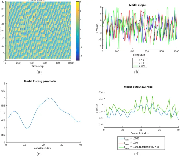
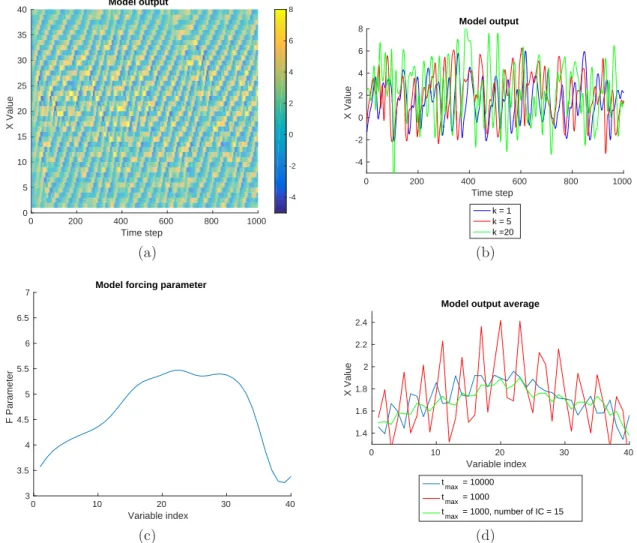
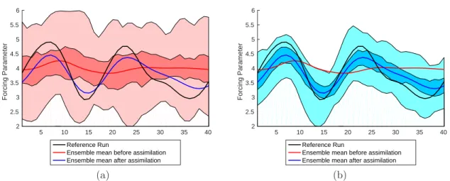
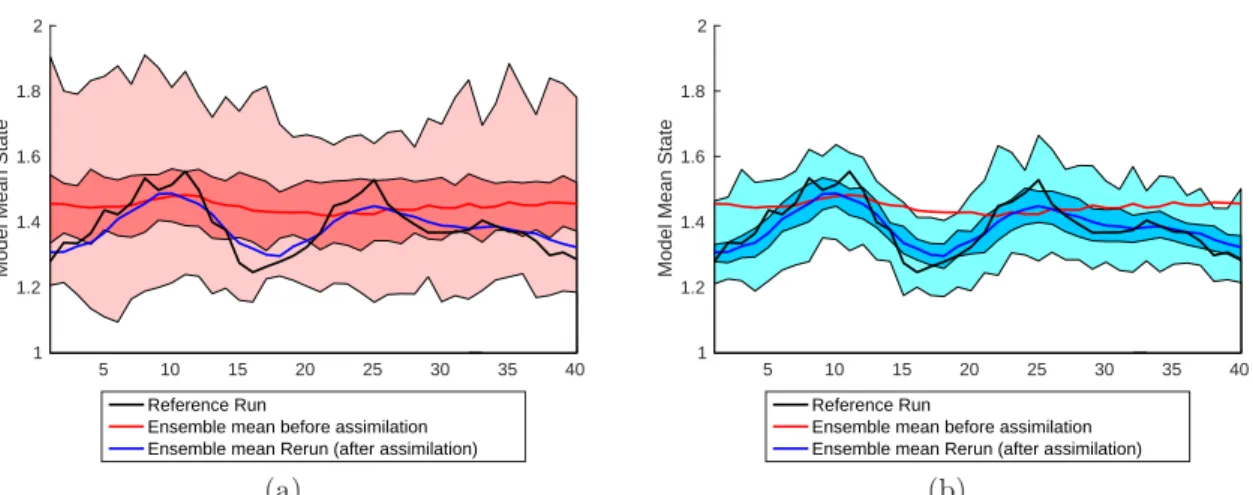
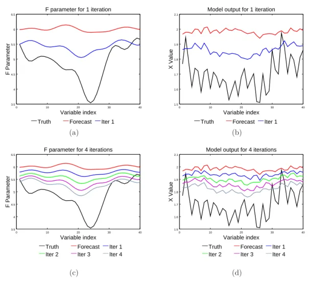
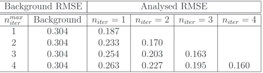
For the first application of the new bias correction method, the classic Lorenz ’96 mathematical model (Lorenz, 1996; Lorenz and Emanuel, 1998) is chosen for its chaotic characteristics. Necessary modifications are applied to adjust the model to the specific needs of this study. Hence, the modified Lorenz ’96 model characteristics are investigated to show particular connections to realistic ocean models. A classic twin experiment on a Lorenz ’96 model is then implemented to test the efficiency and adaptability of the new bias correction method. Results are presented and studied in the context of a single assimilation procedure. Since applying a forcing in a nonlinear model exposes one to a nonlinear response of the model, an iterative assimilation is performed and compared to the single assimilation experiment.

(27)

1.4. Objectives 13

The encouraging results of the Lorenz ’96 twin experiment lead to the applica-tion of the bias correcapplica-tion method to the coupled sea ice ocean NEMO-LIM2 model. This model is presented in the context of its recent use in a research project, with a comparison with similar models from the CMIP5 framework, and bias affecting the model results is highlighted. The new bias correction method is implemented to the NEMO-LIM2 model, respecting particular constraints. Again, a twin experiment is used to test the stability of the forcing term generation and the efficiency of the bias correction. A single and monovariate assimilation is performed, showing model response to the forcing. A second multivariate assimilation shows the improvement obtained when more observations are used to estimate the bias correction term.

Finally, the method is confronted to a realistic case using real observations from the CNES-CLS09 global mean dynamic topography. A single assimilation experi-ment shows the effect of the different choices of the bias correction ensemble gen-eration. The model response to the forcing term is interpreted in relation to the general circulation of the ocean. An iterative assimilation is also performed, and indicates the nonlinear model response to the forcing term.

(28)

(29)

Chapter 2 Basic concepts

In this chapter, the basic concepts required for the comprehension of the work presented in this thesis will be listed and detailed. Most of them are assumed to be known to the data assimilation community in numerical weather prediction and oceanography through general use and practice. With the intention to keep this work as clear as possible, the notation used will respect the unified notation for data assimilation (Ide et al., 1997) where relevant.

2.1 The model

In numerical modelling, the aim is to describe and reproduce a system through a set of discrete equations. This set of equations is called a numerical model. When applied to oceanography (or other geosciences for instance), models are partial, sim-plified and sometimes inadequate representations of the real world. It is clear that a model can never describe the whole complexity of the ocean. Choices, assumptions and hypotheses have to be made in order for the model to be viable in practice. De-pending on the objective of the model, constraints are applied on the resolution, the

(30)

number and type of processes represented, etc. For instance, biological processes are not necessary for a physical ocean model of the long term Antarctic sea ice coverage. Still, numerical modelling is an essential and powerful tool for scientific inquiry. Controlled experiments (Lyard et al., 2006), the influence of the variation of a parameter (Baker et al., 2013), or ”what if” scenarios (Dufresne et al., 2013), can help to understand which processes are important, and which assumptions are valid.

A numerical model forwards its model state in time using prognostic variables. Prognostic variables such as temperature, velocity or salinity, are necessary for the model calculations. They are regrouped into the state vector which uniquely de-scribes the state of the system at a particular point in time. The model forwards prognostic variables from the model state at the previous time step. They can be compared to diagnostic variables, which help to interpret the model state, but can always be reconstructed from prognostic variables. An example of prognostic variable is the horizontal velocity, which depends on the horizontal velocity of the previous time step. However, the vertical velocity does not require the previous time step, but can be directly derived from the model state at the required time, making it a diagnostic variable. One must be able to distinguish between a complex reality, which can not be truthfully represented by a set of numbers, and the best way to represent reality as a state vector of a numerical model.

Formally, based on the state vector xm−1 at a time tm−1, with the subscript

m = 1, ..., mmax being the time index, the model allows to compute the state vector

xm at the following time step tm. With M being the forward model operator, one

can write that

xm = M(xm−1). (2.1.1)

The successive model states defined by equation (2.1.1) can be referred to as the model trajectory. The model trajectory describes the path of the different model variables, hence the model state, during the time period over which the model is run. The trajectory can be written as follow (van Leeuwen, 2001; Hunt et al., 2004)

(31)

2.2. State vector augmentation 17 x′ =       x1 x2 ... xmmax      . (2.1.2)

2.2 State vector augmentation

A common procedure in numerical modelling is the state vector augmentation. In-deed, whereas the prognostic variables of the model are sufficient to fully describe the state of the model, it can be necessary to include other variables in the state vector, such as additional forcing (which will be extensively used in this thesis), scalar parameters, or diagnostic variables. In practice, one can algorithmically ex-tend the state vector by appending the additional variables to the state vector. One can rewrite equation (2.1.2) by augmenting the state vector with one or multiple variables e as x′ =         x1 x2 .. . xmmax e         . (2.2.1)

State vector augmentation is commonly used in parameter estimation (Barth et al., 2010; Sakov et al., 2010), for the parameter to be estimated needs to be present in the description of the model through the state vector. A key advantage, in particular for Kalman filters, is that the incremental cost of an augmented-state vector is relatively small compared to the cost of the state vector alone (Kondrashov et al., 2008).

2.3 Parameter estimation

In numerical modelling, one needs to configure the numerical model through a series of well-defined parameters. Those parameters can contain errors, and contribute to some part of the model error. Parameter estimation inherently considers that the

(32)

parameters should be treated as variables of the model. One can include parame-ters in the state vector through state vector augmentation (equation (2.2.1)). Those parameters can be either fixed, or have a spatial and/or temporal evolution. For example, Bryan (1987) carries out a series of experiments on a low resolution, prim-itive equation ocean general circulation model to study the processes controlling important aspects of the circulation, and in particular the sensitivity of the model to the magnitude of vertical diffusivity. In Bergman and Hendon (2015), monthly radiative fluxes and heating rates are determined from monthly observations of cloud properties from the International Satellite Cloud Climatology Project and temper-ature and humidity from ECMWF analysis.

It is common for parameters to be strictly positive or constrained, such as the albedo of the ocean. Parameters are often also difficult, if not impossible, to measure directly (Losa et al., 2004). Optimally estimated parameter can attain nonphysical values due to either overfitting of data, or lack of identifiability with the available data. The complex and often nonlinear feedback between parameters is a particu-lar issue if one wants to increase the number of parameters estimated at the same time, hence the dimension of the estimation problem (Navon, 1998). Parameters can also be updated locally, independently of their properties. In particular, if a global parameter is updated differently in a local assimilation scheme, one can use the different analysed values of said parameter to estimate the optimal global value. One of the earliest applications of direct parameter estimation in oceanogra-phy using contemporary techniques was the estimation of the Cressman term of a barotropic model used for the parametrisation of the divergence associated with long waves (Rinne and J¨arvinen, 1993). Good parameter tuning is crucial in numerical modelling. In Zhu and Navon (1999) for instance, a complex global spectral model with its adjoint were used to tune both parameters and initial conditions. They concluded that even though the initial conditions dominated in the early stages of assimilation, the optimality of model parameters had a greater importance and persisted much longer than optimal initial conditions. Different approaches for pa-rameter estimation have been tested and explored in the past literature.

For instance, adjoint methods borrowed from the optimal control theory can adjust model parameters through the use of available data. However, the model is supposed to be perfectly known and without error, which is never the case for practical applications in oceanography. One can choose to account for the errors of

(33)

2.3. Parameter estimation 19

the parameter estimation problem, but this greatly increases the dimension of the control space (Ten Brummelhuis et al., 1993). In some cases, extending the dynami-cal model equation (equation (2.1.1)) with the parameter to be estimated can cause the system to become nonlinear, even if the original system were linear (Kivman, 2003). Gong et al. (1998) is another example of adjoint method application, where a simple linear model was used as equivalent to a barotropic vorticity equation for the stream function on a latitude circle. It concluded that physical parameters to which the analysis is sensitive can be tuned along with one or two weighting parameters, and a smoothing parameter. Nevertheless, adjoint models are not always available, and demand considerable efforts to be developed.

Batch calibration techniques assume the time-invariance of the parameters and rely on statistical measures to minimise the long-term prediction error over some period of calibration and validation data (Kuczera, 1983; Vrugt et al., 2003). They require a set of historical data to be stored and processed, which can be a com-putational burden. Sequential data assimilation techniques have also been used for parameter estimation in oceanic systems. They present the advantage of overcoming this drawback and being able to explicitly take into account both the uncertainties on the model parameter, and the uncertainties of the model structure, its input, and its output (Moradkhani et al., 2005). The Kalman filter is a classic example of recursive data-processing algorithm, but it is limited to linear dynamic models with Gaussian error statistics. The extension to nonlinear systems with the EKF using first order linearisation can be used, but leads to instabilities when the nonlinearities are too strong (Miller et al., 1994).

Ensemble Kalman filters are also used for parameters estimation. In the EnKF framework, those parameters can be an unabridged part of the analysis and be up-dated along other model variables (Annan et al., 2005a). One of the first uses of the EnKF for parameter estimation occurs in Anderson (2001), where a demonstration is performed on a Lorenz ’96 model by developing an ensemble adjustment Kalman filter. As suggested by Derber and Rosati (1989), the state vector is augmented with the parameters to be estimated. The analysis then contains both the updated conventional state variables, and the newly estimated parameters. In Aksoy et al. (2006), the performance of an EnKF is investigated through a simultaneous state and parameter estimation, where the source of the model error is contained in the uncertainty of the model parameters. The large scale applicability of the EnKF has also been highlighted by Annan et al. (2005a) in an earth model of intermediate

(34)

complexity. In Kondrashov et al. (2008), a coupled ocean-atmosphere system is in-vestigated and shows that the simultaneous estimation of two erroneous parameters and the model state allows the improvement of the model state and of unobserved variables.

Kivman (2003) highlights a severe drawback of any Kalman filtering scheme: due to utilizing only first two statistical moments in the analysis step, it is unable to deal with probability density functions that are badly approximated by the normal distribution. In that study, an extension of the sequential importance resampling filter is proposed in order to deal with strongly non-Gaussian distributions. It also highlighted the benefits of specifically developed nonlinear methods like particle fil-ters for non-Gaussian framework. Particle filfil-ters can be seen as variance minimizing schemes for any probability function (Simon and Bertino, 2012), which allows them to much better handle nonlinear parameters estimation. However, one must be care-ful when using them for large scale systems, as the size of the ensemble required is too large for realistic applications.

For large scale applications, the EnKF remains a practical and high-performance choice for parameter estimation. It scales much better than variational methods to large models. Additionally, it does not require the use of a linear tangent and ad-joint model, making it straightforward to implement. Bertino et al. (2003) suggested an extended framework in which a nonlinear change of variables is applied in or-der to solve the obstacles posed by the non-Gaussian distribution of the variables. This procedure is called anamorphosis and allows the analysis step to be performed with transformed Gaussian distributed variables. Simon and Bertino (2009) demon-strated the feasibility of this technique in realistic configurations. In Simon and Bertino (2012), an improvement of the deterministic EnKF is proposed through such a Gaussian anamorphosis extension and solves in particular the inability of the EnKF to estimate negative parameters. This technique is also confirmed in Doron et al. (2013), where a combined state-parameter estimation in a twin experiment of a 3D ocean-coupled physical and biogeochemical model is successfully performed.

2.4 The observation operator

The model state at time m can be described by a vector xm. Each element of xm

(35)

compo-2.4. The observation operator 21

nents, coefficients, etc. One can also make use of observations ym, which represent

a specific measurement of a quantity at time m. The difference between the model

state xm and the observations ym resides in the fact that there is not necessarily a

one-to-one correspondence between the two quantities, and of course, only a small fraction of the state vector is observed (directly or indirectly). The observations are, in fact, rarely located exactly on the model grid points. Some interpolation might be necessary to obtain observation values on the model grid. Additionally, observa-tions are not always exact measurements of any variable of the model. An example is the sea surface temperature, where most recent SST global fields are not direct measurements of the ocean with a thermometer, but rather reconstructed satellite measurements of the ocean radiation.

To relate the observations with the model, one can determine a model equivalency of the observations through the observation operator H (Lorenc, 1986). Hence, one can express that

ym = Hm(xm) + ǫm, (2.4.1)

where ǫm is the observational error, whose covariance matrix is R, and which

consists of instrumental and representativeness errors with respective covariance

ma-trices Oi and Or. One thus has that R = Oi+ Or. The instrumental error is rather

straightforward, and represents the error coming from the instrument making the measurement of the observed quantity. On the other hand, the representativeness error is more complex. It represents unresolved processes by the model and is also called the unresolved scales error. It does not correspond to a problem with the observations, but is inherent to inadequacies in the dynamical model.

An example of the representativeness error for the sea surface temperature is the difference between the quantity measured by satellites, which is the skin tempera-ture, and the model surface temperature. Whereas the skin temperature represents the thin layer at the surface of the observed fluid, whose thickness is less than 500µ m, the actual model surface temperature is much thicker, of the order of the meter (5 m for the NEMO-LIM2 model, section 6.1). The representativeness error is gen-erally much larger than the instrumental error.

The observation operator can be nonlinear, and can contain an explicit time dependence in addition to the implicit dependence via the state vector (Ide et al.,

(36)

1997). It contains the approaches required to make the correspondence between an observed quantity and the model-equivalent variable, through interpolation, complex transformation of model variables, integration, etc. In equation (2.4.1), one can interpret the observation operator as a sequence of separated operators transforming

the control variable xm into the equivalent of each observation ym, at the location

of the observations.

2.5 The observations

Observations are at the core of data assimilation. In this work, three different vari-ables will be used as observations for the purpose of assimilation, interpretation of the model results, and validation. Those three variables are sea surface height (SSH), sea surface salinity (SSS) and sea surface temperature (SST). However, SSS will not be further detailed, as it is only used as control variable in a twin experi-ment, and not in the realistic scenario.

As presented with the observation operator, one must keep in mind that the use of observations is not straightforward. It is necessary to specify how those observa-tions are initially defined, measured, represented on a grid and used for a particular objective.

2.5.1 Sea surface height

To define a height or a distance, one must first set a reference from which one can measure said distance. The difficulty to measure the SSH lies in the difficulty to determine those references.

To approximate the global shape of the earth (or other planetary bodies), geodesy defines a mathematical surface called the ellipsoid of reference. The level surface which corresponds to the surface of the ocean, when at rest, is called the geoid. It is close to the ellipsoid of reference which corresponds to the surface of a fluid under idealised homogeneous and rotating hypotheses, in a solid-body rotation and with no internal flow of the fluid (Stewart, 2008). However, the geoid differs from the ellipsoid due to local variations of the gravitational field. Those differences range up to 100 m (Lemoine et al., 1998). For example, seamounts are typically three times more dense than water, and increase the local gravity which causes a plumb line at the surface of the ocean. On the other hand, trenches in the oceanic floor tend

(37)

2.5. The observations 23

to create a deficiency of mass, thus a downward bulge. Finally, one must keep into account that the ocean is never at rest. Heat content of the water, tides, Rossby and Kelvin waves, eddies and ocean currents also affect the sea surface height, with ranges of up to 1 m. The deviation of the sea level from the geoid is defined as the dynamic topography. Formally, one defines the height of the geoid to the ellipsoid of reference as N, the sea level above the reference ellipsoid as η, and the sea level

above the geoid as h. One has that: h = η_{− N (Rio and Hernandez, 2004).}

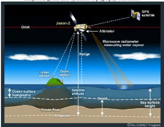
In practice, altimetry measurements are performed by radar on board of a satel-lite using high frequencies. The signal is reflected by the surface of the ocean. The time difference between the emission of the pulse and the reception of the echo allows the satellite to measure its distance to the sea surface. Even though the altitude of the satellite is determined by its orbit around the earth, which depends on the gravitational field of the earth, a precise knowledge of the geoid is not available. Hence, the SSH measurement provided by satellites are made with respect to the ellipsoid of reference. Parameters affecting those measurements, such as the speed of light in the atmosphere and interference from the ionosphere have to be taken into account. To provide a global coverage, the orbit of the satellite is chosen in order for the ground tracks to form a closed circuit after a predetermined number of cycles. Many altimetric satellites have flown in space to observe the ellipsoid of reference and measure the SSH. The most well-known space missions are Seasat (1978), geosat (1985–1988), ers–1 (1991–1996), ers–2 (1995–2011 ), Topex/Poseidon (1992–2006), Jason 1 (2002–2013), Envisat(2002), and Jason 2(2008-) (figure 2.1). In particular, Topex/Poseidon and Jason 1/2 were designed to provide a new level

of precision with an accuracy of_{±0.05 m. In a close future (2021), a joint mission of}

US NASA and French CNES (Centre national d’´etudes spatiales), called the Surface Water and Ocean Topography (SWOT), will be launched with a radar interferome-ter for making high-resolution measurements of the SSH. It will provide an increased spatial resolution to study ocean surface processes and circulation (Durand et al., 2010). Other ways to measure the SSH exist, in particular in situ measurements such as drifters or buoys velocities. The type of coverage required determines which measurement method is the most adapted.

Ocean models work with a grid which does not take the real geoid into account. Instead, they use a model geoid for which the sea level has a depth equal to zero when the ocean is at rest, in a constant gravitational field. The SSH of the model corresponds therefore to the dynamic topography. Hence, when one compares the

(38)

model SSH with the SSH obtained from altimetry measurements, one can actually only consider the anomalies to the zero level surface by subtracting the average SSH level from the data. In essence, the zero level surface is a measure of the total vol-ume of the ocean. This way, the difficulty of defining the exact geoid is removed.

Ellipsoid, geoid and dynamic topography schematic

Figure 2.1: Schematic of the Jason-2 mission, with the ellipsoid of reference, the geoid, the dynamic topography (here ocean surface topography) and the sea surface height. Adapted from https://www.eumetsat.int/jason/print.htm

The data set used in this work comes from the CNES-CLS09 global mean dy-namic topography (MDT) (Rio et al., 2011). It is a combination of GRACE data covering 4.5 years of measurements, altimetric measurements, and oceanographic

in situ _{data. It uses an optimal filtering method to compute the large-scale MDT}

first guess. The altimetric data was computed at the CLS (Collecte, localisation, satellite), for the 1993-2009 period. The in situ measurements comprise drifting buoys velocities covering the 1993-2008 period, for which an Ekman model allows the extraction of the geostrophic velocity component. Wind stress data needed to

(39)

2.5. The observations 25

estimate the Ekman currents come from the ERA INTERIM reanalysis covering the 1989-2009 period (Simmons et al., 2007). Hydrological profiles, in particular temperature and salinity, were measured by Argo floats from 2002 to 2008. The final product is a global mean dynamic topography of the ocean with a resolution

of 1/4◦ _{combining multiple different data sources, in particular satellites and in situ}

measurements.

2.5.2 Sea surface temperature

The importance of the ocean and its role in heat transport around the globe have been, in the last decades, the subject of major studies due to their relation to climate change (Wiens, 2016). The mechanisms with which exchanges take place between the atmosphere and the ocean are quite complex and include heat, momentum, moisture and gases. One can consider the SST as a global thermometer coupling the ocean and the atmosphere, which constrains the upper-ocean circulation and thermal structure. Similarly to the SSH, the most accurate SST products are pro-vided by the combination of multiple sources of satellite data, in situ data and the underlying processes.

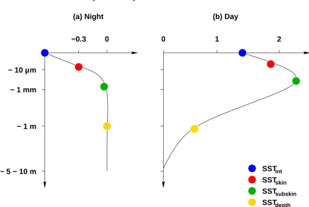
The water column extends from the surface to the ocean floor. Its vertical structure is both complex and variable. For global general circulation models and long term simulation, the vertical resolution is rather poor and the SST is considered as the temperature of the first layer of the ocean, with an order or magnitude of 10 m. One can easily realise the difficulty of measuring the SST by simply plunging one’s arm into the sea, detecting the surface temperature gradient of the water. In practice, one can classify the vertical structure of the SST from the surface to the depth as follow (Donlon, 2002):

1. SSTint, the interface SST between the atmosphere and the ocean. It represents

the infinitely thin layer where the ocean and the atmosphere are in contact, at

the top of the SSTskin layer. It can not be measured using current technology.

2. SSTskin, the skin SST is a thin layer of ∼ 500µ m of water, corresponding to

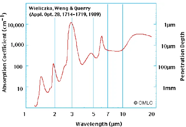
the maximum penetration of infrared waves. It contains the waterside air-sea interface where the conductive and diffusive heat transfer processes dominate. Depending on the magnitude of the heat flux, a strong temperature gradient can be maintained in this thin layer. Radiometers are typically used to measure

(40)

different penetration depths, the measured temperature varies depending on the measured wavelength (figure 2.2).

3. SSTsub, the subskin SST corresponds to the bottom on the SSTskin, at a depth

of_{∼ 1 mm. The molecular and viscous heat transfers dominate. It is measured}

by low-frequency microwave radiometers and has a typical timescale variation of minutes.

4. SSTbulk, the bulk SST or subsurface SST. This is the region beneath the SSTsub

where turbulent heat transfer processes dominate. It varies with depth, over timescale of hours and should also be noted with a reference to its depth:

SST5m. Buoys are used to perform in situ measurements of the SSTbulk.

The existence of the surface skin layer has been demonstrated both in theory (Hinzpeter, 1967) and practice (Schluessel et al., 1990). Its existence is required to regulate long wave radiation and turbulent heat fluxes across the sea surface. Indeed, turbulent eddy heat fluxes cannot transport heat across the ocean surface itself. The processes responsible for the heat transportation are molecular, hence the relatively thin size of the surface skin layer. Strong winds are able to destroy the skin layer through waves, but it is rapidly re-established when the waves dissipate.

The vertical temperature profile of the SST is shown on figure 2.3. One can easily note the difference between the day and night profiles, due to the presence or absence of the solar radiation.

2.6 Model skill

To assess the forecast skill of the model, one can compare the accuracy of the model trajectory and the degree of association to observations, expected or estimated val-ues of the model, persistence forecast (valval-ues of the predictand in the previous time period), or another model on which improvement is expected. This forecast skill, or just skill, is used both qualitatively and quantitatively. It can relate to localised or overall forecast performance according to metrics. It is commonly represented in terms of correlation, root mean square error (RMSE), mean absolute errors, Brier score, or bias, among others (Landman, 2015). For the skill study to be statistically robust, the skill score calculations should be made over a large enough sample. The study of the model output through its skill is in fact the primary target of numerical modelling. The model skill under all its forms allows the interpretation of the model

(41)

2.6. Model skill 27 Radiation optical penetration depth in water.

Figure 2.2: Radiation optical penetration depth in water. Adapted from Wieliczka et al. (1989).

results, and conclusions to be drawn.

Usually, forecast skill is presented as a percentage which is interpreted as a skill score and improvement over a reference, or a batch of observations. Formally, it is

characterised by a measure of accuracy A with respect to a reference Aref. With

Aperf being the value of the accuracy measure achieved by a perfect forecast, one

can represent the model skill as follow (Wilks, 2011)

SSref =

A_{− A}ref

Aperf− Aref · 100%.

(2.6.1)

If A = Aperf, the maximum value for the skill score SSref attains 100%. A = Aref

indicates no changes compared to the reference accuracy, with a skill score of 0%. A skill score between 0 and 100% implies an improvement over the reference, while

(42)

eas-Temperature profile of the sea surface

SST_int SST_skin SST_subskin SST_depth

(a) Night (b) Day

~ 5 − 10 m ~ 1 m ~ 1 mm ~ 10 µm

−0.3 0 0 1 2

Figure 2.3: Left hand side: Day profile. Right hand side: Night profile. Adapted from Donlon (2002).

ily be constructed by using the root mean square error as the underlying accuracy statistics, and one obtains

RMSE = v u u t 1 N N X i=1 (ˆx_{− x}i)2, (2.6.2)

where ˆx is the estimator of the estimated variable x from which the RMSE is

calculated.

In the next chapters, the skill score will not be explicitly used, but will be in some sense represented by the comparison of the RMSE values obtained from the different experiments.

(43)

Chapter 3 Theoretical framework

3.1 Kalman Filter . . . 29 3.1.1 Bayesian formulation . . . 30 3.1.2 Gaussian distribution . . . 32 3.1.3 Original Kalman Filter . . . 33 3.1.4 Best unbiased linear estimator . . . 37 3.2 Extended Kalman filter . . . 38 3.2.1 Nonlinear and non-Gaussian correction . . . 39 3.3 Ensemble Kalman filter . . . 42 3.3.1 The stochastic Ensemble Kalman filter . . . 44 3.3.2 Local assimilation . . . 48 3.3.3 The deterministic Ensemble Kalman filter . . . 49 3.3.4 The Ensemble Transform Kalman Filter . . . 51 3.4 Conclusion . . . 53

3.1 Kalman Filter

As presented in the introduction, numerical modelling and data assimilation re-late to a long history of developments and advances following practical needs and constraints. One popular method is the Kalman Filter (Kalman, 1960). Litera-ture related to Kalman Filtering is large, and dates back to its original expression, named after Rudolf Emil Kalman (who recently passed away, on the 2nd of July 2016). The first known application of the Kalman filter is to the nonlinear problem of space trajectory estimation for the Apollo program (Grewal and Andrews, 2010). The Kalman filter was incorporated to the Apollo navigation computer and used