Bottleneck resource allocation in manufacturing

HD28

.M414

Dewey

Bottleneck

Resource

Allocation in

Manufacturing

Anantaram

Balakrishnan

Richard

L.

Francis

Stephen

J.

Grotzinger

uiASSACHUSETTSUMSTiiure

OF

TECHNOLOGY

DEC

01

1994

Abstract

Many

resource-allocation problems in manufacturing and service operations require selecting integer-valued levels for various activities that

consume

"nondecreasing

amounts"

of limited resources.

System

productivity, to be maximized, is limited by the least productive (bottleneck) activity.

We

first review a basicbisection

method

that can solve thisdiscrete,

monotonic

resource-allocation

problem

even with nonlinear objective

and

constraints.

We

then generalize the basic algorithm to solve an

enhanced

version ofthe

problem

containing

additional coupling constraints on the allocation decisions. This generalization applies to assembly-release planning

(ARP)

in a multiproduct assemble-to-foreccist environment with part

commonality.

The

ARP

problem

requires finding feasible

amounts

of each product to release forassembly in each period using the available parts.

The

objective is to

maximize

the

minimum

difference

between

the actual and desired service levels over all products and time periods.

We

also consider extensions of the

ARP

model

incorporating precedence constraints

1.

Introduction

Many

resource-allocation

problems

in manufacturing

and

service operations require

choosing integer-valued levels for various activities that

compete

for limited,

common

resources in orderto

maximize

the

minimum

return or productivity over ail the activities. Applications of bottleneck

(max-min

or

min-max)

resource-allocation

models

include line

balancing,

raw

material allocation, maintenance planning, and storage allocation.

These

problems have the following general formulation. Let

X

be an n-vector of integer activity levels X:.

Each

activity

consumes

varying

amounts

of

m

resources. For i

=

1, ..., m, let

Sj and gj(X) denote, respectively, the total availability of resource i and the

amount

ofthis

resource

consumed

by

the activity levels in X. If fi(Xj) denotes the "productivity" ofactivity j,

the system's productivity f(X) is limited by the least productive or "bottleneck" activity, i.e.,

f(X)

= min

{fj(Xj):j

=

1, ..., n}.

We

must

select activity levels that

maximize

system

productivity while satisfying resource constraints,

and

lower and upper bounds,

B

=

(Bj) and

C

=

(Cj). This discrete, bottleneck resource-allocation

problem

hasthe following nonlinear,

integer

programming

formulation:

[P]

maximize

f(X)

=

f"'" f-(x:) (1)

j=l, ..., n J J

subject to

gi(X)

<

Sj

foralli=

1,...,

m.

(2)

B

<

X

<

C.and

(3a)

Xj integer for allj

=

1, ..., n. (3b)

We

assume

that as the activity levels increase the

amount

ofeach resource

consumed

does

not decrease, i.e., fori

=

1, ...,

m,

the resource-usage function gj(X) satisfies the following

monotonicity (nondecreasing) property: given any

two

integral vectors X' and

X"

satisfying the upper and lower

bounds

(3a), gi(X')

<

gi(X") if X'

<

X".

Most

practical resource-allocation

applications satisfy this assumption.

Nondecreasing

functions are quite general; they can

model

economies

ofscale in the resource constraints, including fixed charges (e.g., fixed cost,

setup time,

and

so on).

The

productivity functions f:(Xj)

need

not be monotonic.

We

only require fj(Xj) to be real-valued

and

defined for all integer activity levels in the closed interval [Bj, Cj].

We

assume

that the

problem

is feasible, i.e.,

X

=

B

satisfies constraints (2).

Past research on bottleneck resource allocation (see, for instance, Luss [1992] and Ibaraki and

Katoh

(1988) for reviews of this literature) has addressed continuous-variable versions of

the

problem

and/or

models

with special structure (e.g., a single resource or linear functions). For the discrete allocation

problem

with one linear resource constraint (i.e., a knapsack constraint), Jacobsen (1971) proposed a marginal allocation approach. Porteus and

Yormark

[1972] developed an

improved

bisection search algorithm to solve this special case, and

Brown

[1979] described efficient solution procedures for knapsack-sharing

problems

with piecewise linear

and

nonlinear productivity functions.

For problems with multiple resources.

Tang

[1988] developed an

0(m

n^) algorithm fora

linear

model

in

which

the resource-usage functions gj(X) are all linear (with nonnegative

variable coefficients), and the productivity fj(x:) of each activity is astrictly increasing linear

function.

The

method

finds an optimal integer solution

by

solving a sequence ofrelaxed

problems

without integer restrictions.

Tang

described various manufacturing applications of this model, including a storage space-allocation

problem

(also called the reel-allocation model,

see

Ahmadi,

Grotzinger and

Johnson

[1988]). All ofthese applications satisfy the

monotonicity (nondecreasing) assumption. Recently, Francis

and

Horak

[1993] described a bisection search

method

to solve the storage space-allocation problem.

The

method

is robust

and

easy to implement, and although its computational complexity is data-dependent, the

method was

quicker than Tang's algorithm in computational tests.

This paper, motivated

by

some

resource-allocation decisions in electronics manufacturing and assembly, explores extensions ofthe bisection approach to address these decision

problems.

One

ofthese applications is a

cleanroom

sampling

problem

described

and

formulated by Grotzinger and

Cooper

[1992] as a bottleneck resource-allocation

model

with a nonlinear objective function and a

monotonic

resource constraint. In this application, the activity levels are the sample sizes for n samples atn specified locations ofa cleanroom.

These

samples are required for an inspection plan to certify the cleanroom.

The

cost ofsampling varies by location,

and

increases withthe

number

of samples.

The

cleanroom

has a fixed

budget for sampling.

To

meet

the federal standard for certification as a particular class cleanroom, the

sample

average contaminant concentration at each location

must

be less than a prespecified class limit. Since the variance ofthe

sample

average at

any

location varies

inversely with the size ofthe sampleat that location, alarger sample size will increasethe

probability thatthe sample average at that location will be less than the class limit.

However,

the limited sampling budget introduces tradeoffs in allocating samples to various locations as

we

attempt to increase the overall likelihood that the

cleanroom

will be certified, i.e., the

likelihood that the sample average will be

below

the class limit at

aU

locations.

To

develop an

effective inspection plan, Grotzinger and

Cooper

proposed a bottleneck

model

to select sample sizes that minimize the

maximum

variance ofthe sample averages overall the locations subject

to a linear financial resource (budget) constraint.

They

developed a

method

to optimally solve

the continuous relaxation ofthis

problem

(i.e., permitting fractional sample sizes), and proposed heuristic adjustments to the fractional solution to obtain an integer solution.

In Section 2

we

review the basic bisection algorithm to solve discrete,

monotonic

(nonlinear) resource-allocation problems such as the

cleanroom

sampling

model

even with nonlinear (but nondecreasing) sampling cost functions that reflect

economies

of scale. In

Section 3,

we

describe a multiperiod assembly-release planning

(ARP)

problem

with

serviceability constraints introduced by Grotzinger and

O'Connor

[1993] for an assemble-to-forecast environment with part commonality. This

problem

can be formulated as a

monotonic

resource-allocation

model

with additional coupling constraints

on

the allocation decisions.

We

discuss

how

to adapt the bisection approach to solve this model. In Sections

4

and 5

we

consider

more

general

ARP

models

with precedence constraints

and

parts substitutability. In

Section4,

we

first motivate

ARP

models

with general precedence constraints governing the

allocation of resources; these precedence constraints might

stem

from

the interaction of

production planning decisions across products

and

time periods.

We

then describe

how

to

modify

the bisection approach to solve this

new

class of problems. In Section 5,

we

consider assembly-release decisions

when

part substitutions are permitted, i.e., if

we

run out of a

particular part,

we

can still produce products that normally use this part

by

using an alternate part

from

a specified set ofsubstitutes.

We

further extend the bisection algorithm to

incorporate substitutability of parts.

To

our

knowledge,

multiperiod

ARP

problems with

precedence constraints

and

substitutable parts are unstudied.

Our

concluding discussion in Section

6

includes a broad interpretation ofthe various extensions tothe

monotonic

resource-allocation

problem

[P] that this paper has addressed.

2.

Bisection

Method

for

Discrete, Bottlenecit

Resource

Allocation

The

bisection

method

for discrete, bottleneck resource allocation, although originally proposed for problems with linear productivity functions

and

resource constraints, also applies

to the nonlinear,

monotonic

version [P] ofthe problem.

However,

before applying the method,

we

must

replace any productivity functions that are not nondecreasing with equivalent

nondecreasing functions. In this section,

we

first describe the transformation,

and

then present

the bisection algorithm.

-3-Suppose

a given productivity function fX^\) is

nonmonotonic

or decreasing.

We

transform

it into an "equivalent" nondecreasing function fj(Xj) by setting

fj(Xj)

=

max

(fj(y): y

=

Bj, Bj+1 x} forall x

=

Bj. Bj+I Cj. (4)

This transformation, proposed by

Brown

[1991] for bottleneck problems with linear

knapsack

constraints, is also valid for problems with nonlinear, nondecreasing resource-usage functions.

To

confirm its validity, first note that fj() and f-() have the

same

maximum

values, and the

smallest value ofXj that

maximizes

fj(x:) is also the smallest value

maximizing

fjCx:), and vice

versa.

Using

this property,

we

can

show

that, ifthe resource-usage functions gj(X) are

nondecreasing, then the optimal objective function value ofthe transformed

problem

[P], with

fj() instead of fj(), equals the optimal value ofthe original problem. Moreover, the smallest

optimal solution

X*

to the transformed

problem

is also optimal for the original problem.

(Since the objective has the

max-min

form and

the resource-usage functions are

nondecreasing,

problem

[P] has an optimal solution

X*

that is

component-wise

less than or equal to all other alternate optimal solutions.)

Our

bisection

method

finds this smallest optimal solution. For convenience,

we

will

assume

in all ofour subsequent discussions that the

productivity functions are nondecreasing (i.e., the transformation (4) has been applied, if necessary).

We

refer to any vector

X

satisfying constraints (2) and (3) as a feasible solution.

We

seek an optimalfeasible solution

(OFS)

X*,

i.e., a feasible solution that

maximizes

f(X). Let z*

=

f(X*). Since the productivity functions are nondecreasing, f(B)

<

f(X)

<

z*

<

f(C) for any feasible solution X.

Given

any value z

e

[f(B), f(C)], define yj(z) by

yj(z)

=

rain {xj: z

<

fj(Xj). Xj

=

Bj,Bj+1 Cj} forall j

=

I. .... n. (5)

Thus, yj(z) is the smallest valueofthej'" activity level X: needed toensure that the productivity ofthis activity equals orexceeds z.

When

the inverse ofthe function fj() exists (for instance, if

fj() is linear), then

yj(z)

=

rfj"'(z)1 forall fj(Bj)

<

z

<

fj(Cj),

where

ful is the smallest integer

no

less than u. Otherwise,

we

can

compute

yj(z) using bisection search over the

domain

offj().

Given

any positive

number

e,

we

call afeasible solution

X

an

e-OFS

if its objective value is within e ofthe

maximum

value, i.e., if z*

-

e

<

f(X)

<

z*. Forthe linear model, Francis and

equivalent: (i) Y(z)

=

(y:(z)) is a feasible solution; (ii) Y(z) satisfies constraints (2);

and

(iii) z

<

z*. This result is the basis for their bisection algorithm. Both the result

and

the algorithm extend directly to discrete resource-allocation

problems

with nonlinear, nondecreasing resource-usage and productivity functions.

The

underlying idea ofthe algorithm is to iteratively select a trial objective function value z

at the midpoint of the current search interval,

and

check if the

problem

has a feasible solution

X

with f(X)

>

z.

We

check feasibility by first determining the smallest possible value yj(z) ofXj

needed

to ensure that the overall objective function value f(X) equals orexceeds z.

We

then

verify if the solution Y(z)

=

(yj(z)) satisfies the resource constraints (2). If it does, then Y(z) is a feasible solution to the problem, and sothe trial value z is a lower

bound

on the optimal value z* (actually, f(Y(z))

>

z is abetter valid lower bound);otherwise, z overestimates z*.

We

initialize the algorithm with lower and upper bounds,

LB

=

f(B) and

UB

=

f(C), on z*.

We

iteratively select z

= (LB

+

UB)/2, determine Y(z), and update

LB

to f(Y(z)) or

UB

toz depending

on

whether or not Y(z) satisfies (2). Iterations repeat until

UB

-

LB

<

e.

At

termination, the vector

Y(LB)

is an

e-OFS.

One

potential disadvantage ofthis approach is that its effort is data-dependent.

The

algorithm requires

up

to log2((f(C)

-

f(B))/e) iterations, each requiring n evaluations of the yj(z) values.

We

view

this disadvantage as principally theoretical in nature; typically, the datais not so big as to

make

bisection impractical.

The

polynomial-order algorithms proposed in the

literature

assume

special structure (e.g., linearresource constraints),

whereas

the bisection

approach is quite general.

3.

The

Assembly-Release

Planning

Problem

In this section,

we

review a production planning

problem

in an assemble-to-forecast

environment

with part commonality. Grotzinger

and

O'Connor

[1993] described

and modeled

this

problem

as a continuous, bottleneck resource-allocation problem. In this paper,

we

first

consider the integer version ofthis model.

The

problem

is formulated using variables for

cumulative production quantities instead of

monthly

(or weekly) production quantities.

The

resource constraints,

when

expressed in terms ofthese cumulative production variables, satisfy the nondecreasing property.

The

model

contains additional coupling constraints to ensure that the solution corresponds toa feasible production plan.

We

extend the basic bisection

the assembly-release planning

model

to account for precedence constraints and parts substitutability.

Assemble-to-forecast

(ATF)

or make-to-stock refers to systems that produce

goods

based

on

demand

forecasts rather than actual orders (see, for instance.

Baker

[1993]) because the procurement and production (fabrication or assembly)

Lad

times are longer than the customer

lead time (i.e., the time

between

placing an order and shipping the product to the customer). Electronics assembly facilities producing personal computers provide one

example

of an

ATF

environment. In this context, the procurement and assembly lead times could range

from

several

months

(to procure certain specialized integrated circuits) to a

few

weeks

whereas

customer

lead times might be only a

few

days.

The

personal

computer

assembly

example

also

illustrates another feature, part commonality, found in

many

ATF

environments.

Commonality

refers to using the

same

part (or

component)

for several different products. For instance,

several personal

computer models

might require the

same

microprocessor. Increasing part

commonality

provides

many

benefits including decreasing ordering

and

inventory administration expenses, and reducing safety stocks ofparts

due

to risk pooling (see, for instance, Bagchi and Gutierrez [1992], Baker,

Magazine

and Nuttle [1986], Collier [1982],

Gerchak

and

Henig

[1989], Gerchak, Magazine,

and

Gamble

[1988],

and

Grotzingeret al. [1993]).

In

ATF

facilities that produce multiple products with part commonality, decisions regarding

how

many

parts to procure in each period,

how

to allocate these parts to different

products, and

how many

"kits"

(component

sets for each product) to release for assembly in

each period

must

be based

on

estimates of probable future

demands

for each product, service

level requirements,

and

inventory considerations.

To

address these decisions, Grotzingerand

O'Connor

[1993]

developed

a general nonlinear optimization model,

and

formulated a linear

program

for a "feasibility

subproblem"

incorporating the parts allocation

and

assembly-release decisions.

We

focus

on

the integer version ofthis feasibility problem,

which

we

referto

as the assembly-release planning

(ARP)

problem.

We

next describe this problem.

Considera facility that assembles to forecast n (finished) products using

m

part types (or

parts).

Suppose

the procurement lead time is (p-t-l) time periods for all parts, and the assembly

lead time is

L

periods for all products. For simplicity, the

same

procurement lead time for all parts,

and

the

same

assembly lead time for all products, is assumed. Item-dependent lead times

are easy to incorporate.

The

parts ordered during the past p+1 periods will arrive at the beginning ofthe current period (t

=

0) and subsequently for periods, t

=

1, ..., p.

We

are

concerned with

how

to allocate these parts (including those currently on-hand) to various products,

and

how

many

kits to release for assembly during each ofthe _{next p} periods. Figure

1

shows

a timeline depicting various events: procurementdecisions, part arrivals, release of parts for assembly,

and

assembly completion.

We

assume

that the probability distribution of

demand

for every product during each of

the next (L+p) periods is given.

These

distributions are revised each period based

upon

current

market conditions and trends,

and

so the assembly-release plans

must

be updated each period. Since the assembly lead time is

L

time units, the

number

ofkits foreach product released for assembly at time t, for t

=

p,

must

be chosen to service the probable

demand

for that product in period (L+t).

The

planner's objective is to satisfy the

demand

foreach product in

every period L, ...,

L+p

with a given probability or target service level. Ifthe available inventory of a finished product in any period is less than the

demand

during that period,

we

assume

that the unsatisfied

demand

is backlogged.

We

define the cumulative availability ofa product attime t

>

as its initial inventory at

time t

=

plus the total output (i.e., completed assemblies)

from

period to period t.

The

actual service level fora product attime t is the probability that the cumulative availability of

that product attime t equals orexceeds its cumulative

demand

up

to

and

including time t.

The

target service level is the desired

minimum

value for this probability; this target might vary with

product and time period.

We

refer to the difference

between

the actual

and

target service levels as the service-level difference. Grotzinger

and O'Connor

[1993]

developed

a linear

program

to determine ifthe target service level can be achieved for all products

and

time periods using the

available parts,

and

if not to determine the

minimum

possible deviation

from

target.

The

model maximizes

the

minimum

service-level difference over all products

and

periods.

The

integer versionofthis model, the Assembly-Release Planning

(ARP)

problem, has the following

formal definition.

Given

the current parts inventory, the quantities

on

order

and

to be received during the next p periods, the bill of materials for each product,

and

the

demand

distributions for the next (L+p) periods, the

ARP

probl-^m seeks integer assembly-release quantities to

maximize

the

minimum

service-leveldifference overallproducts

and

timeperiods subject to parts availability.

Ifthe optimal objective function value is nonnegative, then the currently available parts

the desired service levels forall products in periods

L

through (L+p); the

ARP

solution

specifies a set of assembly-release quantities that meets the targets. Otherwise (ifthe optimal value is negative), the target service level cannot be attained for one or

more

products. In this

case, the assembly-release quantities specified by the

ARP

solution ensure that the actual service level is as close to target as possible. Grotzinger and

O'Connor

[1993] discuss

how

to decide

future parts

procurement

quantities based on the

ARP

solution.

Problem

formulation:

Forj

=

1 n, and t

=

0, .... p,

we

define nonnegative, integer variablesq:. representing the

number

ofunits of productj to be released for assembly in period t. For every part i

=

1, ...,

m,

let Hjj denote the

number

ofunits ofpart i used per unit ofproductj. For t

=

p, let S^^

denote the

(known)

cumulative supply ofpart i at time t, i.e.. Sj^ isthe

sum

ofthe initial

on-hand

inventory of part i at time plus the total anticipated receipts ofthis part during periods

through t.

Let Aj

j_^_| denote the

(known)

cumulative availability of (finished) productj in period

(L-I),

which

is equal to productj's current inventory (at time t

=

0, including assembliesjust completed) plus the total quantity released for assembly during the past (L-1) periods (i.e.,

from

period

(-L+1)

to period -I inclusive). For t

=

0, ..., p, the total

amount

of productj that

we

decide to release in periods through t (and will complete in periods

L

through (L+t)) is

qjQ+ ...

+

_q:j.

Adding

A:

j^j to this

amount

gives the cumulative availability ofproductj in

period (L+t). Let D: _j^^j be the cumulative

demand

(a

random

variable) for product j

from

period toperiod (L+t).

We

define

fjtCqio"'" •

•''^it)

^

*^^ service level difference for productj attime (L+t), i.e., for allj

=

1 n, andt

=

0, ..., _p,

fjj(qjO+ ... _-Kljt)

=

Prob{ Aj

l_,

+

qjQ

+

...

+

_qjj

>

Dj

l^,}

—

Target service level for productj in period (L+t).

The

minimum

service-level difference f(Q) is:

f(Q)

=

min{fj,(qjQ+

...+qjt):j

=

1 n,

and

t

=

p}. (6)

Note

that each f:,(),

and

hence f(Q), is a nondecreasing function ofthe release quantities, i.e.,

Q

<

Q' implies f(Q)

<

f(Q'). Also, fora given vector Q, every service-level difference function

fjj(q:Q+ ... _+qj() is nonnegative if and only iff(Q)

>

0.

[ARP]

maximize

f(Q) subject to:

n

Z

ajj _(q:Q

+

...

+

q-,)

<

Sj, forall i

=

1, ..., m, and t

=

p, (7)

j=l •* ^

q^

>

and integer for allj

=

1 n, and t

=

0, .... p. (8)

Constraints (7) ensure that the total

amount

of each part i used in all products during periods

through t does notexceed its cumulative supply Sjj.

We

wish to find nonnegative, integer

release quantities _qj^ to

maximize

the

minimum

service-level difference over all products and

all periods.

Although

formulation

[ARP]

has linear parts-availability constraints (7), our bisection solution

method

(described in the next section) also applies to problems with nonlinear resource constraints ofthe

form

G(Q) <

S,

assuming

that the vector function G(-) is

tier-nondecreasing

(TND),

i.e., if Q'

=

(qL) and

Q" =

(qj'j) are any

two

feasible solutions that satisfy

^]0

+

1j1

+

•••^jt

-

IjO "^^Iji

+

•••

+

'Ijt fo""allj

=

I n,

and

t

=

_p.

then G(Q')

must

be less than orequal to G(Q").

Note

that the objective function f() defined by (6)is also

TND,

but this property is not necessary.

We

can replace any given

non-TND

productivity function with an equivalent

TND

function, obtained by applying a transformation

analogous to equation (4).

Formulation

[ARP]

uses the service level differences as the productivity functions.

However,

the

enhanced

bisection

method

that

we

describe in the next section applies to the broader class of

problems

in

which

each productivity function f:j() is any real-valued and

well-defined function (not necessarily

TND)

of the cumulative availability of productj at time t.

As

a special case, considerthe

ARP

problem

with

known,

deterministic

demands.

Suppose, for each productj,

we

assign a penalty n- perunit shortfall ofcumulativeavailability relative to

cumulative

demand;

minimizing the

maximum

penalty over all products

and

time periods is

the objective function.

The

bisection

method

can solve this problem,

and

can also

accommodate

additional

TND

resource constraints, such as labor and budget constraints with

economies

ofscale and/orfixed charges. In Section 4,

we

consider further

model

extensions.

Solving

the

ARP

problem:

Let

Q

denote the set ofall feasible solutions

Q

satisfying constraints (7) and (8), and let z*

=

max[f(Q):

_Q

g

Q}.

Set

Q

is

non-empty

(since

Q

=

is afeasible

ARP

solution) and finite.

and so z* exists.

The

bisection

method

requires an initial search interval for the optimal value; therefore,

we

first develop upper

and

lower

bounds

on z*. Since the function f() is monotonic,

LB

=

f(0) is a valid lower

bound on

z*.

To

obtain an upper bound, note that for every

Q

e

Q,

ajj

(qjo

+

...

+

qj,)

<

S^

forall i,j, and t.

Thus, if

we

define

Ujj

=

min{LSjj/ajJ: i such that aj:

>

0}, (9)

where

LhJ isthe largest integer less than or equal to h, then, _qjQ

+

...

+

q-^

<

\i^ for all products

j

and

time periods t. Let

U

=

(Uj,). Since each function

(J)

is nondecreasing,

UB

=

f(U)

= min

{fjj(Ujj):j

=

1, ..., n and t

=

0, ..., _p} is a valid upper

bound on

z*. Furthermore,

_q^

<

yx-^ forall

J

and

t.

To

better understand

how

to adapt the original bisection approach tothe

ARP

model,

we

reformulate the

problem

by transforming the variables. Let

Xjt

=

_qjo

+

-

+

qjt forallj

=

1, ....n,

andt =

0, 1, ..., p, (10)

denote the cumulative release quantity of productj in periods through t. Replacing the

q-variables in formulation

[ARP]

with the x-variables,

and

defining

r(X) =

min{fjj(Xj,): j

=

1 n,

and

t

=

0, ..., _p}

we

get the following equivalent model:

[ARP']

maximize

f'(X)

subject to:

n

Z

ajj Xjj

<

Sjj for all i

=

1

m,

and t

=

p, (11)

j=l

'^jt

-

''j,t-l forallj

=

1

Xjj

<

Ujj for all j

=

1

x-j

>

and integer forallj

=

I

...,n,

and

t

=

1, ...,p, (12)

...,n,

and

t

=

0,1, ...,p,

and

(13)

..., n,

andt

=

0,1,...,p. (14)

The

coupling constraints (12), specifying that the cumulative quantity of productj released for

assembly at time t

must

equal or exceed its cumulative release quantity at time (t-1), reflect the

nonnegativity constraints

on

the variables

q^

in formulation [ARP].

Our

solution

method

does

not require the resource constraints (11) to be linear; it can also handle nonlinear resource

constraints

G"(X)

< S

as long as the function

G"(X)

is nondecreasing for all vectors

X

that satisfy constraints (12), (13)

and

(14) (requiring

G"()

to be nondecreasing is equivalent to our

previous

TND

condition

on

the resource-usage function G(Q)). Luss and Smith [1988] have considered a multiperiod

model

similar to [ARP'] but with continuous variables, linearresource

constraints, and hnear productivity functions fjt(Xj,) that represent the relative deviation of cumulative production

from

cumulative

demand.

Observation

1:

Every feasible solution

X

to [ARP'] has acorresponding feasible solution

Q

to

[ARP]

(with

the

same

objective value) and vice versa.

Proof:

Given

a feasible solution

Q

to

[ARP],

the solution

X

obtained using equation (10) is

feasible in [ARP'] and has the

same

objective value. Conversely, if

X

satisfies the constraints of [ARP'], then

we

obtain a feasible solution

Q

=

(q-j) to

[ARP]

with the

same

objective function value by setting

_q^

=

\^ -

x- _{j_j} forall t

=

1 p,

and

q:Q

=

Xjq for allj

=

1, .... n.

The

coupling constraints (12) differentiate

model

[ARP']

from

the basic

monotonic

resource-allocation

model

[P].

Note

that the function hjj(X)

=

X: _{j_|}

-

Xj^ is not

monotonic

in

X, i.e., X'

<

X

does not necessarily imply that hjj(X')

<

hjj(X). Therefore,

we

cannot include constraints (12) in the set of general resource constraints

G"(X) <

S, but need to treat

them

separately. Let us

now

explain intuitively

how

to

modify

the bisection

method

described in

Section 2 to handle these additional constraints. Recall that, for agiven trial value z ofthe

objective function value, the value yj(z) defined using equation (5) is the smallest value ofthe

resource-allocation variable x-

which

ensures that the objective value equals orexceeds z.

However,

these values might not satisfy the coupling constraints (12) in formulation [ARP].

Therefore,

we

modify

the definition ofthe y-values as follows. Forallj

=

1,2, .... n, and t

=

0,

1 p,let

Wjj(z)

=

min

{xjj: z

<

fjt(Xjj), Xjj

=

0. I, .... ^i^^}. (15)

We

then successively

compute

yu(z), fort

=

1, ..., p, as:

yjo(z)

=

Wjq(z), and (16a)

yjj(z)

=

max{yjj_,(z).

Wjj(z)}

ift>l.

(16b)

Note

that each _yi((z) is a nondecreasing function ofz.

Let il' denote the setofall vectors

X

satisfying (12), (13), and (14).

Observation

2:

For agiven value z

e

[LB, UB], the vector Y(z) obtained usingequations (16a) and (16b) is

the smallestelement ofQ' with an objective value ofat least z, i.e., Y(z) e ii', f'(Y(z))

>

z,

and

Y(z)

<

Y' forany other vectorY' e Q' with f"(Y)

>

z.

This observation stems

from

the monotonicity property of each function fjj(), and can be

proven using a contradiction argument.

Note

that, instead of using equation (16b),

we

can

equivalently define _yjt(z) fort

=

1 p, as

yj,(z)

=

min

(Xj,: z

<

fj,(Xj,), Xjj

=

yj ,_,(z), yjj_,(z)+l, .... Ujj}. (16c)

Observation 2

and

the monotonicity of the resource-usage functions

G"(X)

defined

by

(11) enable us to perform binary search to find an e-optimal solution to

problem

[ARP'].

We

first state this algorithm before justifying its validity.

The

algorithm contains an

embedded

search

procedure to evaluate Wjj(z) (defined in equation (15)).

We

refer to this procedure as the

W-evaluation subroutine.

Bisection

algorithm

for

ARP

problem

:

Step

0:

Initialization

P <— 0; {initial vector of lower

bounds

on Y(z*)}

Y<—

U; (initial vector of upper

bounds on

Y(z*)}

LB

<r- f'(0); (initial lower

bound on

z*}

UB

<r-

r(U);

(initial upper

bound on

z*}

Step

1:

Search process

REPEAT

z <-

(LB

+

UB)/2;

Compute W(z)

in _[P,Y]; (call W-evaluation subroutine}

FORj

=

l, ...,n. Set yjQ(z) <- Wjq(z);

FORt=l,....

p. Set yj((z) <-

max

|yj,_i(z), wjj(z)}; IF Y(z) satisfies constraints (11)

THEN

set

LB

<- r(Y(z))

and

p <- Y(z); (z

<

z*

and

Y(z)

<

Y(z*))

ELSE

set

UB

<- z

_{and Y}

<- Y(z); (z

>

z*

and

Y(z*)

<

Y(z)}

Step

2:

e-optimal

solution

FORj=l

n. Set qjo

=

yjo(LB);

FORt=

1,..., p, Setqj,

= yj,(LB)-yj,_,(LB);

Q

=

_(qj() ise-optimal.

W-evaluation

subroutine

:

To

compute

wjj(z) in _{[^^, y^] for} allj

and

t.

FORj

=

1 n,

FOR

t

=

0, ..., p.

Initialize

X

<r- _pj^ and \)<r- _Yjp

{pj,

<

Wjj(z)

<

Yjt} IF z

<

fj,(X)

THEN

setv<r-X;

ELSE

REPEAT

Set u <-L(A.

+

a))/2j; IF z

<

fjt(u)

THEN

set\><-u;

{Wj,(z)<u}

ELSE

set A. <— u+1; (u

<

Wj,(z) implies u+1

<

Wjj(z)}

UNTIL

X>\);

SetWjj(z) <— X);

Starting with

LB

=

r(0) and

UB

=

f'CU), the algorithm

computes

yjjCz), with z

=

(LB+UB)/2,

forallj and t; let Y(z)

=

(yj((z)). Ifthese values satisfy the resource capacity

constraints(1

1),

we

update

LB

<— r'(Y(z)); otherwise,

we

set

UB

<— z.

We

alsoupdate the upper

and

lower

bounds

on

the optimal values of

\^

(thus narrowing the search interval for Wjj(z)).

We

repeat this procedure until

(UB

-

LB)

<

e.

At

termination, the solution

Y(LB)

is e-optimal

for

problem

[ARP'].

We

recover the e-optimal solution to the original

problem

[ARP] by

setting the release quantity in each period t equal to the difference

between

the cumulative release quantities (given by the solution

Y(LB))

in periods t

and

(t-1).

To

compute

yj,(z),

we

first determine the smallest value Wjj(z) ofthe cumulative release

quantity for product_j at time t to achieve the objective function value z,

and

then apply

equations (16a) and (16b).

The

W-evaluation subroutine

employs

binary search in the interval

[PjpYjJ to determine Wjj(z). This subroutine is not necessary if

we

can directly evaluate the

inverse ofthe functions

fJ).

The

parameters _Pj^ and y-^ respectively denote the current lower

and upper

bounds

on the optimal value of the cumulative release quantity Xjj. _{Initially, Pj,}

=

and _Yj,

=

U:,. If the solution Y(z) at a particular iteration satisfies the resource constraints (11),

then Y(z) is a feasible solution to [ARP'j. Therefore, z*

>

z, and since the productivity

functions fjj() are nondecreasing, the

problem must

have an optimal solution

X*

satisfying

X*

>

Y(z). Hence,

we

increase the lower

bound

(3 to Y(z). Otherwise (ifY(z) does not satisfy

(1 D),

X*

<

Y(z) and

we

reduce the upper

bound

yto Y(z). Notice that, with this initialization

and updating scheme, the lower

and

upper

bounds

satisfy the following condition at every iteration:

Pj,t-1 - Pjt ^"'^ Yj,

^

Yj.,-1 forall j

=

1. ...., n, and t

=

1, ..., p.

We

emphasize that, since the release quantities

must

be integral, the W-evaluation subroutine

finds the exact value ofWjj(z).

The

validity ofthe bisection

method

rests

upon

the following result:

Proposition

3:

For the

ARP

problem

with nondecreasing resource-usage functions, a trial objective function value z is a lower

bound on

the optimal value z* ifand only ifY(z), defined by

equations (16a) and (16b), satisfiesthe resource constraints, i.e., iffG"(Y(z))

<

S.

Proof:

Let

X*

be any optimal solution to [ARP'] with optimal value z*

=

f'(X*).

The

solution

X*

is nonnegative, integral, and satisfies the resource capacity constraints (II) as well as the coupling constraints (12) and upper

bounds

(13).

Suppose

the trial value z is less than or equal to z*.

By

observation 2, Y(z) is the smallest nonnegative, integral vector

X

satisfying

constraints (12), (13), and f'(X)

>

z; therefore, Y(z)

<

X*. Since the resource-usage function

G"()

is nondecreasing and

X*

satisfies the resource constraints, Y(z)

<

X*

implies that G"(Y(z))

<

G"(X*)

<

S, i.e., the solution Y(z) satisfies the resourceconstraints. Conversely, suppose for a given valueof z, Y(z) satisfies the resource constraints (11).

By

definition, Y(z) also satisfies constraints (12), (13), and (14). Since z

<

r(Y(z))

and

Y(z) is a feasible solution to

[ARF],

z*

>

f

'(Y(z))

>

z.

Computational

effort:

To

find an e-optimal solution, the bisection algorithm requires at

most

log2((r(U)-F'(0))/e)

"major" iterations (i.e.,

number

of repeats in Step I). Since each service level difference is the

difference of

two

probabilities,

-2

<

fXO)

-

r(U) <

2. Therefore, ife

= 2"^^

=

1/1,048,576, no

more

than 21 iterations are required.

As

problem

size increases, the

method

will likely be

At each iteration, the

method

calls the W-evaluation subroutine n(p+l) times.

Each

evaluation requires at

most

_{log2(Yjt~Pit) iterations} within the subroutine.

We

can reduce the

search effort in the W-evaluation subroutine by modifying the overall algorithm as follows. At each iteration in Step 1, insteadof first evaluating

aU

the w-j(z) values before

computing

the

yjj(z) values,

we

firstevaluate Wjq(z),

and

set_yjo(z)

=

Wjq(z). Subsequently, fort

=

1 p in

sequence,

we

specify the lower

bound

ofthe search interval for the W-evaluation subroutine as

max{yj

_{t_i(z). Pjt)-}

Observe

that the values returned by the W-evaluation subroutine

now

directly correspond to the yj((z) values (i.e., they are not the Wjj(z) values

defmed

in equation

(15)). Since the search intervals are shorter, this modified

method

has lower computational

effort. Notice that, unlike

some

linear

programming-based

methods, the bisection

method

does

not introduce cumulative floating point errors. Finally, if

we

are not interested in the exact value of z* but only

want

to

know

ifz*

>

(i.e., whether

we

Ccin achieve the target service

levels forall products in all periods), then

we

can terminate the procedure as soon as

LB

becomes

nonnegative.

The

next

two

sectionsconsider

two

types of generalizations ofthe

ARP

model, namely, precedence constraints

and

part substitutability, that the bisection

method

can solve.

4.

Model

Extensions

I:

Precedence-constrained resource

allocation

The

ARP

problem

is a constrained version ofthe basic resource-allocation

model

[P], containing the additional coupling constraints (12) to ensure that the cumulative release in a period equals or exceeds the cumulative release in the previous period. Let us

now

consider a

broader class of "precedence" constraints that generalize the coupling constraints.

Our

initial

development

leads to our next generalization, (20) below,

which

is applicable to multistage

production settings.

Suppose

the production context requires that the cumulative release quantity ofa product_j at time t

must

equal or

exceed

the cumulative release quantity of productj' attime t', i.e.,

we

must

add constraints ofthe following type to formulation [ARP'] for a prespecified subset IP of

ordered product-time indexpairs <(j',t'),(j,t)>:

xjj

>

_Xj-f forall <a',t'). (j.t)>

e

IP. (17)

If<(j',t'),(j,t)> 6 IP,

we

say that (j'.t) 's apredecessorof(j,t).

We

will refer to discrete resource-allocation problems with precedence constraints (17) instead ofthe coupling constraints (12) as precedence-constrainedresource-allocation problems.

Let us define a precedence graph

PG

to encode the required relationships specified in the

set IP. This graph has one

node

for each product-time index (j,t), and contains a directed edge

from node

(j',t') to

node

(j,t) for every pair <(j'.t'). (j,t)> g IP.

Suppose

PG

contains a directed

circuit

DC.

To

satisfy all the precedence constraints (17) implied by the circuit

we

must

necessarily set all the variables corresponding to the circuit's nodes to the

same

value. Thus, if

N(DC)

denotes the set of nodes in the circuit

DC,

we

can reduce the size ofthe

problem

by

replacing X:jforevery (j,t)

e

N(DC)

by a single variable, say,

_\^q

in the resource constraints

(11); in the objective function,

we

eliminate fjt(Xjj) forall (j,t)

e

N(DC)

and instead introduce

^DC^'^DC^

= min

{fjt(X[)c): all (j,t)

e

N(DC)}.

Note

that this substitution preserves the monotonicity of the resource-usage and productivity functions. In the precedence graph, the substitution corresponds to contracting all the nodes (j,t) in the circuit into a single

node

DC;

all arcs originally incident

from

nodes not in

N(DC)

to any

node

in

N(DC)

are incident to node

DC

in the transformed graph.

By

successively eliminating all circuits in this manner,

we

obtain a circuit-free precedence graph

PG.

We

do

not require this graph to be connected.

Since

PG

contains

no

directed circuits,

we

can sequence its nodes such that foreach

node

(j.t) all its predecessors occur before it in the sequence. (This

node

sequencing operation,

analogous tothe

node

indexing

scheme

for

PERT/CPM

networks, requires

O(IEr)

computations,

where

lEl is the

number

ofedges in

PG;

see

Lawler

[1976].)

We

will refer to such a sequence

S

as a y-evaluation sequence.

We

can easily

modify

the bisection

method

to

accommodate

these precedence constraints as follows: in Step 1, after

computing

W(z)

in [p.y]

for allj

=

1, ..., n,

and

t

=

p,

we

considerthe indices (j,t) inthe y-evaluation sequence S, and set:

yj((z)

=

max

[wjj(z),

max

_{yj.t.(z): all (j'.f) such that<(j',t'),0,t)>

e

IP)]. (18)

The

remaining steps ofthe algorithm are unaltered. Again, the validity ofthis

method

stems

from

the nondecreasing property ofthe resource-usage

and

productivity functions.

For our original

ARP

problem

(described in Section 3), the set IP consists of index pairs <(j,t-l), (j,t)> for allj

=

1, .... n, and t

=

1, ..., p.

Observe

that the precedence graph

PG

for this special case of precedence-constrained resource allocation consists of n "line" subgraphs, one corresponding to each product; the adjacent nodes

on

each linej correspond to release

quantities forproductj in consecutive time periods. This precedence graph is circuit-free, and does not require any further reduction.

The

natural sequence ((j,t) forj

=

1, ...,n, t

=

0, ..., p)

satisfies the required precedence property; the original and

enhanced

bisection

methods

are identical if

we

use this sequence as the y-evaluation sequence S.

Let us

now

consider

how

to adapt the bisection

method

for discrete resource-allocation

problems with precedence constraints that are

more

general than constraints (17).

Suppose

product j is an accessory board

and

productj' _{is the}

_mother

_{board for a personal computer.}

The

production policy might specify that the cumulative release of productj at time t

must

equal or exceed a certain (nonnegative) proportion bjj:.j. ofthe cumulative release of product

j' _{at time} t' (t and t' might differ if the

two

board types have differentassembly lead times).

The

parameter h-^•^> might be based

upon

the relative yields of the

two

board types, spare parts

requirements, and so on.

Modeling

this policy requires adding precedence constraints ofthe form:

Xjj

>

_bjt

j.f Xj.j. forall <(j,t), (j'.t')>

6

IP. (19)

A

more

general version ofthese forcing constraints arises in multi-stage assembly settings

where

productj is a subassembly that is used in final assemblies_{jj, J2,} ....,_j^- Ifthe assembly

lead time for subassemblyj is k time units, b::. denotes the

number

of units ofproductj needed

perunit offinal assemblyj', and

Lq

represents the initial inventory of productj, then

we

require:

"jt "^ ^jO

-

_''jji ''ji.t+k

+

+

_''jjr

'^jr.t+k-This constraint specifies that the cumulative release ofsubassemblyj attime t plus the opening

inventory

must

equal orexceed the cumulative requirements ofthis subassembly to

meet

the

final assembly release quantities. In general, the precedence constraints might contain a (nonnegative) weighted combination ofseveral variables of the form:

where

the parameter e-^ is unrestricted in sign, but the coefficients

b^

:.j. are all nonnegative.

The

variable x-^ might be governed by several such precedence constraints, each with different

right-hand sides. Let n(j,t) denote the subset of precedence constraints (20) that contain the

variable Xj^ in the left-hand side, and let P:, be the set ofall indices (j'.f) such that Xj.^. occurs

with positive coefficient b-^•^• in the right-hand side ofat least one constraint of n(j,t).

We

refer to (j',t') as apredecessor of(j,t).

The

precedence graph

PG

for this

enhanced problem

has

one

node

corresponding toeach product-time index (j,t);

node

(j,t) has incident arcs <(j'.t'),0.t)> forevery (j',t') e P^^.

To

apply the bisection

method

for resource-allocation problems with the general

precedence constraints (19) or (20),

we

will

assume

that the corresponding precedence graph

PG

contains no directed cycles. (With constraints (19) or (20),

we

cannot always

make

the precedence graph acyclic using the successive substitution procedure

we

described for

constraints (17).)

The

multi-stage assembly

example

that

we

described earlier satisfies this

assumption. Since

PG

is

assumed

to be acyclic,

we

can sequence the product-time indices such that the index (j,t) occurs afterthe indices ofall its predecessors.

We

then determine the values y:j(z) in this sequence

S

using a generalized version of equation (18). This version

computes

y:,(z) as the

maximum

of w-j(z)

and

the highest right-hand side value over all the precedence

constraints in n(j,t).

By

considering the variables in the correct sequence,

we

ensure that the

values ofy:','(z) for all (j',t')

e

P^

are available before

we

compute

the value ofyjt(z).

We

can

extend the

same argument

to handle even non-linear precedence constraints x^

>

hjj(Yjj),

where

Y:j

=

{y:Y(z): all (j',t')

e

Pj^} as long as the functions h

_U)

are non-decreasing and the corresponding precedence graph is acyclic.

5.

Model

Extensions

II:

Part

substltutablllty

In Section 4,

we

showed

how

the bisection

method

extends toproblems with general

precedence constraints.

We

now

discuss modifications to incorporate another complicating feature of

some

electronics assembly environments, namely, part substitutability.

By

parts substitutability

we

mean

using adesignated alternative part (or parts) if the preferred part for a

product is not available.

Allowing

substitution yields risk-pooling benefits, and contributes to achieving desired service levels; however, it

may

also increase product costs

and

reduce product

quality and reliability. Products with substitute parts, although functional,

may

not be tested as thoroughly as the nominal design. Thus, it is desirableto allow

no more

substitution than is

needed

to achieve service levels.

Our

approach incorporates this preference, i.e., it exploits the

risk-pooling benefit of substitutability while maintaining cost, quality and reliability objectives. For

any

desired (and achievable) service level,

we

minimize the total

amount

(or cost) of substitution necessary by solving a

minimum

cost

network

flow problem.

Suppose

we

can replace part i with

some

other part without affecting the functionality of

the products. Let R(i) be the index setofparts that can replace part i,

and

let RB(i) be the set ofparts that can be replaced by part i, i.e., RB(i)

=

(i": i

€

R(i")}.

We

assume

one-for-one

substitution, i.e., one unit ofa part i'

e

R(i) replaces one unit ofpart i. Part substitutability, like

assemble products that require this part by using an alternate part

from

R(i). Klein, Luss, and

Rothblum

[1993] developed an efficient specialized

aigonthm

to solve linear, continuous

resource-allocation

problems

with substitutions.

Let us first formulate the assembly-release planning

problem

with part substitutability,

which

we

abbreviate as the

APS

problem.

As

before, let x-^ denote the cumulative release

quantity ofproductj in periods through t, forj

=

1, ..., n, and t

=

0, ..., p. For every part i, let bjQ be the initial availability ofpart i (i.e., opening inventory ofpart i in period plus the

quantity received in period 0), and fort

=

1, ..., p, let bjj be the

number

of units ofpart i

received in period t. In terms ofour previous notation, bjQ

=

Sjq, and h^^

=

Sjj

-

Sj j_[ fort

=

t

1, ..., p,

where

Sj^ is the cumulative availability ofpart i in period t.

Note

that Sjj

=

Z

bjj. for t'=0

all i and t.

As

before, \x^

=

min{LSjj/ajjJ: i such that aj:

>

0} is a valid upper

bound on

x-^.

For simplicity,

we

will consider the simple precedence constraints (12) specifying that x-j

must

equal or exceed x-_{j_|} forevery productj and periods t

=

1 p.

The model and

the modified

version ofthe bisection

method

that

we

describe later can also incorporate the

more

general

precedence constraints (19) or (20).

To

model

part substitutability,

we

introduce

new

"substitution" variables Vjji|, for all i

=

1,

..., m, i'

e

RB(i), andt

=

0, ..., p, denotingthe

number

ofunitsofpart i

used

toreplacepart i'

during

period t.

The

APS

problem

then has the following nonlinear, integer

programming

formulation.

[APS]

maximize

r(X) =

min{fjf(Xjf):j

=

1 n, and t

=

0, ..., _p} (21)

subject to:

n t t t

I

a- X-j

+

I

I

Vij. ,

<

I

bj,,

+

1

I

Vj,.; ,

j=l 'J J' t=Oi'eRB(i) t'=0 f=Oi"€R(i)

forall i

=

I, ...,

m, and

t

=

0,1, ...,p. (22)

Xjj

>

Xj

j_j forallj

=

1, ...,n,

and

t

=

1 _p, (23)

Xjj

<

Ujj forallj

=

1, ...,n,

and

t

=

0,1 p, (24)

Xjj

>

and integer for allj

=

1 n, and t

=

0,1, ...,p,

and

(25)

Vjj.j

>

and

integer

foraU

i

=

1, .... m, i'

g

RB(i). t

=

0,1, ...,p. (26)

19-Formulation

[APS]

is similar to our previous formulation [ARP'I except that constraints (22)

now

incorporate parts substitutability. and constraints (26)

impose

nonnegativity and integrality

on

the

new

substitution variables \-^. Constraints (22) have the following interpretation. Fora

particular part i and period t, the left-hand side ofthis constraint represents the cumulative "outflow" of part i in period t both to satisfy the cumulative

demand

of products_j that use this

part and the total quantity of part i used to replace other parts i' e RB(i) in periods 0, ..., t.

The

right-hand side ofthe constraint represents the cumulative "inflow," consisting of the opening

inventory and cumulative receipts ofpart i plus the

number

ofunits of part i replaced by parts

i"

e

R(i) in periods 0, .... t. Constraints (22) specify that the cumulative outflow must not

exceed the cumulative inflow for each part and every period. Formulation

[APS]

is clearly feasible (set all variables to zero).

To

solve

problem

[APS]

we

will follow the previousstrategy of: (a) selecting, via bisection

search, a trial value z of the objective function, (b) determining the

minimum

required

cumulative release quantities _yjt(z) for all productsj and periods t satisfying constraints (23),

(24), and (25) such that

r(X)

with

X

=

Y(z)

=

_(yjt(z)) equals orexceeds z, and (c) verifying if the desired release quantities yjt(z) are feasible, i.e., ifthe available partscan

meet

these release quantities with substitutions permitted.

We

refer to Step (c) as verifying the resource-feasibility

of

Y(z). This step is

more

complicated for

model [APS]

than forthe basic

model

[ARF].

As

we

explain next,

we

must

solve a

network

flow

subproblem

to verify resource-feasibility ofY(z) for the

APS

problem.

Given

a vector

X

=

(x-^) (= (yjj(z)) in our bisection method). Step (c) requires verifying if

A

the partial solution

X

has a "feasible completion" in [APS], i.e.,

we

must

determine ifthere are nonnegative integer values for the variables Vjj.j that satisfy constraints (22) after

we

substitute

A '^

Xj,

=

Xjj in these constraints.

To

motivate the procedure for checking resource-feasibility of

X

and

if so determining feasible v-values, let us reformulate constraints (22) by introducing an

additional set ofvariables kj|for all i

=

1

m, and

t

=

p-1.

We

will define these

variables via the following equations:

•^iO

=

bjo

+

.„

2

Vi,.io

-

I

Vij-o forall i

=

1

m, and

(27) 1 gR(i) igRB(i)

kit

=

^

+

^,t-l

+ .„^„,/i"it-.,

£,/ii't

foralli=l

m,t=l,...,H-

(28)

1 eR(i) lERfi(i)

Notice that using these k-variables,

we

can simplify constraints (22) to:

n

Z

a:: Xj,

<

k:, for all i

=

1. ..., m, t

=

p-1. (29a)

n

^p-^'^i,p-l+.„^,./np

^

.^, ^ij^jp

foralli=l,...,m.

(29b)

I eR(i) j=l "

^^

A

Therefore, verifying the resource-feasibilityofa given

cumulative

release vector

X

entails

/\ A

determining a

solution

(V(X),K(X))

satisfying constraints (26)

through

(29) or

proving

that

no such

solutionexists.

We

now

explain

how

we

can interpret constraints (27) and (28) as the familiarflow conservation equations ofa network flow problem, £ind constraints (29) as lower limits

on

the

A A

flows

on

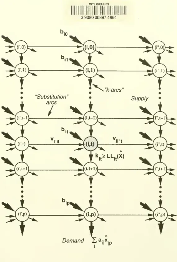
certain arcs. Fora given vectorX, consider a directed

network

G'(X) containing

nodes (i,t) corresponding toeach product i

=

1, ...,

m, and

every period t

=

, p.

The

network

contains

two

types ofarcs: (i) "substitution" arcs

from node

(i,t) to

node

(i',t) for all i

=

1

m,

i'

G

RB(i), and t

=

0, ..., p; and, (ii) "k-arcs"

from

node (i,t) to

node

(i, t+1) for all i

=

1, .... m,

and

t

=

0, ... p-1. Figure 2

shows

a portion ofthis network. In this figure, part i'

can replace part i, while part i can replace part i".

Each

k-arc

from

(i,t) to (i,t+l) has a lower

A " A

limit LLjj(X)

=

2- a^: Xj^ on its flow, i.e., the

minimum

required flow

on

this arc is LLjj(X).

Every node

(i,t), for i

=

1, ....

m

and t

=

0, .... p, has a supply ofbjj units. For i

=

1

m,

node

n

(i, _p) has a

demand (minimum

required extemal outflow) of

Z

a^jX: . (Since this

node

also

j=I n

has a supply ofbj units, its net

demand

is

Z

ajjX:

-

b- .)

j=l

A

Consider the followingy7ow/(?a.s/Z?j7/ry

problem

defined over the

network

G'(X). A

Find a feasible flow

on

G'(X) satisfying the

demand,

supply, and

minimum

arc flow constraints, orprove that no feasible flow exists.

The

mathematical formulation of this flow feasibility

problem

contains flow conservation A

equations at each node, constraints

imposing

the

minimum

flow requirements LLjj(X) on the k-arcs, and nonnegativity constraints on the flow variables. If

we

interpret the flowson the substitutionarcs as the v-variables,

and

the flows

on

the k-arcs as the k-variables, then

we

see that:

(i) the flow conservation equations at nodes (i,0) forall i

=

1

m

are the

same

as constraints

(27);

(ii) the flow conservation equationsat nodes (i,t)for all i

=

I, ...,

m, and

t

=

1 p-1, are the

same

as constraints (28);

(iii) the

minimum

flow requirements

on

the k-arcs correspond to constraints (29a); and,

(iv) for i

=

I, ...,

m,

the

demand

constraints at nodes (i,p) are the

same

as constraints (29b).

Notice that, ifthe network G'(X) has a feasible flow, then it

must

have an integral flow

(assuming all the parameters a- andb|j are integral), i.e., _{constraints (26)} are satisfied.

We

can easily incorporate upper

bounds

on the substitution variables and k-variables; these upper

A

bounds

become

arc capacities for the substitution arcs and k-arcs, respectively, in G'(X).

These observations establish the following

lemma.

Lemma

4:

A

A

given cumulative release vector

X

has a feasible completion ifand only ifthe A

corresponding network flow

problem

defined over G'(X) has a feasible solution.

A A

Note

that as

X

changes, only the

minimum

flow requirements LLjj(X) change; the

node

A

supplies and

demands

do

not change, and neither does the topology of network G'(X).

Any

algorithm used for checking feasibility of a transshipment

problem

can be used to determine if

A

G'(X) has a feasible solution.

Max-flow

algorithms are

commonly

used for this purpose.

The

max-flow problem

can be solved very efficiently in 0(INI ViEl) time,

where

INI and IE! denote the

number

ofnodes and edges in the

network

(Ahuja, Magnanti, and Orlin [1993]).

At each iteration, the bisection

method

applies the

max-flow

algorithm to verify the resource-feasibility ofthe cumulative release vector Y(z) corresponding to the current target

value z.

We

restate this iterative step (Step 1) ofthe modified bisection algorithm for solving the

APS

problem

with general precedence constraints (20) (assuming these constraints satisfy

the acyclic precedence graph property).

The

remaining steps

and

the W-evaluation subroutine are the

same

as before.

Modified

bisection

algorithm

for

the

APS

problem

with

general

precedence

constraints:

Step

1:

Search process

Construct a y-e valuation sequence S.

REPEAT

zf-

(LB +

UB)/2;

Compute W(z)

in [p,Y]; {call W-evaluation subroutine)

FOR

successive (j,t) in the sequence S,set

y:j(z)

=

max

[wjj(z),

{max

RHS

value overall precedence constraints (20) in n(j,t)}]; Construct the

network

G'(Y(z));

IF the network flow problem defined

on

G'(Y(z)) is feasible,

THEN

set

LB

<r- r(Y(z)) and (3 <- Y(z);

ELSE

set

UB

<- z and y <- Y(z);

UNTIL

(UB

-

LB)

<

e;

Let z'

e

(LB,

UB]

be the final feasible target value

when

the bisection algorithm terminates,

i.e., z' is the target valuecorresponding the last iteration in

which

the network flow problem

defined on G'(Y(z'))

was

feasible.

As

we

noted earlier,

we

can determine the appropriate

feasible v-values

from

the

maximum

flow solution corresponding to

network

G'(Y(z')).

One

disadvantage ofthis solution is that it might entail "unnecessary" substitutions, i.e., the

maximum

flow algorithm might route flows

on

certain substitution arcs

when

in fact the

problem

has an alternate

maximum

flow solution that does not use these arcs. In practice, production

managers

might prefer to reduce substitutions, as faras possible, subject to the requirement that the objective value

must

be z.

We

can incorporate this preference by solving at the

end

a

minimum

cost flow

problem

defined over the

network

G'(Y(z')).

The

node

supplies,

demands,

and arc flow lower

bounds

are as

shown

in Figure 2.

We

assign a penalty

forflow along substitution arcs, i.e., each substitution arc has a cost 5

>

per unitof flow

on

that arc.

We

seek the min-cost network flow solution that meets (orexceeds) all the

demands

using the available supplies subject tothe

minimum

flow requirements

on

the k-arcs. This min-cost flow

problem

is feasible since Y(z') is resource-feasible. Since all substitutions are

penalized equally, the optimal solution minimizes the total

number

ofparts used as substitutes.

The

model

can also incorporate part-dependent substitution penalties.

Adding

flow costs

on

the k-arcs allows

modeling

product-dependent finished

goods

inventory holding costs.

Note

there is a tradeoff

between

the value ofz

and

the (minimal) total

amount

of

substitution needed. Let

MCF(z)

denote the min-cost flow substitution

problem

on the network

G'(Y(z)), with

minimal

objective function value v(z). Since Y(z) is

monotonic

in z, as z

increases the arc lower

bounds

LLjj(Y(z)) also increase.

Thus

if Zj

<

Z2 then

MCF(Z2)

is a restriction of

MCF(zj),

sothat v(z,)

<

v(z2).

As we

increase z

we

come

closerto achieving our target service levels, but oursubstitutioncost also increases. Clearly this approach could lead to

a formal tradeoffof serviceability and substitutability.

The

following proposition establishes the validity ofthe modified bisection algorithm for

the

APS

problem.