Modelling and numerical simulation of metastable two-phase flows

HAL Id: tel-01889103

https://pastel.archives-ouvertes.fr/tel-01889103

Submitted on 5 Oct 2018

HAL is a multi-disciplinary open access archive for the deposit and dissemination of sci-entific research documents, whether they are pub-lished or not. The documents may come from teaching and research institutions in France or abroad, or from public or private research centers.

L’archive ouverte pluridisciplinaire HAL, est destinée au dépôt et à la diffusion de documents scientifiques de niveau recherche, publiés ou non, émanant des établissements d’enseignement et de recherche français ou étrangers, des laboratoires publics ou privés.

two-phase flows

Marco de Lorenzo

To cite this version:

Marco de Lorenzo. Modelling and numerical simulation of metastable two-phase flows. Mechanics of the fluids [physics.class-ph]. Université Paris-Saclay, 2018. English. �NNT : 2018SACLX029�. �tel-01889103�

Modélisation et Simulation

Numérique des Ecoulements

Diphasiques Métastables

Thèse de doctorat de l'Université Paris-Saclay

préparée à l’Ecole Polytechnique

École doctorale n°579 : sciences mécaniques et énergétiques,

matériaux et géosciences (SMEMAG)

Spécialité de doctorat: mécanique des fluides

Thèse présentée et soutenue à Palaiseau, le 28 mai 2018, par

Marco De Lorenzo

Composition du Jury : Rémi Abgrall

Professeur, Université de Zurich

Rapporteur Ray A. Berry

Distinguished Staff Scientist/Engineer, Idaho National Laboratory

Rapporteur

Daniel Fuster

Chargé de Recherches, Institut Jean Le Rond d’Alembert

Examinateur Marc Massot

Professeur, Ecole Polytechnique

Président Pierre Ruyer

Ingénieur Chercheur, Institut de Radioprotection et de Sûreté Nucléaire

Examinateur

Philippe Lafon

Ingénieur Chercheur HDR, Electricité de France

Directeur de thèse Marica Pelanti

Maître de Conférences, Ecole Nationale de Techniques Avancées

Co-encadrant

Yann Bartosiewicz

Professeur, Université Catholique de Louvain

Co-encadrant

N

N

T

:

2

0

1

8

S

A

C

L

X

0

2

9

T

he writing and completion of this Dissertation would not have been possible without the contribution, support and guidance of a few very special people. After three fantastic years spent in a new Country, working with new people and engaged on such an exciting task, the writing of the acknowledgments seems more complicated than writing the entire thesis. I will begin by thanking the jury members of my defense, then my colleagues and my friends.

I would first like to thank the reviewers of this thesis, Prof. Rémi Abgrall and Dr. Ray A. Berry, to have read and commented it. I am particularly grateful to Dr. Berry for the many technical and grammatical corrections proposed and for having traveled from the USA to attend to my PhD defense. Then, I thank the jury members, Dr. Pierre Ruyer and Dr. Daniel Fuster, for the many interesting questions and its president, Prof. Marc Massot for having coordinated the dissertation and the debate.

I would like to thank my PhD supervisor, Dr. Philippe Lafon, who has put his valuable experience and wisdom at my disposal. It has been a greatly enriching experience to me to work under his guidance. He has been supportive but he has given me the freedom to pursue various projects without objection. He has been much more than a PhD supervisor; he has been a mentor, a guidance, a colleague and a friend. His teachings have gone far beyond the two-phase flow domain, ranging from politics to demography and from history to geography and I am so grateful.

I would like to thank my co-advisors, Prof. Marica Pelanti and Prof. Yann Bartosiewicz, that helped me to learn many valuable things and to better explain and valorize my work. I must also thank my ‘extra’ co-advisor, Dr. Jean-Marie Seynhaeve, for his stimulating questions and constructive criticisms that were always more challenging.

I would like to thank my EDF colleagues: Dr. Léonard Antoinat, Dr. Frédéric Daude, David Iampietro, Dr. Hippolyte Lochon and, a CEA colleague, Pascal Galon, for the interesting debates had during the last three years but, above all, the many positive and negative criticisms that motivated me to improve my work.

I will forever be thankful to my former internship students, Michele Di Matteo and Alessandro Pantano, for their huge support. Without their daily contribution this PhD thesis would be poorer and less relevant. I tried to teach you as many things as I could; many of them were probably wrong or incomplete but I am very happy that you both are now working in the research domain. During his internship, Michele has also been one of my flatmates and I will never forget the nights and the weekends spent coding the steam-water tables and accompanied by bonne barbaque, ‘nduja, camembert and wine. This experience has strengthened our former friendship and I am very happy

beaux moments qui resteront gravés dans ma mémoire. Je remercie mon professeur d’arts martiaux, Frédéric Payet, pour sa passion et pour tout ce qu’il m’a appris dans la vie et dans le sport. Je remercie Julie Adjiman, Élodie Ricou, Francesco Bettonte, Aurélien Joly, Silun Zhang, Jingya Li, Célia Giraudeau, Jérôme Delplace pour leur amitié et leur encouragement. Je remercie très spécialement Marie Dzamba pour son soutien et sa présence inconditionnelle.

Je remercie tous mes colocs pour les beaux moments vécus ensemble: Riad Othman, Antoine Poret, Federica Tognon, Omar Hseine et, surtout, Paul Vincent, mon plus cher ami.

Ringrazio anche i miei amici di sempre: Daniele Gigliotti, Francesco Tocco, Lorenzo Niccoli, Lorenzo Petracca e Valentina Columbro. Inoltre, sono particolarmente riconoscente verso Nancy Prestanicola che mi ha reso una persona migliore ed uno studente appassionato durante i molti anni trascorsi insieme.

Infine, un ringraziamento speciale va alla mia famiglia, che è il mio punto di riferimento. Grazie per avermi educato, instruito e di avermi incessantemente incoraggiato e sostenuto in tutti questi anni. Se sono arrivato alla fine di questo cammino, è solo grazie a voi.

Peer-reviewed articles

• De Lorenzo M., Lafon Ph., Seynhaeve J.-M., Bartosiewicz Y., 2017, Benchmark of Delayed Equilibrium Model (DEM) and Classic Two-Phase Critical Flow Models against Experimental Data. Int. J. Multiphase Flow, Vol. 92, 112-30.

• De Lorenzo M., Lafon Ph., Di Matteo M., Pelanti M., Seynhaeve J.-M., Bartosiewicz Y., 2017, Homogeneous Two-Phase Flow Models and Accurate Steam-Water Table Look-up Method for Fast Transient Simulations. Int. J. Multiphase Flow, Vol. 95, 199-219.

• De Lorenzo M., Pelanti M., Lafon Ph., 2018, HLLC-type and path-conservative schemes for a single-velocity six-equation two-phase flow model: a comparative study. Applied Mathematics and Computation, Vol. 333C, 95-117.

• De Lorenzo M., Lafon Ph., Pelanti M., 2018, A hyperbolic phase-transition model with non-instantaneous EoS-independent relaxation procedures. Submitted to Journal of Computational Physics.

• Fang Y., De Lorenzo M., Lafon Ph., Poncet S., Bartosiewicz Y., 2018, An Accurate and Efficient Look-up Table Equation of State for Two-phase Compressible Flow Simulations of Carbon Dioxide. Industrial & Engineering Chemistry Research, Vol. 57(22), 7676-7691.

• De Lorenzo M., Lafon Ph., Pelanti M., Pantano A., Di Matteo M., Bartosiewicz Y., Seynhaeve J.-M., 2018, A hyperbolic phase-transition model coupled to tabulated EoS for metastable two-phase flows. Submitted to Computer & Fluids.

Presentations at international conferences

• De Lorenzo M., Lafon Ph., Bartosiewicz Y., Seynhaeve J.-M., 2016, Physical and Numerical Investigations for the Development of a New Experimental Facility for Studying Blowdown Phenomena. Proc. ICONE24, Charlotte, North Carolina, USA.

• Fang Y., De Lorenzo M., Lafon Ph., Poncet S., Bartosiewicz Y., Hakim N., 2018, Fast And Accu-rate CO2 Properties Calculation Algorithm For Massive Numerical Simulations Of Supersonic

• De Lorenzo M., Pelanti M., Lafon Ph., 2018, Non-instantaneous relaxation procedures with arbitrary equation of state for modeling liquid-vapor flows with phase transition. ECCOMAS 2018: 7th European Conference on Computational Fluid Dynamics (ECFD 7), Glasgow, UK.

Page

Table of Contents vii

List of Tables xi

List of Figures xiii

Introduction 1

Resumé en français 9

I Mathematics and physics of metastable two-phase flows 13

1 Physical features of metastability 15

1.1 Pure phase diagram . . . 15

1.2 Equations of state and thermodynamic potentials . . . 18

1.3 Saturation curve . . . 20

1.4 Stability, metastability and instability . . . 20

1.4.1 Metastable water . . . 21

1.4.2 Spinodal curve . . . 23

1.5 Metastable fluids in nature and in industry . . . 23

2 Mathematical features of two-phase flow models 25 2.1 Introduction to two-phase flows . . . 25

2.1.1 Averaging methods and diffused interface technique . . . 26

2.1.2 Computational methods for two-phase flow . . . 27

2.2 Averaged two-phase flow models . . . 28

2.3 Hierarchy of the two-phase flow models . . . 29

2.3.1 The seven-equation model . . . 31

2.3.2 The single-pressure six-equation model . . . 33

2.3.3 The single-velocity six-equation model . . . 34

2.3.4 The five-equation model . . . 35

2.3.5 The four-equation model . . . 36

2.4 Comparison of the speed of sound of two-phase flow models . . . 39

II Classical models and accurate equations of state 41 3 Steady-state metastable flows: the flashing 43 3.1 Introduction . . . 45

3.2 Mathematical Characteristics of Critical Flows . . . 48

3.3 Balance Equations of the Models . . . 49

3.3.1 Balance Equations of the Homogeneous Equilibrium Model . . . 49

3.3.2 Balance Equations of Non-Homogeneous Equilibrium Models . . . 49

3.3.3 Balance Equations of Homogeneous Non-Equilibrium Models . . . 50

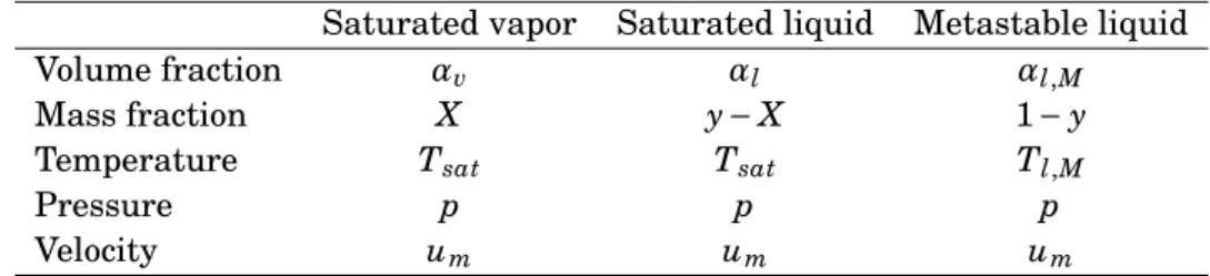
3.3.4 Balance Equations of the Delayed Equilibrium Model . . . 51

3.4 Speed of Sound of the Models . . . 52

3.4.1 Speed of Sound of the Homogeneous Equilibrium Model . . . 53

3.4.2 Critical Mass Flux of the Moody Model . . . 54

3.4.3 Speed of Sound of the Henry-Fauske Model . . . 55

3.4.4 Speed of Sound of the Delayed Equilibrium Model . . . 56

3.5 Calculation of the Critical Mass Flux . . . 57

3.5.1 Calculation of the Critical Mass Flux with Homogeneous Equilibrium Model and Moody Model . . . 57

3.5.2 Calculation of the Critical Mass Flux with Henry-Fauske Model . . . 58

3.5.3 Calculation of the Critical Mass Flux with Delayed Equilibrium Model . . . . 58

3.6 Comparison against Experimental Data . . . 63

3.6.1 Critical Two-Phase Flow Through Long Tubes . . . 65

3.6.2 Critical Two-Phase Flow Through Short Nozzles . . . 68

3.6.3 Critical Two-Phase Flow Through Slits . . . 71

3.7 Benchmark on other Critical Flow Data and Quantitative Analysis . . . 73

3.8 Conclusions . . . 75

3.9 Appendix 3.A: Condition of Critical Mass Flux of Moody Model . . . 77

4 Transient metastable flows and steam-water tables 79 4.1 Introduction . . . 81

4.2 Homogeneous two-phase flow models . . . 83

4.2.1 Homogeneous Equilibrium Model . . . 84

4.2.2 Homogeneous Relaxation Model . . . 86

4.3 Steam-water EoS for two-phase models . . . 89

4.3.1 Use of a simple caloric EoS . . . 89

4.3.2 Use of an iterative algorithm for an accurate EoS . . . 90

4.3.3 Look-up table interpolation . . . 91

4.4 IAPWS-IF97 and the representation of the liquid spinodal curve . . . 91

4.5 Look-up table method for thermodynamic properties evaluation on the e-v diagram . 95

4.5.1 Grid Construction on e-v diagram and bicubic interpolation . . . 96

4.5.2 Bicubic interpolation . . . 98

4.5.3 Derivatives calculation from bicubic splines . . . 102

4.6 Numerical simulations of steam-water transients . . . 103

4.6.1 Mass transfer for the HRM . . . 104

4.6.2 Steam-water transients . . . 105

4.6.3 Waterhammer . . . 111

4.7 Conclusions . . . 115

4.8 Appendix 4.A: HEM - Speed of sound using IAPWS-IF97 . . . 116

4.9 Appendix 4.B: HRM - Speed of sound using IAPWS-IF97 . . . 118

4.10 Appendix 4.C: Iterative algorithms for the IAPWS-IF97 . . . 119

4.11 Appendix 4.D: Derivatives of IAPWS-IF97 for the Bicubic Interpolation . . . 119

III The single-velocity six-equation two-phase flow model 123 5 Riemann solvers: a comparative study 125 5.1 Introduction . . . 126

5.2 The six-equation single-velocity two-phase flow model . . . 129

5.3 Nonconservative terms of the six-equation model . . . 130

5.3.1 Numerical treatment of the nonconservative terms . . . 132

5.4 Numerical solution methods . . . 133

5.4.1 Hyperbolic operator . . . 133

5.4.2 Pressure relaxation operator . . . 144

5.5 Test problems . . . 145

5.5.1 Water cavitation tube problem . . . 146

5.5.2 Dodecane liquid-vapor shock tube problem: shock in pure vapor . . . 148

5.5.3 Dodecane liquid-vapor shock tube problem: shock in the mixture . . . 149

5.6 Conclusions . . . 152

5.7 Appendix 5.A: Matrices of the 6-equation single-velocity two-phase flow model . . . . 154

5.8 Appendix 5.B: Model System Eigenstructure . . . 155

6 EoS-independent relaxation procedures 157 6.1 Introduction . . . 158

6.2 Six-equation single-velocity two-phase flow model . . . 160

6.3 Equations of state and thermodynamic quantities . . . 161

6.4 Physical modeling of the relaxation processes . . . 164

6.4.1 Pressure relaxation . . . 166

6.4.2 Temperature relaxation . . . 169

6.4.3 Mass transfer . . . 170

6.5.1 Hyperbolic operator . . . 173

6.5.2 Relaxation operators . . . 175

6.6 Equilibrium recovery test . . . 176

6.7 1-D numerical tests . . . 179

6.7.1 Water cavitation problem with the stiffened gas EoS . . . 180

6.7.2 Water cavitation test with the IAPWS-IF97 EoS . . . 181

6.7.3 Evaporation-condensation shock tube test with the IAPWS-IF97 EoS . . . 183

6.7.4 Evaporation shock tube test with the IAPWS-IF97 EoS . . . 185

6.8 2-D numerical test . . . 188

6.9 Conclusions . . . 189

6.10 Appendix 6.A: Semi-analytic relaxations . . . 190

6.10.1 Appendix 6.A.1: Semi-analytic temperature relaxation . . . 190

6.10.2 Appendix 6.A.2: Semi-analytic Gibbs free enthalpy relaxation . . . 191

6.11 Appendix 6.B: Irreversibility of the relaxation procedures . . . 191

6.11.1 Appendix 6.B.1: Irreversibility of the pressure relaxation process . . . 191

6.11.2 Appendix 6.B.2: Irreversibility of the temperature relaxation process . . . 192

6.11.3 Appendix 6.B.3: Irreversibility of the mass transfer process . . . 193

6.12 Appendix 6.C: Well-posedness of the relaxation procedures . . . 193

7 A six-equation single-velocity model with tabulated EoS 197 7.1 Introduction . . . 198

7.2 Six-equation single-velocity two-phase flow model . . . 199

7.2.1 Homogeneous hyperbolic portion of the model . . . 199

7.2.2 The complete model for phase transition . . . 200

7.3 Look-up table algorithm for liquid and vapor EoS . . . 201

7.3.1 The e-v diagram for water . . . 201

7.3.2 Extension to vapor metastable states . . . 202

7.3.3 A bicubic interpolation method . . . 204

7.4 Numerical solution methods . . . 206

7.4.1 Hyperbolic operator . . . 206

7.4.2 Relaxation operators . . . 208

7.5 Numerical simulations of fast depressurizations . . . 211

7.6 Conclusions . . . 215

Conclusions and perspectives 217

TABLE Page

3.1 DEM model . . . 52

3.2 Mean error for critical mass flux predictions . . . 75

3.3 Mean error for critical pressure predictions . . . 75

3.4 Standard deviation for critical mass flux predictions . . . 76

3.5 Standard deviation for critical pressure predictions . . . 76

6.1 Parameters for the Stiffened Gas EoS for liquid and vapor water (first test) . . . 181

FIGURE Page

0.1 Schematic of a Pressurized Water Reactor (PWR). . . 3

0.2 Illustration of a Loss of Coolant Accident in a PWR. . . 3

1.1 p-T diagram for pure water . . . 16

1.2 p-v diagram for pure water . . . 17

1.3 Stability, metastability and instability . . . 21

1.4 p-T diagram for pure water with metastable states . . . 22

1.5 T-v diagram for pure water with metastable states . . . 24

2.1 Two-phase flow patterns . . . 26

2.2 Hierarchy of two-phase flow models . . . 30

2.3 Celerity of two-phase flow models . . . 39

3.1 Speed of sound in vapor-liquid water of the critical models. . . 53

3.2 Schematic example of a critical trajectory in the phase space . . . 61

3.3 Benchmarks of HEM and Moody (1965) on Super Moby Dick long tubes . . . 64

3.4 Benchmarks of Henry-Fauske (1971) and DEM on Super Moby Dick long tubes . . . 65

3.5 Pressure and void fraction profiles in SMD test section: 20 bar . . . 67

3.6 Pressure and void fraction profiles in SMD test section: 120 bar . . . 68

3.7 Benchmarks of HEM and Moody (1965) on Super Moby Dick, short tubes . . . 69

3.8 Benchmarks of Henry-Fauske (1971) and DEM on Super Moby Dick, short tubes . . . . 70

3.9 Pressure and void fraction profiles in SMD short test section: 20 bar . . . 72

3.10 Benchmarks of HEM, Moody (1965), Henry-Fauske (1971) and DEM on John et al. . . 74

3.11 Benchmarks of HEM, Moody (1965), Henry-Fauske (1971) and DEM on all data . . . 77

4.1 Isobaric curve on the T-v diagram . . . 84

4.2 Mixture speed of sound for water for HEM, HRM and Wood’s relation . . . 87

4.3 Region subdivision of the IAPWS-IF97 on the p-T diagram . . . 92

4.4 Metastable domain on the e-v and p-T planes . . . 94

4.5 Trend of spinodal curves on the p-T diagram . . . 95

4.6 Isotherms on the p-v diagram . . . 96

4.7 Thermodynamic diagram e-v . . . 97

4.8 Thermodynamic diagram e-v . . . 98

4.10 Distribution of the relative error with the look-up table method . . . 101

4.11 Pressure evolution in the Bartak’s experiment . . . 105

4.12 Schematic of Super Canon experimental facility . . . 106

4.13 Assessment of HEM and HRM on a Super Canon experiment (15 MP a, 573.15 K ) . . . . 107

4.14 Comparison using different correlations forΘ (15 MPa, 553.15K) . . . 108

4.15 Comparison using different correlations forΘ (15 MPa, 573.15K) . . . 109

4.16 Comparison using different correlations forΘ (15 MPa, 593.15K) . . . 110

4.17 Pressure history of Simpson’s waterhammer experiment . . . 112

4.18 Schematic of the injection test . . . 113

4.19 Temporal evolutions at points A and B . . . 114

4.20 Magnification of the temporal evolutions . . . 115

5.1 Sketch of the phasic volume fraction increasing along z . . . 132

5.2 _{Numerical results for the water cavitation test with |u| = 2 m/s . . . 146}

5.3 _{Mesh convergence study on the water cavitation test with initial velocity |u| = 2 m/s . . . 147}

5.4 _{Efficiency study on the water cavitation test |u| = 2 m/s . . . 147}

5.5 _{Numerical results for the water cavitation test with |u| = 500 m/s . . . 148}

5.6 Numerical results for the dodecane liquid-vapor shock tube . . . 149

5.7 Numerical results for the dodecane liquid-vapor shock tube . . . 150

5.8 Benchmark test against the Saurel et al. [232] shock relations . . . 151

5.9 Numerical results for the dodecane liquid-vapor shock tube with Glimm’s method . . . . 152

5.10 Numerical results for the dodecane liquid-vapor shock tube . . . 153

6.1 Sound speed of two-phase flow models . . . 162

6.2 T-v diagram of water . . . 163

6.3 Time evolution of properties during the pressure relaxation step . . . 176

6.4 Time evolution of properties during the temperature relaxation step . . . 177

6.5 Time evolution of properties during the chemical relaxation step . . . 177

6.6 _{Evolution on the T − v diagram . . . 178}

6.7 _{Numerical results for the water cavitation test with |u| = 0.2 m/s . . . 179}

6.8 _{Numerical results for the water cavitation test with |u| = 2 m/s . . . 180}

6.9 Numerical results of the water cavitation test with the IAPWS-IF97 EoS . . . 182

6.10 Numerical results of evaporation-condensation test with the IAPWS-IF97 EoS . . . 184

6.11 Numerical results of evaporation test with the IAPWS-IF97 EoS . . . 186

6.12 Pressure field of the 2D test . . . 187

6.13 Chemical disequilibrium field of the 2D test . . . 188

6.14 Trend of the partial derivatives ∂F p i ∂yj(y) . . . 194

6.15 Trend of the partial derivatives ∂F T i ∂yj(y) . . . 194

7.1 Liquid and vapor water on the e-v diagram . . . 202

7.2 Phasic pressures, temperatures and speeds of sound on the e-v diagram. . . 203

7.4 Grid of nodes in the physical domain and in the transformed one . . . 205

7.5 Schematic of Super Canon experimental facility . . . 210

7.6 Pressure evolution in the Bartak’s experiment . . . 211

7.7 Assessment on a Edwards-O’Brien experiment (1500 P sia, 544 K ) . . . 213

M

etastable two-phase flows are involved in many industrial fields as well as in natural phenomena. In the nuclear energy industrial domain, metastable two-phase flows should be taken into account in the study of hypothetical safety accidents. Within Pressurized Water Reactors (PWRs), under nominal conditions, the coolant is a single-phase liquid water, which may transform into a two-phase mixture during accidental transients. Moreover, liquid and vapor may be in thermodynamic disequilibrium, thus, one or both phases are in metastable conditions.

In the nuclear domain, as well as in other industrial contexts, the correct simulation of those flows is of paramount importance for enhancing the safety of the system. In fact, numerical simulations are expected to provide accurate information about the mechanical efforts both on the nuclear fuel and other reactor components. Nevertheless, the analysis of the metastable two-phase flows is very challenging, and the complexity of simulating two-phase flows is higher compared to single-phase flows. In fact, for the simulation of metastable two-phase flows, there are three main difficulties: (i) the presence of a continuously moving interface that separates the two fields, (ii) the interphase transfers, and, (iii) the compressibility of both phases.

The separating interface is the locus of the discontinuities in the fluid properties. In the case of phase-transitions, this interface may also disappear due to the complete water vaporization or condensation. This feature additionally increases the complexity of modeling these phenomena.

At the interface, mass, momentum and energy exchanges take place. In phase transitions the exchanges are driven by complex mechanisms and by the thermodynamic disequilibrium between the phases. Those interfacial exchanges strongly affect the transport phenomena.

For a complete description of certain phenomena, phases must be considered as compressible fluids. On one hand, this choice is necessary for representing wave motion phenomena. On the other hand, it renders the numerical modeling even more difficult because it introduces a strong coupling between the various physical aspects as convection, wave propagation and interphase transfers, requiring appropriate methods for their mathematical solvability.

From an industrial point of view, currently, for the safety analysis of PWRs, those complex flows are described using simple models. But they are not altogether satisfactory because they do not take into account the thermodynamic disequilibrium between liquid and vapor water phases. To improve the accuracy of the numerical simulations of nuclear safety accidents, a more complete methodology is desired.

Today several computational codes are able to take into account the presence of metastable phases [24, 203, 220], however, most of them are based on an ill-posed mathematical model [254]. In the last two decades, more advanced models for metastable two-phase flows have appeared

[200, 231, 233, 283]. These are mathematically more consistent than the metastable models of the past since they have the very important feature of being hyperbolic. In nuclear industry, the transition towards these hyperbolic models has recently started [64, 221] and this thesis belongs to this path.

The purpose of this Ph.D. thesis is to develop a modern and time-efficient model for the analysis of metastable two-phase flows, and to couple it with realistic energy and mass transfer terms, together with accurate water properties.

To achieve that, we followed a progressive path. It starts with the use of classical two-phase flow models and accurate thermodynamic properties of water. Then, it focuses on the numerical aspects of a more elaborate two-phase model for metastable flows. And, finally, it couples the accurate thermodynamic methods to the elaborate two-phase flow model.

The final product of this work is a hyperbolic model for metastable two-phase flows that uses novel techniques for the calculation of interfacial transfers and up-to-date algorithms for steam-water properties. Moreover, it is computationally affordable for use in industrial configurations.

These novel techniques for the calculation of interfacial transfers are the main scientific con-tribution of this Ph.D. thesis. They allow combining today’s state-of-art in numerical modeling with up-to-date thermodynamics for real fluids. Furthermore, this methodology is time-efficient for industrial purposes.

Given the specificity of the phenomena analyzed in this thesis, the focus is on liquid and vapor water in phase transitions. However, the modeling and the numerical procedures here developed are general and may apply to different contexts.

Industrial context

This thesis, realized at the R&D department of EDF (Électricité de France), aims at studying new modeling and simulation approaches for the analysis of accidental transients occurring in nuclear power plants. EDF owns many Pressurized Water Reactors (see Fig. 0.1), therefore, the accidental scenarios studied in this work are the Loss of Coolant Accident (LOCA), waterhammers and steam explosions.

The LOCA is a hypothetical scenario and is one of the Design Basis Accidents (DBA) of nuclear power plants. It represents a sudden rupture of the primary fluid flow circuit and its depressurization (see Fig. 0.2). According to the primary system breach size, we refer to Large-Break LOCA, Small-Break LOCA or to slits. The first two represent severe hypothetical accidents of nuclear power plants. In such scenarios, the water of the primary system comes out through the break and vaporizes. This complex accident involves many physical phenomena and various components of the nuclear power plant.

In this thesis, the attention is only drawn to the two-phase phenomena at the breach, for both fast transient and stationary aspects. For the stationary aspects, Large-Break LOCA, Small-Break LOCA and slits are analyzed, whereas, for the case of the fast depressurization, the primary circuit is considered to have a full circumferential break (also called double-ended guillotine break).

FIGURE0.2. Illustration of a Loss of Coolant Accident in a PWR. Source: [257].

As concerns the fast transient aspects, if a rupture suddenly occurs in the primary system of a PWR, a depressurization wave originates at the breach and propagates upstream into the circuit. When it arrives into the reactor pressure vessel, it hits the core and it could mechanically damage the nuclear fuel and the safety and control equipment (control rods, etc.). An accurate analysis of the rarefaction wave, and of the fluid-structure interaction, can provide more precise information about the mechanical effects the core components are subjected to. At EDF, currently, these simulations are performed with the EUROPLEXUS code using an equilibrium model [105]. EUROPLEXUS code [101] is owned by the Commissariat à l’Energie Atomique et aux Energies Alternatives (CEA) and

the Joint Research Centre (JRC) of the European Union.

For the quasi-stationary aspects, it is important to evaluate the discharge rate of the coolant inventory through the breach because it influences the depressurization rate of the primary system, the pressurization of the reactor containment, etc. Establishing an accurate evaluation of the coolant discharge rate at the breach allows a better design of the safety systems of the nuclear power plant.

The other fast transients we are interested in are the waterhammers and the steam explosions. Waterhammer is a pressure surge occurring in the circuits of the power plant. This wave propa-gation phenomenon can be triggered by the sudden closure/opening of a valve, by condensation of vapor pockets, etc. Steam explosion is the interaction between two components at very different temperatures. Specifically, the temperature of the hot component is higher than the saturation temperature of the cold one. In the nuclear industry, steam explosion may occur during a severe reactor accident when the molten fuel comes into contact with the coolant water or, in a mildly form, during a Reactivity-Initiated Accident (RIA).

The common feature of all these phenomena is the presence of two-phase water in which phases may be in thermodynamic disequilibrium. Then, phases can be in metastable states, that means, the persistence of a phase into the stability domain of another phase. Furthermore, except for the analysis of the stationary flow at the breach, all the others are wave dominant phenomena in two-phase water.

Modeling approach

The analysis of the physical phenomena can be carried out by means of an empirical, mathematical or a hybrid approach. For the metastable two-phase flows, an empirical approach is necessary for the understanding of the complex interfacial mechanisms or the thermodynamic properties of real fluids. But the drawbacks of a full empirical approach stems in its narrow validity range and in the difficulty to describe the spatial and time evolution of the flow.

On the contrary, mathematical modeling helps to generalize the two-phase flows and allows treatment of a large number of physical phenomena using the same numerical tools. For instance, the same system of equations can be used to describe solid explosives, shock propagation into solid alloys, fast liquid-vapor phase transition, etc. But a methodology fully based on a mathematical approach is not able to correctly take into account some specific phenomena or the accurate fluid properties.

To balance the drawbacks of those approaches, a hybrid empirical-mathematical approach is used in this work. The mathematical modeling of the two-phase flows is the basis of our approach, however, water properties and interfacial exchanges are based on empirical laws. These laws are already present in the literature and are based on experimental data.

The system of equations analyzed in this work are the Homogeneous Equilibrium Model (HEM) [136], the Homogeneous Relaxation Model (HRM) [28] and the single-velocity six-equation two-phase flow model [234].

nonconservative formulations give incorrect shock solutions. Then, these systems of governing equations must be closed with an Equation of State (EoS) to calculate the thermodynamic properties as a function of the system conservative variables.

For water, because accurate analytical EoS for this purpose are not available yet, we adopt an efficient and very accurate algorithm to calculate water properties when the independent variables of the EoS are the density and the specific internal energy. This algorithm is based on the IAPWS-IF97 EoS formulation [273] that is very accurate and able to account for metastable states. The water properties described by this EoS are stored on a tabulated e − v diagram of water. Then, a bicubic interpolation is performed on this domain in order to accurately calculate the thermodynamic properties.

For the HEM, liquid and vapor are at full equilibrium then they are at saturation condition, therefore, during a phase transition, mass and energy transfers are dictated by the equilibrium conditions. For the HRM, the liquid is metastable and the vapor is at saturation, then the mass transfer must be modeled separately using an appropriate phase transition model. The single-velocity six-equation two-phase flow model describes the case of phases at single-velocity equilibrium but full thermodynamic disequilibrium for which the mass and energy transfer need to be defined. For both the hyperbolic transport equation and for the mass-energy exchange terms, we use the steam-water look-up method mentioned above.

To ascertain the correctness of our algorithms, several verifications have been systematically performed. The steam-water look-up method has been compared to the original IAPWS-IF97 showing a very low numerical error in terms of pressure, temperature and speed of sound. The numerical schemes for the hyperbolic systems have been verified comparing them to exact solutions, when available. The equilibrium states of the relaxation algorithms have been compared to the equilibrium conditions given by the IAPWS-IF97. Finally, to show the physical consistency of the numerical procedures and of the modeling approach, several validations have been done against the available experimental data.

Outline of the thesis

The thesis is composed of seven chapters divided into three parts. Four chapters are articles published or under review, therefore, a simple and didactic part was added to introduce the reader to the metastable two-phase flows. This is done in Part I which is composed of two chapters. Chapter 1 introduces elementary concepts of the thermodynamics of real fluids, phase diagrams, equations of state and stability-metastability-instability. Chapter 2 describes the mathematical aspects of the two-phase flows, the necessity of averaging transport equations, the mathematical characteristics of two-phase flow models and the existence of a hierarchy of these models based on the equilibrium assumptions.

a brief introduction. The order of the chapters represents the chronological order of the papers, which also shows the research path followed during the Ph.D. thesis. Each chapter represents a supplementary step towards a complete and coherent analysis of the metastable two-phase flows. The introductions that precede each chapter serve to describe the industrial needs of each work and show the links with the previous and next chapters.

Part II discusses the stationary and transient metastable flows using classical two-phase flow models and state-of-art equations of state. It is composed of two chapters, representing research articles published in the International Journal of Multiphase Flow.

Chapter 3 is about the stationary metastable two-phase flow at the breach in the event of a LOCA. Here, we compare Delayed Equilibrium Model (DEM), Homogeneous Equilibrium Model, Moody (1965) [184] and Henry-Fauske [125] models to experimental data containing a sample range in excess of 450 conditions to determine an appropriate benchmark. This analysis has been carried out for both critical mass flux and critical pressure evaluations.

Chapter 4 deals with the fast transient metastable two-phase flows as rapid depressurizations, waterhammers and steam explosions. The aim of this paper is to show an efficient and very accurate

algorithm to calculate water properties when the independent variables are the density,ρand the

specific internal energy e. For a given thermodynamic pair (ρ, e), we wish to obtain the corresponding

pressure, temperature and speed of sound. The main purpose is to couple this algorithm to two-phase flow models in their conservative form. To reach this goal, thermodynamic properties shall be tabulated on the e-v thermodynamic diagram. These developments are based on the recent works of Kunick et al. [133]. The obtained algorithm is then coupled to two common two-phase flow models, the Homogeneous Equilibrium Model and the Homogeneous Relaxation Model, and their numerical simulations are compared to experimental data showing the very good performance of our computational approach.

Part III is devoted to the single-velocity six-equation two-phase flow model and its use for the numerical simulation of fast transients. It is composed of three chapters that describe the evolution in numerics and modeling for the final use of this two-phase flow model, fully coupled to the proposed steam-water tables, for the simulation of fast depressurizations.

In Chapter 5 we make a comparison of different numerical schemes for several test cases, including cavitation problems and shock tubes. The main difference between these schemes stems from their differing numerical treatments of the nonconservative terms. Further, an efficiency study for first and second order schemes is also presented. Attention is drawn to the numerical resolution of the homogeneous portion of this model, hence, the equation of state used throughout this chapter is an analytic one allowing comparison of the numerical results to the exact solutions.

In Chapter 6 new non-instantaneous EoS-independent relaxation procedures are proposed for the treatment of phase transition cases. These new procedures are tested from both thermodynamic and numerical points of view. In particular, we show that, starting from a metastable mixture, they are able to recover the correct full equilibrium state.

We also show that these new relaxation procedures converge to instantaneous equilibrium simulations when the characteristic equilibrium recovery times tend to zero. Here the single-velocity six-equation two-phase flow model is coupled to the IAPWS-IF97 equation of state. This chapter is

coupling of the look-up table method to the single-velocity six-equation model for the calculation of phasic properties. Here, the hyperbolic solver of the six-equation model as well as the non-instantaneous EoS-independent relaxation procedures use the steam-water tables for an accurate description of fast depressurizations.

C

ette thèse de doctorat s’intéresse aux écoulements diphasiques métastables typiques de certains transitoires accidentels qui pourraient intervenir dans les centrales nucléaires. Ces phénomènes sont difficiles à traiter en raison de la complexité topologique de l’écoulement, des transferts entre phases et du couplage fort entre les caractéristiques thermodynamiques et les aspects mathématiques. Les méthodes aujourd’hui en usage dans l’industrie ne décrivent pas complètement la complexité de ces écoulements car elles s’appuient sur des modèles trop simples. En fait ces méthodes ne prennent pas en compte le déséquilibre thermo-chimique entre l’eau liquide et sa vapeur. Par ailleurs, les méthodes hyperboliques proposées récemment dans la littérature pour la simulation des écoulements métastables ne peuvent pas être appliquées dans l’industrie car elles utilisent des lois d’état simples qui ne sont pas adaptées pour les calculs industriels. Le but de cette thèse est de développer une nouvelle approche qui couple les méthodes hyperboliques modernes à des équations d’état précises.

Le premier chapitre est consacré à une introduction à la physique et à la thermodynamique des fluides métastables. On présente d’abord les concepts élémentaires à propos du diagramme de phase en se concentrant sur le mélange liquide-vapeur. Puis les concepts de degrés de liberté et de potentiels thermodynamiques sont introduits. Pour aborder le concept de métastabilité c’est l’approche phénoménologie basée sur la thermodynamique des milieux continus qui est utilisée ici. Enfin, l’importance de la métastabilité est discutée pour différents phénomènes existants dans la nature ou dans l’industrie. Bien que les analyses conduites dans ce chapitre soient valables pour n’importe quel fluide, une attention particulière est bien sûr accordée à l’eau.

Le second chapitre est dédié à introduire les principaux concepts mathématiques qui seront nécessaires par la suite. Tout d’abord on introduit les principales caractéristiques des écoulements diphasiques. Les complexités physiques et mathématiques des écoulements diphasiques sont notam-ment discutées ainsi que les conséquences en terme de difficultés numériques pour la simulation de tels écoulements. Dans ce cadre, les équations de conservation des écoulements diphasiques sont le plus souvent moyennées. D’autre part, de nombreuses techniques numériques existent si bien qu’il est nécessaire de clairement préciser quelles approches seront utilisées afin de bien définir le contexte numérique de la thèse. Ensuite on donne des éléments d’information mathématiques pour les écoulements diphasiques compressibles et leurs équations d’état et on décrit les modèles d’écoulements diphasiques les plus communs ainsi que la hiérarchie existant entre eux en fonction du degré de déséquilibre autorisé entre phases. Les différentes formulations de la vitesse du son associée à ces modèles sont finalement analysées.

sûreté des réacteurs PWR en cas d’APRP dépend de la capacité à évaluer le débit de fuite du liquide de refroidissement à la brèche. A cause de la grande différence de pression entre l’eau primaire et le bâtiment réacteur, le débit massique est bloqué à la brèche. Sous ces conditions, les déséquilibres mécanique et thermodynamique entre phases ne sont pas assurés. Une théorie générale pour le débit critique diphasique n’est pas encore disponible. Cependant, des modèles sont capables de fournir des évaluations précises à la fois des débits critiques et des pressions critiques, comme le modèle DEM (Delayed Equilibrium Model) dont il est principalement question ici. On montre comment intégrer le système d’équations du modèle DEM en couplant une méthode de Runge-Kutta classique à l’algorithme Possible-Impossible pour l’écoulement, ce qui donne une procédure de résolution assez simple sans recourir à des schémas numériques sophistiqués. Puis les quatre modèles DEM, HEM (Homogeneous Equilibrium Model), Moody (1965) et Henry-Fauske (1971) sont comparés aux données expérimentales disponibles. Plus de 450 conditions expérimentales sont ainsi utilisées couvrant notamment des configurations différentes de type «tuyau long», «tuyau court» et «fissures». Le modèle DEM donne finalement les meilleurs résultats.

Le quatrième chapitre est consacré aux écoulements transitoires métastables et aux tables thermodynamiques pour l’eau et sa vapeur. En effet, le système des équations de conservation doit être fermé à l’aide d’une équation d’état afin de calculer la pression en fonction des variables conservatives. Pour l’eau, des équations d’état analytiques suffisamment précises ne sont pas encore disponibles. On propose ici un algorithme efficace et précis pour calculer les propriétés de l’eau quand les variables indépendantes de la loi d’état sont la densité et l’énergie interne spécifique. Cet algorithme utilise la formulation IAPWS-IF97 pour la loi d’état de l’eau et sa vapeur, et une méthode de tabulation s’appuyant sur une interpolation bicubique. La métastabilité dans le domaine liquide est étendue jusqu’à la spinodale. La loi d’état ainsi définie est couplée à deux modèles diphasiques classiques : le modèle HEM (Homogeneous Equilibrium Model) et le modèle HRM (Homogeneous Relaxation Model). Ils sont utilisés pour simuler des problèmes de dépressurisation rapide, de coups de bélier et d’injection d’énergie. Les comparaisons avec des données expérimentales montrent les bonnes performances des algorithmes proposés.

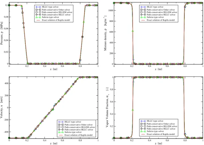
Le cinquième chapitre présente une étude comparative de différents solveurs de Riemann dans le cadre de l’intégration du modèle diphasique à six équations et une vitesse avec relaxations instantanées. La littérature montre l’efficacité de ce modèle pour la simulation d’écoulements complexes incluant des processus de vaporisation et de cavitation. On présente ici l’analyse de différents schémas numériques pour ce modèle en se concentrant sur l’intégration des termes non-conservatifs présents dans les équations d’énergie phasiques. Deux nouvelles méthodes sont proposées : un path-conservative schéma de type HLLC basé sur la théorie de Dal Maso – Le Floch – Murat et un schéma de type HLLC généralisé basé sur un solveur de Riemann de type Siliciu. Ce dernier schéma présente l’importante propriété de préserver la positivité aux états intermédiaires des quantités conservées. On utilise aussi deux autres schémas proposés dans la littérature qui sont dérivés des solveurs de Riemann Osher et HLLEM. On compare ces schémas sur différents cas-tests dont des cas de cavitation et des tubes à choc. Les résultats numériques montrent que les différentes méthodes qui correspondent à différents traitements numériques des termes non conservatifs donnent des résultats similaires et précis sauf, comme attendu, pour les chocs diphasiques aux très

procédures de relaxation instantanées et indépendantes de la loi d’état. Dans ce cadre, les deux phases initialement à différentes pressions, températures et potentiels chimiques sont supposées être amenées vers les conditions d’équilibre grâce à trois processus successifs de relaxation. Tout d’abord, un processus mécanique s’applique à la relaxation des pressions phasiques, puis un processus thermique pilote le transfert de chaleur sensible entre les phases à différentes températures et enfin un processus chimique est responsable du transfert de masse. Le modèle à six équations et une vitesse est composé de six équations avec termes source qui autorisent la description de mélanges avec déséquilibre thermodynamique complet. La partie homogène du système d’équations est résolue à l’aide d’un schéma volume fini à l’ordre deux qui utilise un solveur de Riemann de type HLLC. Les termes source qui modélisent les processus de relaxation sont intégrés séparément sous la forme de trois systèmes d’équations différentielles ordinaires. La contribution majeure de ce travail concerne la capacité de décrire le temps de retard pour le retour à l’équilibre, l’indépendance par rapport à la loi d’état de l’ensemble du processus numérique et la possibilité de prendre en compte la morphologie de l’écoulement en utilisant l’aire interfaciale entre phases.

Le septième chapitre est consacré à l’application des différents développements des chapitres précédents : modèle diphasique à six équations et une vitesse, tables thermodynamiques métastables pour l’eau et sa vapeur, solveurs de Riemann et enfin nouvelles procédures de relaxation. Le cas test retenu est représentatif des problèmes de dépressurisation rapide comme en situation d’APRP. Le modèle fournit des résultats en très bonne correspondance avec les données expérimentales notamment en ce qui concerne les effets métastables.

Le produit final de ce travail de thèse est un nouveau modèle pour l’analyse industrielle des écoulements diphasiques métastables qui associe de nouvelles techniques pour le calcul des trans-ferts entre les phases et des propriétés de l’eau et de sa vapeur. De plus, cette approche est d’un coût abordable pour les configurations industrielles. Les méthodes développées dans cette thèse ont été systématiquement vérifiées avec des solutions exactes et validées en utilisant des données expérimentales de la littérature

Mathematics and physics of

metastable two-phase flows

C

H

A

P

1

P

HYSICAL FEATURES OF METASTABILITY

T

his first chapter is devoted to a bibliographic introduction to thermodynamics and to the

physics of metastable fluids. It starts with elementary concepts about the phase diagram of a pure fluid focusing on the liquid-vapor mixtures. It introduces also the basic thermodynamic concepts of degrees of freedom and the thermodynamic potentials. Then the equations of state are briefly discussed and the concepts of stability and equilibrium are introduced. About the metastability, the so called phenomenological approach is used here because it is based on the continuum thermodynamics. Then the chapter ends with a discussion on the importance of the metastability in both nature and industry. Even though the thematics treated in this chapter are valid for any pure fluid, particular attention will be devoted to water due to the industrial context of this thesis.

1.1

Pure phase diagram

A pure phase can exist under different states of aggregation. For instance water, at atmospheric pressure, according to its temperature, can be solid, liquid or vapor. A phase diagram allows to schematize such information. In Fig. 1.1, the p-v-T and the p-T diagrams for pure water are reported. Referring to Fig. 1.1(b), the red lines are the loci of two-phase equilibrium and delimit the stability domains of the three phases.

More precisely, the melting curve indicated by T M continues indefinitely to the highest pressure. Conversely, the vapor-liquid curve indicated by TC terminates at the critical point C. Beyond this point, we speak about the supercritical domain where fluctuations becomes important and vapor and liquid can be no longer distinguished, therefore, we refer at it as supercritical fluid.

Water is a very particular matter with many anomalies. For instance, the negative slope of the melting curve means that the density of the solid is lower than the one of the liquid. Or the liquid density maximum at 277.13 K , that is one of the most famous anomalies of water [255]. At low

(a)

(b)

FIGURE 1.1. (a) p-v-T and (b) p-T diagrams for pure water. Sources:

http://sounak4u.weebly.com/properties-of-pure-substance.html and https://commons. wikimedia.org/wiki/File:Clausius-Clapeyron_phase_diagram.png.

when the temperature decreases [73, 210], that is untypical for a liquid. Further, the specific heat of water is extremely elevated. Many other unusual properties make water a complicate matter in thermodynamics, therefore, to well approximate its behavior, complex equations of state are needed. For this reason, this thesis fully relies on the state-of-art equations of state IAPWS-95 [272] and IAPWS-IF97 [273], based on a large database of experimental data.

FIGURE1.2. p-v diagram for pure water. Realized using IAPWS-IF97 EoS.

triple point T, where the three phases coexist and the fluid properties are [272]:

T_{tr= 273.16 K,} p_{tr= 0.6117 · 10}−3MP a.

The properties at the triple point are very well known. Since the 5thInternational Conference on

the Properties of Steam in London in 1956, it has been taken as reference state, thus the specific internal energy and the specific entropy of the saturated liquid triple point are set equal to zero:

e_{tr= 0 kJ/k g,} s_{tr= 0 kJ/k g/K.} The second one is the critical point C [272]:

Tcr= 647.096 K, pcr= 22.064 MPa, ρcr= 322 k g/m3.

Concerning the degrees of freedom (Gibbs rule) of the matter, when only a single phase is present, the internal equilibrium is said to be divariant, that is the degrees of freedom are two. This means that to know the properties of the matter, two variables must be fixed, for instance pressure and temperature. When two phases are present and are in equilibrium (along the red lines of Fig. 1.1(b)), the system in univariant, that is, one degree of freedom, thus pressure and temperature are correlated. The critical and the triple points are fixed once for all, then the system is said to be invariant.

Given that this thesis deals with metastable fluids, as we will see in Chapter 2, phases can be divariant also in a mixture when phases are not in equilibrium.

The study of the liquid-vapor mixtures lying along the vaporisation curve, going from the triple point to the critical point, is the main topic of this thesis. For completeness, let us say also that the vaporization curve is also called in the literature as the saturation curve, the vapor-pressure curve or the coexistence curve. This curve is depicted in Fig. 1.2 on the p-v plane, where the vaporisation

curve becomes a dome. In Fig. 1.2, two isotherms are also shown: the one corresponding to 623.15 K and the critical one. Here we can see that in the saturation dome, when phase are in thermal equilibrium, the isotherms are also isobars due to the univariance of the equilibrium two-phase mixtures discussed above. Nevertheless this is not the case for mixtures of metastable phases.

Regarding the critical isotherm, it is the one that admits a horizontal tangent and an inflexion point, defining the end of the vaporisation curve. Mathematically, at the critical point:

µ∂_p ∂v ¶ T= 0, µ∂2_p ∂v2 ¶ T= 0, (1.1) and µ∂_T ∂s ¶ p= 0, µ∂2_T ∂s2 ¶ p= 0. (1.2) On the p − T diagram, the liquid-vapor transitions are accompanied by volume (but also entropy) discontinuities. For this reason they are usually called first order phase transitions1. The latter is a segment on the p-v diagram and is called binodal curve. The liquid-vapor transition at the critical point is not accompanied by a volume or entropy discontinuities but is called second order phase transitions because of the mathematical characteristic of this point (see Eqs. (1.1) and (1.2)). In this thesis we are mainly focused on first order phase transitions.

1.2

Equations of state and thermodynamic potentials

From the previous section it was stated that a single-phase system has two degrees of freedom. Therefore one needs to know two variables, together with a corresponding equation of state, to identify the thermodynamic state of the system.

The equation of state is a thermodynamic equation relating state variables and describes the physical conditions of the matter. This thermodynamic relation is usually constructed using thermodynamic potentials describing the equilibrium behavior of a system. They are: the internal energy, e, the Helmholtz free energy, f , the enthalpy, h, and the Gibbs free energy, g. The latter will be also called Gibbs free enthalpy. These potentials are related each other by the following algebraic relations:

f = e − Ts, h = e + pv, g = h − Ts,

(1.3)

where s is the specific entropy. Thanks to the thermodynamic potentials, the complete EoS take the form of

e(s, v), f (T, v), g(T, p), h(s, p). (1.4)

Here the complete EoS are expressed in natural variables, that is, a set of appropriate variables that allow to compute the other thermodynamic potentials by partial differentiation. Therefore, no

1_{Ehrenfest proposed that the order of the transition is given by the lowest-order derivative of the Gibbs energy that is}

other relations are needed to describe the thermodynamic behavior of the matter. In Chapter 2 we will see that compressible flow models require an equation of state in the form

p(ρ, e). (1.5)

This is an incomplete EoS and needs additional relations to define, for instance, the temperature [63, 181]. Moreover, an incomplete EoS can not determine a corresponding complete EoS [181]. In this thesis, the incomplete EoS are replaced by iterative or a look-up table inversion of a reference complete EoS.

Referring to the thermodynamic potentials, their differentials are: d e = Tds − pdv,

d f = −sdT − pdv, dh = Tds + vd p, d g = −sdT + vd p.

(1.6)

The first is called Gibbs relation and is the fundamental equation of classical thermodynamics. In this context, Legendre transformations are a useful tool to pass from a potential to another one, see [4, 285] for further details. From those, together with the symmetry property of the second derivatives, one can obtain the Maxwell’s relations:

µ∂_T ∂v ¶ s= − µ∂_p ∂s ¶ v= + ∂2_e ∂s∂v, µ_∂T ∂p ¶ s = + µ_∂v ∂s ¶ p = + ∂ 2_h ∂s∂p, µ∂_s ∂v ¶ T= + µ∂_p ∂T ¶ v= − ∂2_f ∂T_∂v, µ∂_s ∂p ¶ T = − µ∂_v ∂T ¶ p = − ∂ 2_g ∂T∂p. (1.7)

These relations will be extensively used for the calculation of the partial derivatives ¡∂

∂v ¢ e and ¡∂ ∂e ¢

v needed for the water properties tabulation on the e-v plane. And they will be also useful to

express more easily certain derivatives in the analysis of the relaxation of the thermodynamic disequilibrium.

Let us define also some thermodynamic properties that are used in the following. The specific heats at constant volume and pressure are

cv= µ∂_e ∂T ¶ ρ= T µ∂_s ∂T ¶ ρ , cp= µ∂_h ∂T ¶ p= T µ∂_s ∂T ¶ p . (1.8)

The isothermal and isentropic compressibility factors are kT= 1 ρ µ∂ρ ∂p ¶ T , ks= 1 ρ µ∂ρ ∂p ¶ s . (1.9)

The coefficient of thermal expansion is

β= −ρ µ_∂ρ ∂T ¶ p . (1.10)

The previous properties are also called direct measurable quantities and may be related by two identities ks kT = 1 − β2_T ρcpkT = cv cp . (1.11)

Alongside with the phasic measurable quantities, two dimensionless parameters will be also used in

the following. The adiabatic exponentγand the Grüneisen coefficientΓ:

γ= 1 ρp µ∂2_e ∂v2 ¶ s = 1 p ks , Γ =1 ρ µ∂_p ∂e ¶ ρ= β cvkT . (1.12)

A paramount variable in compressible flows is the isentropic speed of sound. It is defined as

c = s 1 ρks . (1.13)

1.3

Saturation curve

Along the saturation curve (or vaporization curve), the phase are in full thermodynamic equilibrium: pl= pv,

Tl= Tv,

gl= gv,

(1.14)

where subscripts l and v indicate, respectively, the liquid phase and the vapor one, and where g denotes the Gibbs free enthalpy. The conditions expressed in Eq. (1.14) are also called Maxwell criterion [179].

Since the system is univariant, a dependency psat(T), or Tsat(p), exists. For instance, to construct

the relation psat(T) we apply the Gibbs-Duhem equation (see Eq. 1.6) between the two saturated

states. Since it is an isotherm, this reduces to: gv− gl=

Z pv

pl

vd p. (1.15)

Then, the saturation curve, psat(T), can be constructed by requiring the vanishing of Eq. (1.15).

Other methods exist to construct the saturation curve. However, in the case of water, the IAPWS-IF97 provides a suitable basic equation that relates saturation pressure and temperature.

1.4

Stability, metastability and instability

In this section a brief introduction to the concepts of stability, metastability and instability is given. Although it must not be considered as fully exhaustive. To learn more about this subject, the author suggests [43, 73] for a rigorous thermodynamic approach and [41] for a graphical and effective understanding.

To briefly introduce these concepts, it is useful to make the classical analogy reported in Fig. 1.3. It depicts the trend of a potential energy with respect to an arbitrary abscissa and the state of the system is represented by a sphere that can roll to a lower potential energy to reach its equilibrium.

FIGURE 1.3. Concepts of stability, metastability and instability. Source: https://en.wikipedia.org/wiki/Metastability, drawing made by Georg Wiora (Dr. Schorsch).

The red sphere represents the metastable state, the green one the instable state and the blue the stable state of equilibrium of the system. Referring to thermodynamics, the potential energy is the Gibbs free enthalpy and the abscissa could be the specific volume.

The equilibrium state of the system corresponds to the absolute minimum of the Gibbs energy [43, 73] however another minimum exist, that is a relative minimum, and is where the red sphere lies. Let us consider now a liquid-vapor phase transition. The abscissa of the metastable state is the one of the liquid that is obviously lower than the one of the vapor, represented by the blue sphere. The equilibrium phase of the system would be the vapor one, however the fluid is initially a metastable liquid. In order to reach the equilibrium, it needs to overcome an energy barrier (the bump on the top of which the green sphere is located). Then it needs a high enough perturbation.

In other words, a metastable system, when subject to small perturbation does not evolve into another state; however, when the perturbation is higher than a certain activation value, it does. On the contrary, a stable system remains in its state no matter the perturbation. Finally, the instable state evolves to another state if subject to arbitrarily small perturbations.

1.4.1 Metastable water

In this work we refer to the metastability as: the persistence of a phase into the stability domain of another phase. For instance Fig. 1.4 shows the existence of metastable subcooled vapor in the subcooled liquid domain and the metastable superheated liquid in the superheated vapor domain. Obviously, the lifetime of a metastable phase is limited since a stable phase is always going to appear sooner or later. Moreover, the deeper the metastability of a phase, the shorter its lifetime is [73, 245]. In real systems, the fluids are never pure, suspended impurities exist, the container walls have irregularities, etc. These facilitate the nucleation of a new phase preventing the fluid to reach a deep metastable state. They simply decrease the energy barrier discussed above, needed to activate the nucleation mechanisms. This means that the higher the purity of a fluid, the higher is the possibility to reach a deep metastable state.

In the case of liquid water, experimentally, one can observe the supercooled water, the superheated water and the tensile water. The first is the case of water staying in liquid form below its solidification

FIGURE1.4. p-T diagram of water. The plot has been realized using the IAPWS-IF97.

temperature, for instance [73, 138]. The second is liquid water at a temperature higher than the boiling temperature (or, equivalently, at a pressure lower than the saturation pressure) and is the case on which this work is focused on. Some experimental evidences of superheated water are reported in [8, 32, 246]. The superheated water could also reach negative pressures, that is the fluid is able to make a tensile strength on its container walls, for this reason it is also called tensile [73, 131]. The vapor can be metastable too, as in the case of the subcooled vapor, i.e. vapor at a temperature lower than the condensation one.

A good reference for the experimental procedures to obtain metastable water and their limits is [99].

There are two approaches to the phase stability: the microscopic and the phenomenological ones. The first is based on statistical mechanics. The second is based on the continuum thermodynamics and is more suitable for macroscopic systems, therefore, the more appropriate for our industrial purposes. A remarkable difference between the two approaches is that following the microscopic approach, there is not a sharp transition from metastability to instability. The spinodal is not a mathematical and physical locus, rather, an approximation.

For the phenomenological approach we start analyzing the phase stability of an isolated system. From thermodynamics, it is well known that an isolated system attains a maximum value of entropy at equilibrium [43]. Hence, the criteria for equilibrium and stability can be expressed as:

δS = 0 criterion of equilibrium,

δn

S < 0, for the smallest n at whichδn_{S 6= 0} criterion of stability,

(1.16)

where_δS and_δnS are a shorthand way of representing the terms of successive order. For instance,

for S = S(e, v): δS = µ∂_S ∂e ¶ vd e + µ∂_S ∂v ¶ e dv. (1.17)

Further developments of the last criterion of Eq. (1.16) provide two conditions which ensure the stability of a system:

cv> 0 criterion of thermal stability,

µ∂_p ∂v ¶

T

< 0 criterion of mechanical stability.

(1.18)

If both are satisfied, the system is intrinsically stable. Both the equilibrium and the metastable phase are intrinsically stable, however, the latter remains in this condition only for a finite time interval. When the thermal fluctuations and the molecular vibrations drive the system to the equilibrium conditions, provoking vaporisation (for the superheated liquid) or condensation (for the subcooled vapor), the metastable phase disappears.

1.4.2 Spinodal curve

The criterion of thermal stability shown in (1.18) is always satisfied, whereas the fulfillment of the mechanical stability criterion is not always ensured. For instance, cubic EoS, such as the van der Waals EoS, satisfy the mechanical stability condition until the so-called spinodal line. The spinodal line seems to indicate the separation between the unstable domain from the stable/metastable one, however, it is just an artifact of equations of state describing both the liquid and the vapor phase.

In equilibrium thermodynamics phase transition occurs at saturation conditions, on the contrary, in real systems an isothermal pressure change would very likely carry the state point into the metastable domain. The deeper the metastability reached, the higher is the probability for the phase change to occur. The spinodal curve is the limit beyond which phase change has already occurred.

The liquid and vapor spinodal lines connect all the minima of the isotherms (liquid spinodal) and all the maxima (vapor spinodal) closest to the associated side of the saturation curve within the saturation dome. At these minima and maxima points isotherms have zero slope (see Fig. 1.5), hence, spinodal lines mark the location from where the mechanical stability condition is violated.

Using the IAPWS-IF97 as EoS, we reveal in the following that the spinodal corresponds to positive values of the pressure until T ≈ 593.50 K. Below this temperature, the limit of mechanical stability corresponds to negative pressures. This is the domain of the tensile water [49, 73, 131, 132, 143, 170, 245, 284], however this is out of interest in this thesis.

1.5

Metastable fluids in nature and in industry

Pure water and aqueous solutions are often in metastable conditions, both in nature and industry, nonetheless, these conditions of the matter are often ignored. For this reason, this section enumerates and briefly discusses the main fields in which metastable states exist.

In geology, the water is often metastable in the soil due to capillarity [206] or in the deep earth’s crust [243]. Metastable states are common in regions of high thermal fluxes (volcanic regions and magmas [259], geysers [215], etc.), therefore, many research papers on metastability come from the geophysics and geochemistry journals. Evidently, this is not restricted to the planet Earth, in fact, metastable aqueous solutions are believed present in the hyper-arid environments of Mars [182, 183].

FIGURE1.5. T-v diagram of water. The plot has been realized using the IAPWS-IF97. Here

we can see the saturation curve, the spinodal curve ((∂p/_∂v)_T= 0) and an isobaric

curve (i.e. p = 12.7 MPa). The latter has been divided in three portions: the blue one represents the liquid states, the red one denotes the vapor states and the black dotted curve refers to the unstable states that connect the previous ones. Going rightwards along the isobaric curve, up to point (a) water is liquid in a stable state, from (a) to (b) water is a metastable liquid, from (b) to (c) the fluid is in unstable conditions, from (c) to (d) water is in metastable vapor conditions and, starting from point (d), the vapor is stable.

In biology, the metastable states, especially the supercooled ones, play a fundamental role for the life of cells, microorganisms, etc. An interesting discussion is reported in the introductory chapter of [73].

Another relevant field in which we can find metastable water is in plant physiology. In fact, an aqueous solution, called sap, becomes tensile in reaching the tops of trees. The fact that water

reaches negative pressures inside the trees is known at least from the 19thcentury [73]! Many of

the EoS for the negative pressure domain have been developed to simulate such a phenomenon. As concerns industry, metastability is often synonym of accident. In industrial processes, metastable states typically appear due to fast depressurizations or to energy injection. As al-ready discussed, the industrial context of this thesis is the one of the hypothetical nuclear accidents involving metastable two-phase flows. However, the same phenomena could be encountered in many industrial process or chemical factories. For example, in beer or sparkling drinks production sites, paper factories, in the metallurgy for cooling the melting metals, in petroleum engineering (LNG), etc.

Some of them are fully stationary as the critical two-phase flow through a safety valve or a breach of a pipe. Some others are highly non-stationary phenomena, like fast depressurizations, waterhammers or energy injection. Those kinds of phenomena are separately addressed respectively in Chapters 3 and 4.