HAL Id: hal-00297175
https://hal.archives-ouvertes.fr/hal-00297175
Submitted on 5 Dec 2005
HAL is a multi-disciplinary open access
archive for the deposit and dissemination of
sci-entific research documents, whether they are
pub-lished or not. The documents may come from
teaching and research institutions in France or
abroad, or from public or private research centers.
L’archive ouverte pluridisciplinaire HAL, est
destinée au dépôt et à la diffusion de documents
scientifiques de niveau recherche, publiés ou non,
émanant des établissements d’enseignement et de
recherche français ou étrangers, des laboratoires
publics ou privés.
shallow cumulus over land
J. Vila-Guerau de Arellano, S.-W. Kim, M. C. Barth, E. G. Patton
To cite this version:
J. Vila-Guerau de Arellano, S.-W. Kim, M. C. Barth, E. G. Patton. Transport and chemical
trans-formations influenced by shallow cumulus over land. Atmospheric Chemistry and Physics, European
Geosciences Union, 2005, 5 (12), pp.3219-3231. �hal-00297175�
Atmos. Chem. Phys., 5, 3219–3231, 2005 www.atmos-chem-phys.org/acp/5/3219/ SRef-ID: 1680-7324/acp/2005-5-3219 European Geosciences Union
Atmospheric
Chemistry
and Physics
Transport and chemical transformations influenced by shallow
cumulus over land
J. Vil`a-Guerau de Arellano1, S.-W. Kim2, M. C. Barth2, and E. G. Patton2
1Meteorology and Air Quality Section, Wageningen University, The Netherlands
2Mesoscale and Microscale Meteorology Division, National Center for Atmospheric Research, USA
Received: 5 August 2005 – Published in Atmos. Chem. Phys. Discuss.: 16 September 2005 Revised: 15 November 2005 – Accepted: 15 November 2005 – Published: 5 December 2005
Abstract. The distribution and evolution of reactive species
in a boundary layer characterized by the presence of shal-low cumulus over land is studied by means of two large-eddy simulation models: the NCAR and WUR codes. The study focuses on two physical processes that can influence the chemistry: the enhancement of the vertical transport by the buoyant convection associated with cloud formation and the perturbation of the photolysis rates below, in and above the clouds. It is shown that the dilution of the reactant mixing ratio caused by the deepening of the atmospheric boundary layer is an important process and that it can decrease reac-tant mixing ratios by 10 to 50 percent compared to very sim-ilar conditions but with no cloud formation. Additionally, clouds transport chemical species to higher elevations in the boundary layer compared to the case with no clouds which influences the reactant mixing ratios of the nocturnal resid-ual layers following the collapse of the daytime boundary layer. Estimates of the rate of reactant transport based on the calculation of the integrated flux divergence range from to
−0.2 ppb hr−1to −1 ppb hr−1, indicating a net loss of sub-cloud layer air transported into the sub-cloud layer. A comparison of this flux to a parameterized mass flux shows good agree-ment in mid-cloud, but at cloud base the parameterization un-derestimates the mass flux. Scattering of radiation by cloud drops perturbs photolysis rates. It is found that these per-turbed photolysis rates substantially (10–40%) affect mixing ratios locally (spatially and temporally), but have little effect on mixing ratios averaged over space and time. We find that the ultraviolet radiance perturbation becomes more important for chemical transformations that react with a similar order time scale as the turbulent transport in clouds. Finally, the detailed intercomparison of the LES results shows very good agreement between the two codes when considering the evo-lution of the reactant mean, flux and (co-)variance vertical profiles.
Correspondence to: J. Vil`a-Guerau de Arellano
1 Introduction
Shallow cumulus (Cu) clouds over land are a manifesta-tion of convecmanifesta-tion in the atmospheric boundary layer (ABL). Their formation and evolution depend strongly on the parti-tioning between the sensible- and latent-heat fluxes, the wind shear and the vertical structure of the thermodynamic state variables. Because the structure of the boundary layer with shallow cumulus differs from the clear boundary layer, the dynamics driven by the presence of Cu leads to variations of the boundary layer characteristics, which also determines the evolution and distribution of atmospheric reactive com-pounds. Shallow cumulus clouds generally form in synopti-cally high pressure regions which are conducive to the forma-tion and accumulaforma-tion of both passive and photochemically generated pollutants in the boundary layer because of the low wind speeds, the intensification of capping inversions, and high insolation. As a consequence, shallow Cu can affect the variability of chemical species in four ways: (a) the en-hancement of vertical transport of the chemical species, (b) the turbulent mixing of atmospheric compounds, (c) the per-turbation of ultraviolet radiation, and therefore of photodis-sociation rates, below, in and above the clouds and (d) the chemical reactions occurring within the cloud droplets. In this study, we focus on the first three of these effects.
Although shallow Cu clouds are a common feature in at-mospheric boundary layers over land, little is known about their role on the transport, mixing, and photodissociation of chemical compounds. Shallow cumulus have the potential to enhance vertical transport of atmospheric compounds such that the compounds reach higher altitudes. The vertical trans-port is dependent on the strength of the clouds and on the temperature capping inversion. Field observations (Ching and Alkezweeny, 1986; Ching et al., 1988; Baumann et al., 2000; Angevine, 2005) have shown that the presence of shal-low cumuli leads to a reduction of the pollutants in the sub-cloud layer due to the enhanced vertical transport by cumulus clouds.
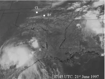
Fig. 1. GOES-8 satellite visible image at 11:45 LT (17:45 UTC) 21 June 1997. The image shows shallow cumulus fields above the radiosonde sites C1 and B5. The locations of the central facility of the Southern Great Plains (SGP) site C1 (36.605◦N, 97.485◦W, el-evation 315 m) of the Atmospheric Radiation Measurement (ARM) program and the radiosounding B5 (35.969◦N, 95.856◦W, eleva-tion 345 m) are shown.
In these cloudy boundary layers, highly turbulent regions are localized in the cloud updraft whereas the compensat-ing subsidence regions are characterized by less turbulent downward motions. As a result, reactive species may be-come segregated such that turbulent mixing controls the reac-tivity of second-order chemical reactions (Schumann, 1989; Molemaker and Vil`a-Guerau de Arellano, 1998). This lim-itation of reactivity is particularly important if the chemical time scales are of similar order to the turbulent transport time scale.
Finally, clouds disrupt the ultraviolet radiation field by per-turbing the contributions of direct and diffuse radiation. In a seminal paper, Madronich (1987) investigated how cloud layers modify the vertical profiles of actinic flux, and there-fore the photodissociation rates. Madronich (1987) showed that compared to the clear-sky photodissociation values, the perturbed photodissociation rates decrease in the sub-cloud layer, increase linearly in the cloud, and are enhanced above the cloud. In a previous numerical study on the reactions in a homogeneous stratocumulus cloud deck, Vil`a-Guerau de Arellano and Cuijpers (2000) showed that the influence of the physical processes (turbulence and radiation) leads to an increase of the reactant’s concentration gradient and conse-quently to a departure from photochemical equilibrium.
Our objective is to study the roles of transport and radia-tion in fair weather cumulus on reactive species. By means of a large-eddy simulation technique, we investigate the day-time evolution of reactive species in shallow Cu. We define a series of numerical experiments to (1) investigate the mod-ification on the reactant distribution because of the
enhance-ment of the boundary layer growth by shallow Cu, (2) test the validity of current parameterizations of the vertical transport, (3) quantify the control of turbulent mixing on the species re-activity and (4) study how perturbed photodissociation rates by clouds affect the transformation of species. The study is based on the simulations carried out by the following two large-eddy simulation (LES) models: National Center for Atmospheric Research (NCAR) and Wageningen University Research (WUR). The intercomparison of the two codes al-lows us to assess the use of the LES technique to calculate diagnostic fields for turbulent reacting flows. In the absence of reliable and systematic observational field data, the LES method could provide a unique data base to study the influ-ence of cloudy boundary layer dynamics on chemical trans-formations. Not only does this work provide a systematic study of turbulent photochemical reacting flows in the pres-ence of shallow cumulus clouds, but it is the first time that an intercomparison of reactive chemistry in the LES framework is being conducted.
2 Description of the case
Our study is based on the meteorological situation discussed by Brown et al. (2002). The same case has also been used to test the ability of single column cloud models to reproduce shallow cumulus over land (Lenderink et al., 2004). Below, we provide a brief description of the observations, the set up of the numerical experiment, and the validation of the diag-nostic fields associated with the thermodynamic and reactant variables.
2.1 Observations
A cloudy boundary layer characterized by the presence of shallow cumulus was observed on 21 June 1997 at the South-ern Great Plains (SGP) site of the Atmospheric Radiation Measurement (ARM) program in Oklahoma (Fig. 1). Based on the surface and on the upper air observations, Brown et al. (2002) proposed an idealized numerical experiment to study the dynamics of shallow cumulus convection over land by means of large-eddy simulations. The case was character-ized by a strong diurnal cycle of both sensible and latent heat fluxes (Fig. 2), which were the surface forcings for the for-mation of clouds. The friction velocity follows a weak diur-nal cycle with a maximum value of 0.54 m s−1and a
mini-mum value of 0.45 m s−1. The observed radiosonde vertical
profiles of potential temperature showed first a stable bound-ary layer at 05:30 LT (11:30 UTC) which rapidly became a well mixed boundary layer by 08:30 LT (14:30 UTC). Mea-surements of the cloud fraction showed the presence of scat-tered clouds after 08:30 LT with cloud cover ranging from 0.2 to 0.45. The cloud base height was around 1000 m after this time.
J. Vil`a-Guerau de Arellano et al.: Transport and transformation in shallow cumulus 3221
Fig. 2. Time evolution of the sensible heat flux (solid line) and the latent heat flux (dashed line).
2.2 Numerical experiment
Two large-eddy simulation (LES) codes are used to study the transport and the transformation of reactants in a cloudy boundary layer. Both codes participated previously at the intercomparison exercise described in Brown et al. (2002). In the WUR-LES code, the filtered governing equations are solved using a finite-volume technique. All the re-solved terms in the governing equations are discretized us-ing straightforward second-order central differences, except for the advective terms that are discretized using the method of Piacsek and Williams (1970). The leap-frog scheme is used for the time integration of the momentum equations. The conservation equation of mass is obtained by solving a diagnostic equation for the pressure. For the advection and diffusion of temperature, moisture and reactants we use the limited κ=1/3 scheme (Koren, 1993) for the spatial dis-cretization and a two-stage Runge-Kutta method for the time integration. For the time advancement of chemistry we ap-ply the routine Twostep (Verwer, 1994). The entire numer-ical discretization for all the scalars satisfies the following three properties: it is conservative, monotone and positive. The subgrid-scale terms that appear in the filtered equations are parameterized as a function of the resolved local gradi-ents and an exchange diffusivity coefficient which depends on the subgrid-scale kinetic energy and the characteristic grid size. The condensation scheme is based on the all-or-nothing assumption: cloud water exists when relative humidity is greater than 100%. The WUR code has been previously used to study the boundary layer dynamics of shallow
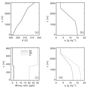
cu-Fig. 3. Initial profiles of: (a) potential temperature, (b) total water mixing ratio and (c) reactant mixing ratio (ppb) and (d) the initial profile of the total mixing ratio to simulate a clear boundary layer (dashed line) and a more cloudy boundary layer than the control simulation (dotted line). Notice the different vertical axis in panel (c).
mulus (Cuijpers and Duynkerke, 1993; Siebesma and Cui-jpers, 1995) and atmospheric turbulent reacting flows (Pe-tersen et al., 1999; Vil`a-Guerau de Arellano and Cuijpers, 2000).
The NCAR LES code has been described in Moeng (1984), Moeng (1986) and Sullivan et al. (1996). The code has recently been modified to run on massively parallel ma-chines using the Message Passing Interface (MPI) and is described in Patton et al. (2005). The NCAR code uses a pseudospectral and a second-order finite difference method for horizontal and vertical advection, respectively. Vertical scalar advection is performed using a limited κ=1/3 scheme (Koren, 1993). Time integration proceeds using a third-order Runge-Kutta method (Spalart et al., 1991). An Euler back-ward iteration method (Barth et al., 2003) is used to solve the chemistry. Similar to the WUR LES, subgrid-scale terms are parameterized with subgrid-scale turbulent kinetic en-ergy and stability dependent length scale. The condensation scheme is also based on the all-or-nothing assumption.
The initial conditions and surface forcing are the same as those prescribed by Brown et al. (2002). Figure 3 shows the initial profiles (05:30 LT) of the potential temperature, spe-cific humidity, and the reactants. Following the suggestion of Brown et al. (2002), the initial potential temperature profile has been slightly modified (see Fig. 10 in their paper) to sim-ulate a cloud top height that rises faster than their standard
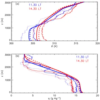
Fig. 4. Time evolution at 11:30 LT (17:30 UTC) and 14:30 LT (20:30 UTC) of vertical profiles of (a) potential temperature and (b) total-water mixing ratio. The thick solid lines show the one-hour averaged profiles obtained by the WUR-LES, the thick dashed lines show the one-hour averaged profiles obtained by the NCAR-LES. The thin solid lines are the observations taken by the radiosonde profile at the Southern Great Plains ARM C1 site and the thin dotted lines represent the values of the radiosounding launched at the site B5.
case. The surface fluxes of moisture and potential temper-ature vary with time following the measurements presented in Fig. 2. The only other external forcing is a prescribed westerly geostrophic wind equal to 10 m s−1. Small exter-nal tendencies representing the advection of heat and mois-ture are not included. Initial profiles of specific humidity for two sensitivity simulations are shown in Fig. 3d. The model domain size is 6400 m×6400 m×4400 m with a horizontal grid length equal to 66.7 m and a vertical grid length equal to 40 m. The simulations are integrated from 05:30 LT to 18:30 LT.
The chemical system is based on the atmospheric cycle of nitrogen dioxide, nitric oxide, and ozone. By using a simple chemical system, the influence of shallow cumulus on the transport of the species and on the photodissociation rates below, in and above the clouds can be clearly determined. The LES codes include the following two reactions:
NO2 j → NO + O3 (1) NO + O3 k → NO2, (2)
where j and k are first- and second-order chemical reaction rates, respectively. The initial mixing ratio profiles of NO2,
NO and O3 are shown in Fig. 3c. We also simulate an
in-ert tracer whose initial profile is zero. The surface fluxes are constant with time using the following values: inert tracer (0.1 ppb m s−1), NO
2(0.1 ppb m s−1), NO (0.05 ppb m s−1)
and O3 (0.0 ppb m s−1). The magnitude of the NO2 and
NO fluxes are fairly large in order to quickly obtain chemi-cal equilibrium in the production and destruction of the three species, i.e. 8=(k NO O3/j NO2)=1. By varying the
val-ues of j and k, one can study how the control of turbu-lence and the departure of chemical equilibrium influences the reactivity of the system. In the control simulation we use
j =8.3×10⁻³(s−1) and k=4.75×10⁻⁴(ppb s−1).
An important aspect of this study is to investigate the mod-ification of the photolysis rates by the presence of clouds. Because clouds alter the different proportions of direct and diffuse ultraviolet radiation, the actinic flux (and therefore the photolysis rates) has different values below, in, and above the clouds (Madronich, 1987). We have implemented this effect by calculating at every time step a factor below and above the clouds and by applying this factor to the clear sky value of the photolysis rate jclearfollowing Chang et al.
(1987):
jclouds=F jclear (3)
Above the cloud, the factor (F ) is defined as:
F =1 + α (1 − tr)cos(χo). (4)
While, below the cloud, F is defined as:
F =1.6 tr cos(χo). (5)
Here, tr is the energy transmission coefficient for normally incident light, χo is the solar zenith angle, and α is a reac-tion dependent coefficient (for nitrogen dioxide α=1.2). To simplify the calculation, a linear interpolation is assumed in-side the cloud. Based on measurements of jNO2(Fr¨uh et al.,
2000), the linear interpolation assumption likely overesti-mates the photolysis rate in the middle to lower regions of the cloud while underestimates the photolysis rate near cloud top.
The energy transmission coefficient tr depends on the cloud optical depth and a scattering phase function asym-metry factor (f ) equal to 0.86 for the typical cloud particle size ranges under study (Joseph et al., 1976). The expression reads:
tr =
5 − e−τ
[4 + 3τ (1 − f )]. (6)
The cloud optical depth (τ ) is calculated according to the expression given by Stephens (1984)
τ = 3
2
W ρl
re−1, (7)
where W is the vertically integrated liquid water (kg m−2),
ρl is the water density (kg m−3) and re is the effective ra-dius. Here, we have used a constant value of re=10 µm. For
J. Vil`a-Guerau de Arellano et al.: Transport and transformation in shallow cumulus 3223
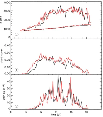
Fig. 5. Time evolution of: (a) cloud top height and cloud base height; of (b) cloud cover and of (c) liquid water path. Black: WUR-LES, Red: NCAR-LES.
clouds characterized by values of τ <5 and for regions be-tween clouds, we have assumed the photolysis rate of clear sky conditions. Regions between clouds may actually have enhanced photolysis rates due to cloud scattering. Here, we are simply investigating the importance of cloud scattering in the cloud column. Our control simulation includes the mod-ification of photolysis rates due to cloud scattering, while a sensitivity simulation excludes this effect on the chemistry.
2.3 Model validation: dynamics
The simulated and observed profiles of the potential tempera-ture and the total water specific humidity are shown in Fig. 4. Differences between observations and LES results are due to two reasons: (a) the LES simulations are based on an ide-alization of the initial conditions and of the surface bound-ary conditions, and (b) one-hour averaged LES results are compared with instantaneous soundings. Note that the aim of the validation with measurements is not to compare the exact values (as shown in Fig. 4 the vertical profiles of the radiosoundings at the site C1 and B also have large differ-ences), but to evaluate the ability of the LES to reproduce the dynamics of a shallow cumulus convection situation and to capture the observed vertical profile evolution.
The evolution of the vertical profiles of the state variables is as follows. At 11:30 LT, at the onset of clouds, obser-vations and LES results show three-distinct layers. In the
Fig. 6. Time evolution of the vertical profiles one-hour slab aver-aged (a) mixing ratio inert scalar, (b) mixing ratio NO2, (c) mixing
ratio NO and (d) mixing ratio O3. Solid line: WUR-LES, Dashed
line: NCAR-LES.
sub-cloud layer (up to 1000 m), there is a well-mixed layer in both observations and LES results. Above this layer, the cloud layer is still not conditionally unstable. Above cloud top (at around 1300 m) there is an absolutely stable boundary layer. This three layer structure is maintained at 14:30 LT. At this stage the clouds have matured. However, the cloud layer has deepened to ∼3000 m and is conditionally unstable. The two LES codes predict similar boundary layer evolution. The other cloud parameters (cloud cover, cloud base and cloud top heights, and liquid water path; Fig. 5) evolve similarly to those reported by Brown et al. (2002) (see their Fig. 5b), but because we prescribe a weaker liquid water potential temper-ature inversion, our results exhibit enhanced cloud vertical development. We find very good agreement of these cloud properties calculated by both LES codes. In concluding, in view of the evolution of the vertical profiles of the state vari-ables and their fluxes (not shown), we are confident of the ability of both LES codes to reproduce a daily evolution of shallow cumulus over land.
2.4 Model validation: chemistry
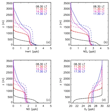
The evolution and the distribution of the reactants in this cloudy boundary layer are assessed by analyzing the mean vertical profiles, the fluxes, and the variances. Figure 6 shows the time evolution of the mean profiles of the inert scalar and the three reactants. The agreement between the results of both LES is very good. Both models show the growth of
Fig. 7. Time evolution of the one-hour slab averaged vertical pro-files of the resolved flux of: (a) mixing ratio inert scalar, (b) mixing ratio NO2, (c) mixing ratio NO and (d) mixing ratio O3. Solid line:
WUR-LES, Dashed line: NCAR-LES.
the boundary layer during the day and the enhancement of the transport in the cloud. Slight differences are found in the vertical profiles near the cloud top once the clouds are mature (see the profiles at 20:30 and 23:30). The NCAR-LES sim-ulates larger vertical transport between the sub-cloud layer and the cloud layer compared to WUR-LES due to a slightly larger buoyancy flux within the sub-cloud layer.
The evolution of the vertical flux profile of the species is demonstrated in Fig. 7. At 08:30 LT, both model results show the importance of the entrainment flux of reactants in the ini-tial period of the clear convective boundary layer growth. At 14:30 and 17:30 LT, larger fluxes occur inside the cloud layer due to the buoyant updraft motions driven by the release of latent heat. The flux enhancement of the species is also re-lated to the vertical variation of the photodissociation rates perturbed by the clouds (Eq. 3). Both model results show the enhancement of the flux of NO at 14:30 LT, with a max-imum value around z=1600 m. As shown in Fig. 3, NO has the lowest mixing ratio compared to NO2and O3. Thus, the
modification of the photolysis rate in the cloud will have a strong influence on the vertical distribution of species NO. Since the clouds are mature at 14:30 LT, the difference in the photolysis rate both in and below the cloud are larger. Larger gradients are created due to the different values of the first-order reaction rate, yielding to the increase of the flux.
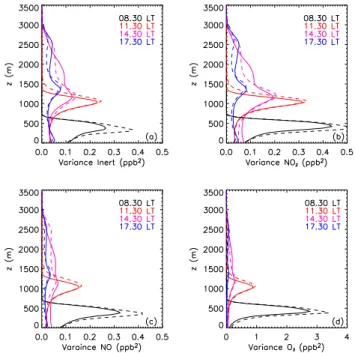
Satisfactory agreement between both LES models is also found for the evolution of the vertical profiles of the ances (Fig. 8). Before cloud formation (08:30 LT), the
vari-Fig. 8. Time evolution of vertical profiles of the one-hour slab aver-aged resolved variances of (a) mixing ratio inert scalar, (b) mixing ratio NO2, (c) mixing ratio NO and (d) mixing ratio O3. Solid line: WUR-LES, Dashed line: NCAR-LES.
ances between the models differ significantly in the entrain-ment zone as a result of the different subgrid-scale models used in each LES code. The NCAR and WUR-LES re-sults show that the largest concentration fluctuations occur at the interface between the sub-cloud and cloud layer. Be-cause of the cloud-induced updrafts, the scalar variance be-comes more vertically distributed within the cloud layer as the clouds reach maximum development (around 14:30 LT). In Sect. 4, we will discuss how the turbulence driven by the release of latent heat affects the mixing of reactants and their chemical reactivity.
3 Enhancement of the vertical transport
Large uncertainties in atmospheric chemistry models are as-sociated with the crude representation of boundary layer clouds in regional and large scale models (Dabberdt et al., 2004). In this section, we study the potential effects of cloud-induced changes on boundary layer structure, and con-sequently on the reactant concentrations, and evaluate a pre-liminary representation of the vertical transport in the clouds. Fair weather cumuli strongly modify the boundary layer structure by deepening its height, which in turn transports the sub-cloud compounds to the cloud layer.
In order to investigate the impact of clouds, we conduct an LES experiment where shallow cumulus clouds do not form (i.e. clear sky conditions). In this experiment, we pre-scribe the same initial and boundary conditions as in the
J. Vil`a-Guerau de Arellano et al.: Transport and transformation in shallow cumulus 3225
Fig. 9. Time evolution of the: (a) inert tracer height with clouds (black), inert tracer height without clouds (red), cloud top height (solid blue line) and cloud base height (blue dashed line), (b) the volume-averaged inert scalar mixing ratio for the cloudy case (CL, solid black) and the clear sky case (CS, red).
control simulation (see Sect. 2.2) except that we reduce the initial profile of the total water mixing ratio by 3 g kg−1(see Fig. 3d). In order to have an independent criterion to es-timate the maximum vertical transport of the reactants, we define a height (h) as a function of the mixing ratio of an inert tracer. h is defined as the height where the averaged mixing ratio becomes 0.5% of the horizontally-averaged mixing ratio in the sub-cloud layer. This height indicates maximum elevation where the scalar and reactants are vertically transported.
The evolution of h in the cloudy control simulation (CL) and the clear sky boundary layer (CS) is shown in Fig. 9a. In the cloudy boundary layer, h closely follows the cloud top height, which is defined as the highest elevation where liquid water is found in the entire domain, although at early times (e.g., 11:00 LT), h falls below the cloud-top height because only a limited number of clouds has formed. At later times (e.g., 17:00 LT) h persists at the highest elevation attained by the clouds during the day even though the clouds have de-cayed. The shallow cumulus clouds act to transport scalars to elevated regions in the cloud layer that remain there follow-ing the clouds’ dissipation. Consequently, the presence of clouds has an impact on the mixing ratio in the early stages of the formation of the nocturnal residual layer. In general, and depending on the strength of the thermal inversion above the cloud top, the reactants remain in the boundary layer and they are not transported to regions above the cloud layer in agreement with Cotton et al. (1995).
Fig. 10. Time evolution of the vertical profiles one-hour slab aver-aged (a) mixing ratio inert scalar, (b) mixing ratio NO2, (c) mixing
ratio NO and (d) mixing ratio O3. These profiles come solely from
the WUR-LES. Solid line: CL. Dashed line: CS.
The difference in h between the CS and CL simulations reaches its maximum at around 14:00 LT and the difference is approximately 600 m (Fig. 9a). The development of clouds has increased the depth over which species are transported and has direct impact on their evolution. To illustrate this, we calculate the volume averaged inert scalar mixing ratio for the CS and CL cases (Fig. 9b), which we call Acsand Acl, respectively. To calculate this volume average, we include all points in the horizontal domain from the ground surface up to each case’s respective h. Due to the larger volume in the cloudy case, Acldecreases at the onset of cloud development. When Cu are fully developed (after 14:00 LT), the difference between Acsand Acl can reach 50%.
Compared to the clear sky situation, clouds redistribute scalar species vertically (Fig. 10). Similar vertical profiles of carbon monoxide were shown by (Angevine, 2005) which in-dicate the enhanced vertical transport of species due to shal-low cumulus. In Fig. 10, before the onset of the clouds, the
CLand CS scalar profiles are similar. Following cloud de-velopment, the compounds are mixed through a larger ver-tical depth such that sub-cloud mixing ratios are reduced in the cloudy boundary layer. For instance, for NO2in the CL
case, the mixing ratio is reduced in the sub-cloud layer (at 500 m) by a factor 0.5%, 7% and 12% at, respectively, 11:30, 14:30, 17:30 LT compared to those in CS. Clouds tend to enhance the volume of the cloud layer through which species are transported and consequently dilute the concentration of boundary layer compounds. The redistribution of species to
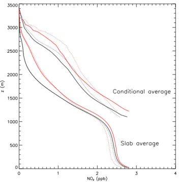
Fig. 11. One-hour averaged vertical profiles at 14:30 LT of the mix-ing ratio of the mixmix-ing ratio of NO2(horizontally-averaged over the
whole simulation domain) and of the mixing ratio of NO2
(condi-tionally average by calculating the average fields over grid points with a nonzero liquid water content). Solid lines represent the NO2 calculated with the photolysis rate jcloudand the dotted lines
rep-resent the NO2calculated with the photolysis rate jclear. Black: WUR-LES. Red: NCAR-LES.
higher altitudes can have a direct impact on the initial mix-ing ratios durmix-ing the evenmix-ing transition when the nocturnal residual layer is formed. With higher concentrations in the residual layer, the transfer of the previous day’s boundary layer compounds to the free troposphere would be enhanced. Investigations need to be pursued to assess the importance of shallow cumulus clouds on this mechanism of moving boundary layer compounds to the free troposphere.
To emphasize the impact of vertical scalar transport by shallow cumulus, we now investigate conditionally-averaged fields. Here, we define within-cloud conditionally-averaged fields by spatially averaging the compounds over the grid points containing liquid water (liquid water content greater than zero). Figure 11 presents one-hour averaged within-cloud field along with the horizontally averaged field over the whole domain for NO2at 14:30 LT. Two simulations are
shown: (a) using photolysis rate perturbed by clouds and (b) using the photolysis rate under clear sky conditions. The comparison of these two simulations will be discussed later in Sect. 5. Note that the results of the two LES models agree very well. As expected, the results indicate that the updrafts associated with the buoyant cumulus clouds are the main transport mechanism.
To test current parameterizations of cumulus convection used in large models, we compare horizontally-averaged
ver-tical scalar fluxes from the LES results to those estimated by the mass-flux parameterization (Betts, 1973; Arakawa and Schubert, 1974; Cotton et al., 1995). Briefly, in mass-flux schemes, the ABL is represented by strong updrafts inside the clouds (c) surrounded by the environment downdrafts (e). In this approach, the average value of a generic scalar ψ is calculated for both updrafts and downdrafts. The average value of the entire layer is decomposed as follows:
ψ = aψc+(1 − a)ψe, (8) where a denotes the cloud cover. The flux (Fψ) of the scalar
ψcan be written according to:
Fψ = ρw0ψ0 ≈ M(ψc−ψ ), (9) where M is by definition the mass flux which reads:
M ≡ ρacwc. (10) Here, acand wcdenote the cloud cover and vertical velocity calculated by the previously described conditional averaging method, respectively. Expression (9) is an approximation of the total flux and takes into account only the organized turbu-lent transport in the cloud and the environment (see Siebesma and Cuijpers, 1995).
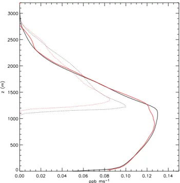
The results of the mass-flux approach for NO2are plotted
in Fig. 12. We found very consistent results in the compar-ison of the total flux and the mass-flux approximation cal-culated by the NCAR-LES and the WUR-LES. There is an underestimation by a factor 1.5 at cloud base whereas in the middle of the cloud the mass-flux approach represents the scalar flux quite well. Near cloud top, the mass-flux approach overestimates by a factor 1.5 compared to the LES-calculated total flux. These results are consistent with the previous study carried out by Siebesma and Cuijpers (1995) where they evaluate the mass-flux scheme for heat and total wa-ter. A key aspect that still requires further research is the ex-change flux between the sub-cloud layer and the cloud layer. As shown in Fig. 12 this flux is underestimated by the mass-flux approximation. For chemically reactive species, the ex-change flux is also modified by the cloud-imposed photoly-sis rate dependence (see the flux profile at Fig. 7c). Greenhut (1986) quantified the transport of ozone by cumulus clouds from aircraft observations. They found that cloud turbulence accounts for ∼30% of the total cloud flux, whereas our LES results show that the organized turbulence in the clouds con-tributes more than 50% of the total cloud flux.
We also examine the species transport rate per unit time by integrating the flux divergence term included in the reactants’ conservation equation over height. The integral reads:
1 zct −zcb Z zct zcb ∂w0c0 i ∂z dz, (11)
where zcband zctdenote the cloud base and cloud top height, respectively, and w0c0
J. Vil`a-Guerau de Arellano et al.: Transport and transformation in shallow cumulus 3227
by the model. The horizontally-averaged vertical flux diver-gence integrated from cloud base to cloud top quantifies the net transport of species from the sub-cloud layer to the cloud layer. For NO2in the control case, we obtain values ranging
from 1 ppb hr−1at cloud onset to 0.2 ppb hr−1once the cloud has fully developed. We also calculate this rate in a simula-tion with higher cloud fracsimula-tion, which had maximum values
>0.5 between 14:00 and 16:00 LT, compared to the values around 0.2 of the control simulation. This simulation was done by increasing the initial total specific humidity profile as shown by the dotted line in Fig. 3d. Despite higher cloud fraction, the flux divergence of NO2was approximately the
same as was found in the control simulation. This small de-pendence on the cloud cover indicates that shallow cumulus are more vigorous and just as effective at transporting species when the sky is not completely cloud covered compared to when clouds cover most of the sky. Vukovich and Ching (1990) estimated similar rates of species transport, but their calculations revealed greater cloud cover dependency.
Currently, for state variables like the liquid water poten-tial temperature and the total water mixing ratio, the ex-change flux is parameterized by combining a turbulent clo-sure scheme in the sub-cloud layer (i.e., a function of an ex-change coefficient and the gradient of the variable) with the mass-flux closure in the cloud layer. As discussed thoroughly by Lenderink et al. (2005), there are still large uncertain-ties and discrepancies in the representation of these fluxes in large scale models. Based on our LES results, we con-clude that schemes which describe shallow cumulus should first accurately estimate the evolution of the boundary layer depth and second describe the enhanced vertical transport of reactants. Besides, the increase of dilution in the sub-cloud layer and the vertical transport in the cloud layer can have an impact on the atmospheric chemistry occurring in the stable and the residual layers once the convective boundary layer has collapsed.
4 Control of the reactivity by turbulent mixing
Organized turbulence can segregate reactants by transporting them in opposite directions (see for instance the initial pro-files of NO and O3 in Fig. 3) and can therefore limit their
chemical reactivity: reactants must be mixed before the reac-tion takes place. In particular, turbulent control of reactivity becomes important if the turbulent mixing time scale (τt) is similar to the time scale of chemical reaction (τc), i.e. when the Damk¨ohler number (Da=τt/τc) is O(1). The turbulent time scale is calculated by the expression w∗/zi, where w∗ is the characteristic convective velocity scale and zi is the boundary layer height. In our calculations, w∗is determined following Frisch et al. (1995) and zi is found by the local gradient method (Sullivan et al., 1998), which determines the local inversion height based on the maximum of the liq-uid water potential temperature gradient. The time scale of
Fig. 12. One-hour average vertical profiles of the total flux of NO2
(solid line) (horizontally-averaged over the whole simulation do-main) and of the parameterized mass flux of NO2 (dotted line). Black: WUR-LES. Red: NCAR-LES.
chemistry is calculated as (j )−1for a first-order reaction and as (kC)−1for a second-order reaction, where C is the mixing ratio of the reactant.
In dry convective boundary layers (Schumann, 1989; Molemaker and Vil`a-Guerau de Arellano, 1998), this control is quantified by defining the intensity of segregation I s which is the ratio of the covariance between reactants normalized by the ensemble horizontal mixing ratio average. This di-mensionless variable reads:
I s = ci0c0j ci cj
. (12)
For second-order chemical reactions, the covariance be-tween reactants appears explicitly in their governing equa-tion. Therefore, I s can be a measure the concentration fluc-tuation correlation’s importance in determining their ensem-ble means.
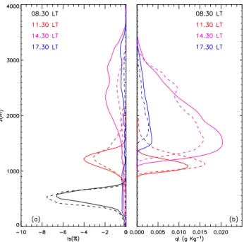
In Fig. 13, we show vertical profiles of I s between NO and O3and the liquid water content. The results of both LESs
show the close relation between the vertical cloud develop-ment and the I s-evolution. Two distinct turbulent layers are found under the presence of Cu (see for instance Fig. 6c in Brown et al., 2002). In the sub-cloud layer, even though the variances of reactive species are large (Fig. 8), the covariance (or I s) between NO and O3is almost negligible. This implies
that the reactants NO and O3are well mixed before reaction
Fig. 13. Time evolution of the vertical profile (one-hour slab aver-aged) of the (a) intensity of segregation of NO and O3and of the (b) liquid water content. WUR-LES: solid line and NCAR-LES dashed line.
layer where species transported in opposite directions could remain segregated.
The maximum values of I s range from 5% at the early stages of the cloud formation (11:30 LT) to 3% when clouds are mature (14:30 LT). The absolute values of these I s-profiles are rather low compared to ones in the previous stud-ies concerning dry convective boundary layers. Because w∗ and zi change during the simulations, the turbulent timescale and therefore the Damk¨ohler number have a range of values,
τt=10–40 min and Da=4–20. Thus, our chemical system is characterized by a Da>1, which indicates that the chemistry is much faster than the turbulent mixing. One may expect higher absolute values of I s in more complex chemical sys-tems where Damk¨ohler numbers of some reactions are O(1) and in situations where the chemistry departs from the pho-tochemical equilibrium state.
5 Perturbation of the photolysis rate by the clouds
To study the effect of clouds on the photolysis rate, we carry out two simulations using the two LES codes. The first one, the control simulation discussed in the previous sec-tions, takes into account the perturbation of the j -values by clouds using Expression (3) (jcloudy). The second
simula-tion assumes a constant photolysis rate with height and time and therefore the photodissociation rates are not perturbed by the Cu (jclear). Our aim is to: 1) analyze the modification
of the reactant distribution resulting from the cloud
radia-Fig. 14. Instantaneous vertical cross section at 14:30 LT of the liquid water mixing ratio (blue shading) and the % difference of the mixing ratio of NO2calculated with the photolysis rate jcloudy
(NO2cl) minus the mixing ratio of NO2calculated using the
pho-tolysis rate jclear(NO2cs). The red lines show positive differences
(mixing ratio calculated with jcloudyis higher than the one calcu-lated with jclear). The black lines show negative differences.
Pan-els: (a) Damk¨ohler number range of 0.4–2.0, (b) Damk¨ohler num-ber range of 4–20, and (c) Damk¨ohler numnum-ber range of 40–200.
tion perturbation, and 2) investigate the dependence of this modification to temporal and spatial averaging. In Fig. 14, we show the following variables: 1) an instantaneous cross section of the liquid water content, and 2) the mixing ratio difference of NO2 calculated using jcloudy minus that
cal-culated using jclear. The vertical cross section corresponds
to the time when the shallow cumulus were fully developed (around 14:30 LT). In the figure, we have also included the sensitivity of the results to the Damk¨ohler number by repeat-ing the same simulation usrepeat-ing the same initial and boundary conditions, but changing the chemical reaction rate. The fol-lowing first- and second-reaction rates are prescribed:
Figure Da j(s−1) k(ppb s)−1
14a 0.4–2.0 8.3×10⁻⁴ 4.75×10⁻⁵
14b (Control) 4.0–20. 8.3×10⁻³ 4.75×10⁻⁴
14c 40.–200. 8.3×10⁻² 4.75×10⁻³
In Fig. 14, the three cases reveal similar spatial patterns with regards to the cloud effect on the photodissociation rates. In the lower portion of the cloud and in the sub-cloud
J. Vil`a-Guerau de Arellano et al.: Transport and transformation in shallow cumulus 3229
layer, we find larger values of the mixing ratio calculated by using jcloudy. In this region where jcloudy<jclear, clouds
de-crease the reactivity resulting in NO2cl>NO2cs. In the upper part of the cloud, the opposite effect is found; due to the en-hancement of the actinic flux (jcloudy>jclear) NO2cl<NO2cs.
As shown, the order of magnitude of this effect is a func-tion of the Damk¨ohler number. The case where Da=0.4– 2.0 (Fig. 14a), shows differences of about ±10% at cloud top and cloud base compared to the case using a constant
j-value. When Da=40–200, this difference increases con-siderably (Figs. 14b and 14c): 40% in the sub-cloud layer and −20% in the upper cloud region. This sensitivity reveals a coupling between chemistry driven by ultraviolet radiation and the turbulent transport under the presence of the clouds. Due to these differences, we find that the presence of clouds induce deviations from the photostationary state equilibrium
8=kNO O3/j NO2=1. In the control simulation, 8 ranges
from 0.8 in the cloud to 1.4 below clouds. The calculation is based on the instantaneous mixing ratio values.
In reactive turbulent flows characterized by Da<1, the tur-bulent transport time scale is faster than the chemical reac-tivity scale, implying that turbulence can efficiently transport and mix the species before chemical reactions occur. As a re-sult, the mixing ratio gradients tend to decrease by turbulent mixing. However, in flows with Da>1, because the chemical reactivity is faster than the mixing, the reactivity maintains scalar gradients which increase the effect of the perturbed photolysis rates. It is important to note that the Damk¨ohler number can vary spatially in cloudy boundary layers. Be-cause the buoyant convection enhances vertical velocities in the cloud cores, the convective velocity scale becomes spa-tially heterogeneous inducing a large variability in Da. As a consequence, effects of the modified photolysis rates can be-come larger in certain regions depending on the local value of Da.
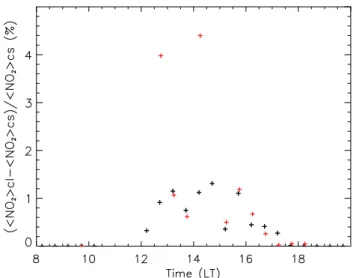
By doing temporal and spatial averaging, we can further study the impact of different photolysis rates (jcloudy and jclear) on the reactant distribution. In Fig. 15, we plot the
dif-ferences of the mixing ratio for NO2calculated using jcloudy
(NO2cl) and jclear (NO2cs) from the surface to cloud top
(30-min average). Except for the two peaks at around 13:00 and 14:00 LT calculated by NCAR-LES results, the two LES codes give variations of around 2%. This value contrasts with the larger values of ∼40% reported in Fig. 14. Thus, the pho-tolysis rate disturbed by clouds has a large impact on the in-stantaneous mixing ratios locally, but its impact is smoothed by averaging in time and space. Since our chemical system is close to an equilibrium, the impact of local variations be-comes minimal by averaging.
To complete this study, we calculate the conditionally av-eraged mixing ratios computed using jcloudyand jclear
(pre-sented in Fig. 11). The one-hour average vertical profiles show different values for the profiles NO2cland NO2cs. The
results from the two LESs show very similar structure: large depletion of NO2 near cloud base by the simulation using
Fig. 15. Time evolution of the percent difference of the volume averaged mixing ratio of NO2from surface to cloud top (cross)
cal-culated with the photolysis rate jcloud (NO2cl) minus calculated
using the photolysis rate jclear (NO2cs) Black: WUR-LES. Red:
NCAR-LES.
jclear and larger depletion of NO2in the upper cloud region
by the simulation using jcloud. The differences are higher
than the ones shown in Fig. 15. Near cloud base, they range from 4% to 12% and near cloud top (around 2500 m) are
−15%.
In view of the different results shown in Figs. 11, 14 and 15, it is very difficult to provide a conclusive state-ment as to the effect of modified photodissociation in clouds on the reactant distribution. Locally and at short time scales, the perturbation can modify the chemistry by enhanc-ing/diminishing the concentration fields and by perturbing the establishment of possible chemical equilibrium. How-ever, this perturbation by clouds can be smoothed out by time and space averaging. It is important to mention that these large fluctuations of the reactant fields can also be relevant in analyzing field measurements in and around shallow cu-mulus. By temporally and spatially averaging, the induced variability generated by the presence of clouds is filtered out which could lead to errors interpreting measurements.
6 Conclusions
The effects of shallow cumulus dynamics and radiation on three chemical species are studied by analyzing and com-paring results from two large-eddy simulation codes: NCAR and WUR. The chemical system is composed by a first- and second-order reaction near a chemical equilibrium. Both LES codes satisfactorily reproduce the diurnal evolution of shallow cumulus over land based on a situation observed on 21 June 1997. With respect to the diagnostic fields of the
three reactants, we find very good agreement in the evolution of the mean, fluxes, and (co-)variances.
The presence of clouds increases the volume in which species are transported, which leads to a dilution of reactant mixing ratio within the boundary layer. Mixing ratios of trac-ers below cloud decrease by up to 12% while mixing ratios averaged in the volume defined from the surface to the max-imum elevation where tracers are vertically transported de-crease by up to 50% compared to the clear sky situation. Fur-thermore, reactants transported to elevated regions remain at those levels following the clouds’ dissipation, which should have an effect on simulating nocturnal chemistry of the resid-ual layer.
Analysis of the enhancement of the vertical transport re-veals that the buoyant upward motions are responsible for transporting the reactants in the cloud. Current parameteri-zations based on the mass-flux approach adequately describe the transport in mid-cloud, but they tend to underestimate the flux at cloud base by a factor 1.5, showing the need to improve the parameterization of reactant exchange between the sub-cloud and cloud layers. The variability of the species quantified by the mixing ratio variance profile is closely as-sociated with the cloud development and is characterized by two maxima, one in the sub-cloud layer and the other within the cloud layer. Our analysis also shows that species are uni-formly mixed in the sub-cloud layer, but that in the cloud layer reactants transported in opposite direction are some-what segregated and therefore the turbulence might control their reactivity. The control is expected to be larger when the time scale of turbulence is similar to the time scale of chemistry, namely when the Damk¨ohler number is O(1). We found that the reaction rate is reduced between 2% and 5% at different stages of the cloud development. We note that these absolute values can increase if the reactants depart from pho-tochemical equilibrium.
The perturbation of photodissociation rates due to the pres-ence of clouds is discussed comparing a simulation that uses a photodissociation rate perturbed by the cloud with one that uses clear sky values. By analyzing the instantaneous fields of the mixing ratio, we find differences up to 40% below the cloud base height and up to 20% close to cloud top, which in-dicates a large variability in the reactant distribution, an im-portant aspect in the interpretation of the chemical processes in and around clouds. These differences are dependent on the capacity of the vertical transport to smooth out the gra-dients created by the perturbed photodissociation rates, i.e. depending on the Damk¨ohler number. For turbulent reacting flows characterized by values Da∼O(1) and larger, we find that turbulence decreases mixing ratio gradients created by the different photodissociation rates below, in and above the cloud. These differences are significantly reduced to values of ∼1% when averaged over the cloudy boundary layer in both space and time. Further studies will attempt to investi-gate and to complete these findings in more complex chem-ical mechanisms, to explore the effect of cloud penetration
into the free troposphere on the distribution of reactants and the influence of shallow cumulus on the initial formation of the nocturnal residual layer.
Acknowledgements. J. Vil`a was partially supported for his visit at
NCAR by the Netherlands Organization for Scientific Research NWO (project 76/241). The WUR-LES numerical simulations were financially supported by NCF (SG-132). We appreciate the fruitful discussions with C.-H. Moeng. We thank D. Lenschow and T. Karl for their comments on the work. The National Center for Atmospheric Research is operated by the University Corporation for Atmospheric Research under the sponsorship of the National Science Foundation.
Edited by: S. Galmarini
References
Angevine, W. M.: An integrated turbulence scheme for boundary layers with shallow cumulus applied to pollutant transport, J. Appl. Meteorol., 44, 1436–1452, 2005.
Arakawa, A. and Schubert, W. H.: Interaction of a cumulus cloud ensemble with the large scale environment, J. Atmos. Sci., 31, 674–701, 1974.
Barth, M. C., Sillman, S., Hudman, R., Jacobson, M. Z., Kim, C.-H., Monod, A., and Liang, J.: Summary of the cloud chemistry modeling intercomparison: Photochemical box model simula-tion, J. Geophys. Res., 108, 4214, doi:10.1029/2002JD002673, 2003.
Baumann, K., Willimas, E. J., Angevine, W. M., Roberts, J. M., Norton, R. B., Frost, G. J., Fehsenfeld, F. C., Springston, S. R., Bertman, S. B., and Hartsell, B.: Ozone production and trans-port in Nashville, Tennessee: results from the 1994 study at New Hendersonville, J. Geophys. Res., 105, 9137–9153, 2000. Betts, A. K.: Non precipitating cumulus convection and its
param-eterization, Quart. J. Roy. Meteorol. Soc., 99, 178–196, 1973. Brown, A. R., Cederwall, R. T., Chlond, A., Duynkerke, P. G.,
Go-laz, J., Khairoutdinov, J. M., Lewellen, D., Lock, A., Macveen, M. K., Moeng, C., Neggers, R. A. J., Siebesma, A. P., and Stevens, B.: Large-eddy simulation of the diurnal cycle of shal-low cumulus convection over land, Quart. J. Roy. Meteorol. Soc., 128(B), 1075–1094, 2002.
Chang, J., Brost, R., Isaksen, I., Madronich, S., Middleton, P., Stockwell, W., and Walcek, C. J.: A three-dimensional Eule-rian acid deposition model: physical concepts and formulation, J. Geophys. Res., 92, 14 681–14 700, 1987.
Ching, J. K. S. and Alkezweeny, A. J.: Trace study of vertical ex-change by cumulus clouds, J. Clim. Appl. Meteorol., 25, 1702– 1711, 1986.
Ching, J. K. S., Shipley, S. T., and Browell, E. V.: Evidence for cloud venting of mixed layer ozone and aerosols, Atmos. Envi-ron., 22, 225–242, 1988.
Cotton, W. R., Alexander, G., Hertenstein, R., Walko, R., McAnelly, R., and Nicholls, M.: Cloud venting – a review and some new global annual estimates, Earth Sci. Rev., 39, 169–206, 1995.
Cuijpers, J. W. M. and Duynkerke, P. G.: Large eddy simulations of trade wind with cumulus clouds, J. Atmos. Sci., 50, 3894–3908, 1993.
J. Vil`a-Guerau de Arellano et al.: Transport and transformation in shallow cumulus 3231
Dabberdt, W. F., Carroll, M. A., Baumgardner, D., Carmichael, G., Cohen, R., Dye, T., Ellis, J., Grell, G., Grimmond, S., Hanna, S., Irwin, J., Lamb, B., Madronich, S., McQueen, J., Meagher, J., Odman, T., Pleim, J., Schmidt, H. P., and Westphal, D. L.: Me-teorological research needs for improved air quality forecasting, Bull. Amer. Meteorol. Soc., 85, 563–586, 2004.
Frisch, A. S., Lenschow, D. H., Fairall, C. W., Schubert, W. H., and Gibson, J. S.: Doppler radar measurements of turbulence in marine stratiform cloud during ASTEX, J. Atmos. Sci., 52, 2800–2808, 1995.
Fr¨uh, B., Trautmann, T., Wendisch, M., and Keil, A.: Comparison of observed and simulated NO2photodissociation frequencies in a cloudless atmosphere and in continental boundary layer clouds, J. Geophys. Res., 105, 9843–9857, 2000.
Greenhut, G.: Transport of ozone between boundary layer and cloud layer by cumulus clouds, J. Geophys. Res., 91, 8613–8622, 1986.
Joseph, J. H., Wiscombe, W. J., and Weinman, J. A.: The delta-Eddington approximation for radiative transfer flux, J. Atmos. Sci., 33, 2452–2458, 1976.
Koren, B.: A robust upwind discretization method for advection, diffusion and source terms, in: Notes on Numerical Fluid Me-chanics, edited by: Vrengdenhil, C. B. and Koren, B., Vieweg-Braunschweig, vol. 45, chap. 5, pp. 117–138, 1993.
Lenderink, G., Siebesma, A. P., Cheinet, S., Irons, S., Jones, C. G., Marquet, P., Muller, F., Olmeda, D., Calvo, J., Sanchez, E., and Soares, P. M. M.: The diurnal cycle of shallow cumulus over land: a single column model intercomparison study, Quart. J. Roy. Meteorol. Soc., 130, 3323–3328, 2004.
Lenderink, G., Siebesma, A. P., Cheinet, S., Irons, S., Jones, C. G., Marquet, P., M¨uller, F., Olmeda, D., Calvo, J., Sanchez, E., and Soares, P. M. M.: The diurnal cycle of shallow cumulus clouds over land: a single column model intercomparison study, Quart. J. Roy. Meteorol. Soc., 123, 223–242, 2005.
Madronich, S.: Photodissociation in the atmosphere: 1. Actinic fluxes and the effects of ground reflections and clouds, J. Geo-phys. Res., 92, 9740–9752, 1987.
Moeng, C.-H.: A large-eddy simulation model for the study of plan-etary boundary-layer turbulence, J. Atmos. Sci., 41, 2052–2062, 1984.
Moeng, C. H.: Large-eddy simulation of a stratus-topped boundary layer: Part I. Structure and budgets, J. Atmos. Sci., 43, 2886– 2900, 1986.
Molemaker, M. J. and Vil`a-Guerau de Arellano, J.: Turbulent con-trol of chemical reactions in the convective boundary layer, J. Atmos. Sci., 55, 568–579, 1998.
Patton, E. G., Sullivan, P. P., and Moeng, C.-H.: Influence of ide-alized heterogeneity on wet and dry planetary boundary layers coupled to the land surface, J. Atmos. Sci., 62, 2078–2097, 2005. Petersen, A. C., Beets, C., van Dop, H., Duynkerke, P. G., and Siebesma, A. P.: Mass-flux characteristics of reactive scalars in the convective boundary layer, J. Atmos. Sci., 56, 37–56, 1999. Piacsek, A. P. and Williams, G. P.: Conservative properties of
con-vection difference schemes, J. Comput. Phys., 6, 392–405, 1970. Schumann, U.: Large-eddy simulation of turbulent diffusion with chemical reactions in the convective boundary layer, Atmos. En-viron., 23, 1713–1729, 1989.
Siebesma, A. P. and Cuijpers, J. W. M.: Evaluation of parametric assumptions for shallow cumulus convection, J. Atmos. Sci., 52, 650–666, 1995.
Spalart, P. R., Moser, R. D., and Rogers, M. M.: Spectral methods for the Navier-Stokes equations with one infinite and two peri-odic directions, J. Comput. Phys., 97, 297–324, 1991.
Stephens, G.: The parameterization of radiation for numerical weather prediction and climate models, Mon. Wea. Rev., 112, 826–867, 1984.
Sullivan, P., Moeng, C. H., Stevens, B., Lenschow, D. H., and Mayor, S. D.: Structure of the entrainment zone capping the con-vective atmospheric boundary layer, J. Atmos. Sci., 55, 3042– 3064, 1998.
Sullivan, P. P., McWilliams, J. C., and Moeng, C.-H.: A grid nesting method for large-eddy simulation of planetary boundary-layer flows, Bound.-Layer Meteorol., 80, 167–202, 1996.
Verwer, J. G.: Gauss Seidel iterations for stiff ODEs from chemical kinetics, SIAM J. Sci. Comput., 15, 1243–1250, 1994.
Vil`a-Guerau de Arellano, J. and Cuijpers, J. W. M.: The chemistry of a dry cloud: the effects of radiation and turbulence, J. Atmos. Sci., 57, 1573–1584, 2000.
Vukovich, F. M. and Ching, J. K.: A semi-empirical approach to estimate vertical transport by nonprecipitating convective clouds on a regional scale, Atmos. Environ., 24, 2153–2168, 1990.