Ecole des JDMACS 2011- GT MOSAR Synth` ese de correcteurs : approche bas´ ee sur
la forme observateur/retour d’´ etat MATLAB Tutorial session
D. Alazard
Let us consider the simplified model of a launcher:
G
0(s) = Y (s)
U(s) = 1 s
2− 1 ,
and the following candidate controllers (positive feedback):
K
0(s) = −23s − 32
s + 12 , K
1(s) = − s
2+ 27s + 26
s
2+ 7s + 18 , K
2(s) = − 1667s + 2753 s
2+ 27s + 353 .
1 Observer-based realization
1.a) Give a state space realization of G
0(s) with state vector x = [y y] ˙
T, 1.b) Compute an observer-based realization of controller K
1(s) (macro-function
cor2obr or cor2obra and obr2cor).
1.c) Plot the closed-loop response of plant and controller states to initial conditions: y(t = 0) = 1; ˙ y(t = 0) = −1.
1.d) Same things (1.b) and 1.c)) with controller K
2(s).
2 Cross standard form
Let us consider K
0(s). K
0(s) was designed to assign the closed-loop dominant dynamics to −1 ± i.
2.a) Compute the matrix T
1×2of the linear combination of plant states observed by controller state: x
K= T x b (macro-function cor2tfg or cor2tfga),
1
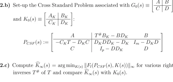
2.b) Set-up the Cross Standard Problem associated with G
0(s) ≡
"
A B C D
#
and K
0(s) ≡
"
A
KB
KC
KD
K#
:
P
CSF(s) :=
A T
#B
K− BD
KB
−C
KT − D
KC D
KDD
K− D
KI
m− D
KD
C I
p− DD
KD
2.c) Compute K c
∞(s) = arg min
K(s)kF
l(P
CSF(s), K(s))k
∞for various right inverses T
#of T and compare K c
∞(s) with K
0(s).
2.d) The frequency-domain response of the controller must now fit the fol- lowing template:
10−1 100 101 102 103
−40
−30
−20
−10 0 10 20 30 40
Singular Values
Frequency (rad/sec)
Singular Values (dB)
Figure 1: Frequency-domain responses (magnitude) of K
0(s) (solid line) and K c
∞(s) (dashed line) and template (grey patch).
Augment the standard problem P
CSF(s) to take into account this frequency- domain specification (Figure 2) and compute such a controller K c
∞(s).
Check the closed-loop dynamics.
2.e) Now, the actuator dynamics A(s) =
s+55≡
"
−5 5
1 0
#
is taken into account. Compute stability margins of the controller K c
∞(s) on the plant G
0(s)A(s).
2
u y w z
W (s) P CSF (s)
Figure 2: P
CSFwith frequency weight.
2.f ) Augment the previous standard problem with A(s) (Figure 3) and tune W (s) to find a controller K(s) fitting the template (Figure 1) and such c that the open loop transfer −G
0(s)A(s) K c (s) has at least a 30 deg phase margin.
u y
w z
W (s)
P
CSF(s) A(s)
Figure 3: P
CSFwith frequency weight and actuator dynamics.
2.g) Compute an observer-based realization of K(s) on the plant c G
0(s)A(s).
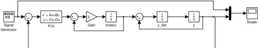
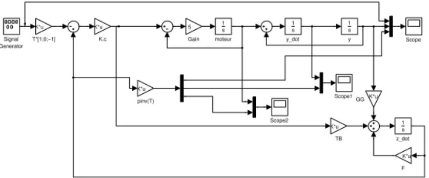
2.h) Plot responses to initial conditons ˙ y(t = 0) = −1 and to a square reference signal using the controller K c (s) directly (Figure 4) or using its observer based realization (Figure 5).
y_dot 1 s
y 1 s moteur
1 s Signal
Generator
Scope K(s)
x’ = Ax+Bu y = Cx+Du
Gain 5
Figure 4: Closed-loop simulation with controller K c (s).
3
z_dot 1 s y_dot
1 s
y 1 s
pinv(T) K*u
moteur 1 s
TB K*u T*[1;0;−1]
K*u Signal Generator
Scope2
Scope1
Scope K.c
K*u
Gain 5
GGK*u
F K*u