A Data-Driven Neuromuscular Model of Walking
and its Application to Prosthesis Control
by
Jared Markowitz
B.S., Carnegie Mellon University (2004)
Submitted to the Department of Physics
in partial fulfillment of the requirements for the degree of
Doctor of Philosophy
at the
MASSACHUSETTS INSTITUTE OF TECHNOLOGY
OF TECHNOLOGY
SEP
04 2013
LIBRARIES
June
2013
@
Massachusetts Institute of Technology 2013. All rights reserved.
f'i
Author ...
Certified by...
Department of Physics
May 24, 2013
...Hugh M. Herr
Associate Professor
Thesis Supervisor
C ertified by ...
Leonid A. Mirny
Associate Professor
Thesis SupervisorA ccepted by ...
...
John Belcher
Associate Department Head for Education
A Data-Driven Neuromuscular Model of Walking and its
Application to Prosthesis Control
by
Jared Markowitz
Submitted to the Department of Physics on May 24, 2013, in partial fulfillment of the
requirements for the degree of Doctor of Philosophy
Abstract
In this thesis we present a data-driven neuromuscular model of human walking and its application to prosthesis control. The model is novel in that it leverages tendon elasticity to more accurately predict the metabolic consumption of walking than con-ventional models. Paired with a reflex-based neural drive the model has been applied in the control of a robotic ankle-foot prosthesis, producing speed adaptive behavior.
Current neuromuscular models significantly overestimate the metabolic demands of walking. We believe this is because they do not adequately consider the role of elas-ticity; specifically the parameters that govern the force-length relations of tendons in these models are typically taken from published values determined from cadaver stud-ies. To investigate this issue we first collected kinematic, kinetic, electromyographic
(EMG), and metabolic data from five subjects walking at six different speeds. The
kinematic and kinetic data were used to estimate muscle lengths, muscle moment arms, and joint moments while the EMG data were used to estimate muscle activa-tions. For each subject we performed a kinematically clamped optimization, varying the parameters that govern the force-length curve of each tendon while simultaneously seeking to minimize metabolic cost and maximize agreement with the observed joint moments. We found a family of parameter sets that excel at both objectives, provid-ing agreement with both the collected kinetic and metabolic data. This identification allows us to accurately predict the metabolic cost of walking as well as the force and state of individual muscles, lending insight into the roles and control objectives of different muscles throughout the gait cycle.
This optimized muscle-tendon morphology was then applied with an optimized linear reflex architecture in the control of a powered ankle-foot prosthesis. Specifi-cally, the model was fed the robot's angle and state and used to command output torque. Clinical trials were conducted that demonstrated speed adaptive behavior; commanded net work was seen to increase with walking speed. This result supports both the efficacy of the modeling approach and its potential utility in controlling life-like prosthetic limbs.
Thesis Supervisor: Hugh M. Herr Title: Associate Professor
Thesis Supervisor: Leonid A. Mirny Title: Associate Professor
Acknowledgments
There are many people I need to thank for helping me complete my thesis work and navigate through my time at MIT. First I must thank Hugh for his guidance, for being a source of inspiration, and for his belief in me. I very much appreciate him giving me the chance to work in the Biomechatronics group and the generosity he has exhibited towards me over the years. I also appreciate the guidance given to me
by my thesis committee- Leonid Mirny, Mehran Kardar, and Jeff Gore. I thoroughly
enjoyed the classes they taught me here and greatly value both the thoughts they had about my project and the patience they displayed as I rushed to complete this work. I've also been quite fortunate to encounter several extremely helpful people from other institutions. I owe a huge debt of gratitude to Peter Loan, the author of the SIMM software. Peter has been an invaluable resource the last few years and without his help this thesis would not have been possible'. I'd like to thank Dan Lieberman for his generosity in letting me use his motion capture facility as well as Adam Daoud and Anna Warrener for helping me troubleshoot the system. I have also received extremely helpful advice about my work from Brian Umberger, Alena Grabowski, Cara Lewis, and Greg Sawicki. It is truly a privilege to work in a field with so many talented, helpful, and generally exceptional people.
One of the dominant factors in determining the quality of one's graduate career is the environment of their research group. I've been lucky enough to work in a group full of committed, gifted, and friendly people. We have all greatly benefited from the efforts of our administrator, Sarah Hunter, who is truly the glue that holds the group together. We have also all benefited from the excellent advice provided by Bruce Deffenbaugh, who always seems to turn up when most needed. I personally have been privileged to share an office with some of the best and brightest that MIT has to offer- Andy Marecki, David Sengeh (the future president of Sierra Leone), and Luke Mooney. I truly admire the work that they do and greatly appreciate them putting up with my idiosyncrasies. I also must thank Michael Eilenberg and Grant Elliott,
'Peter is so committed to helping SIMM users that he brought me a water bottle while I was running the 2011 Chicago Marathon. Pretty exceptional customer service.
who helped me get through some rough times in the lab and have generally been good and loyal friends. I would be remiss not to mention Ernesto Martinez-Villalpando, Ken Endo, David Hill, Madalyn Berns, Pavitra Krishnaswamy, Jiun-Yih Kuan, Reza Safai-naeeni, Elliott Rouse, Olli Kannape, Todd Farrell, and Arthur Petron- it has been a pleasure to work with all of you.
I must also thank my friends and family. I've been lucky enough to make many
great friends during my time in Cambridge through the lab, the Tech Catholic Com-munity, and through running. They have greatly brightened my time here and gen-erally made the experience worthwhile. Finally I would like to thank my family-parents Jared and Mary Helen and siblings Geoffrey, Anna, and Kathryn. It is hard to overstate how blessed I am to have them, and it is to them that I dedicate this thesis.
Contents
1 Introduction 19
1.1 Context . . . . 20
1.1.1 Inverse Modeling . . . . 20
1.1.2 Forward Modeling . . . . 21
1.1.3 Application to Prosthesis Control . . . . 21
1.2 Research Objectives. . . . . 22 1.3 Thesis Outline. . . . . 22 2 Background 25 2.1 Human Walking . . . . 25 2.1.1 Gait Cycle . . . . 25 2.1.2 Energetics . . . . 26
2.2 Muscles of the Leg . . . . 27
2.3 Muscle Physiology . . . . 29
2.3.1 Structure . . . . 29
2.3.2 Contraction Dynamics . . . . 30
2.3.3 Muscle Force Generation Models . . . . 31
2.4 Tendon Physiology . . . . 32
2.5 Neural-Structural Interactions . . . . 33
2.6 Neural Control and the Role of Reflexes . . . . 34
3 Muscle-Tendon Morphology Optimization
3.1 Methods .... ...
3.1.1 Data Collection ...
3.1.2 Data Processing Procedures . . . .
3.1.3 Muscle Activation Estimation . . . . 3.1.4 Muscle-Tendon System Identification . . . . .
3.2 R esults . . . .
3.2.1 Choosing an Optimal Solution . . . .
3.2.2 Metabolic Cost Predictions . . . .
3.2.3 Resolving Redundancy in Joint Actuation . . 3.2.4 Evaluating Muscle State . . . .
3.3 D iscussion . . . .
4 Pilot Application to Powered Ankle-Foot Prosthesis 4.1 Background . . . . 4.2 M ethods . . . . 4.2.1 M odeling . . . . 4.2.2 Application to Prosthesis Control . . . . 4.2.3 Powered Ankle-Foot Prosthesis . . . . 4.2.4 Knee Clutch . . . . 4.2.5 Angle Measurements . . . . 4.2.6 Electronics . . . . 4.2.7 Control . . . . 4.2.8 Torque Generation and Measurement . . . . . 4.2.9 Clinical Experiments . . . . 4.2.10 Data Processing . . . . 4.3 R esults . . . . 4.3.1 M odeling . . . . 4.3.2 Clinical Trials . . . . 4.4 D iscussion . . . . 37 38 38 40 46 54 65 66 67 70 74 76 Control 83 84 86 86 92 93 93 95 96 96 97 97 98 98 98 103 104
5 Conclusions and Future Work 109
5.1 Conclusions ... ... 109
5.2 Scientific Extensions ... . 110
5.3 Technological Extensions . . . . 112
5.4 Sum m ary . . . . 113
List of Figures
2-1 Phases of the gait cycle. Figure is reproduced from [42] . . . . 26
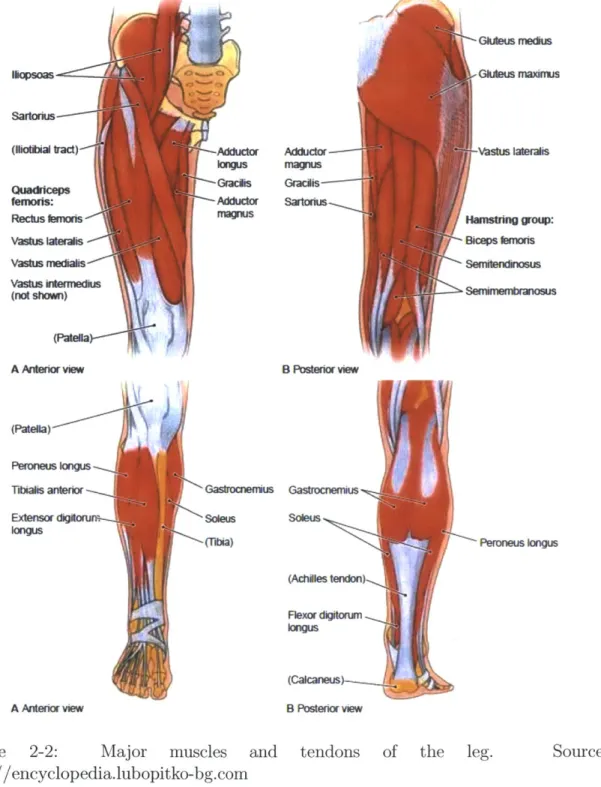
2-2 Major muscles and tendons of the leg. Source: http://encyclopedia.lubopitko-bg.com . . . . 28 2-3 Illustration of the sliding filament theory of muscle contraction. Image
credit: Benjamin Cummings, Addison Wesley Longman, Inc. . . . . . 31
2-4 Flow chart describing neural-structural interactions. Artwork from Cajigas 2009 via Krishnaswamy 2010. . . . . 34
3-1 Metabolic cost of transport is plotted vs. walking speed for each par-ticipant. . . . . 41
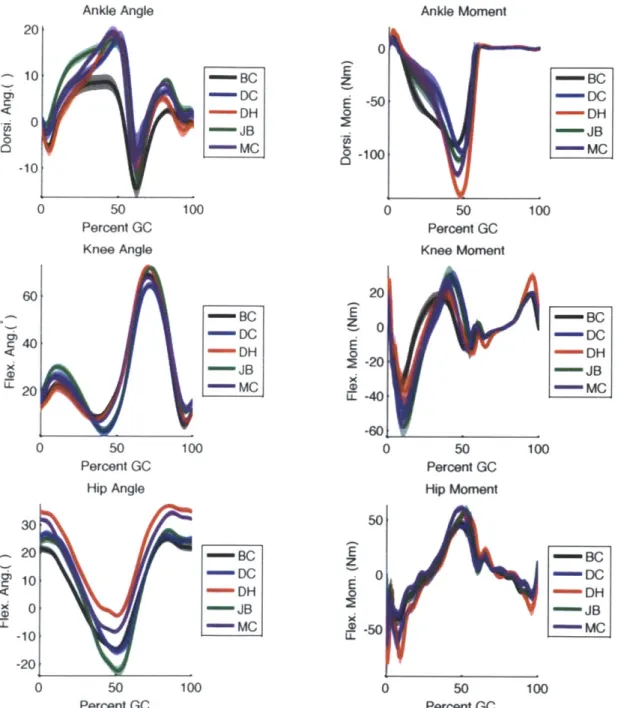
3-2 Ankle, knee, and hip angle and moment trajectories for all subjects walking at 1.25 m /s. . . . . 43
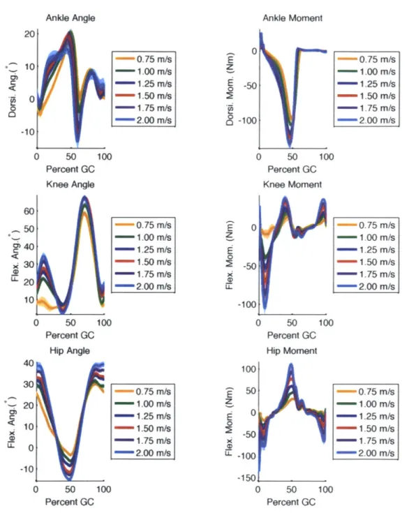
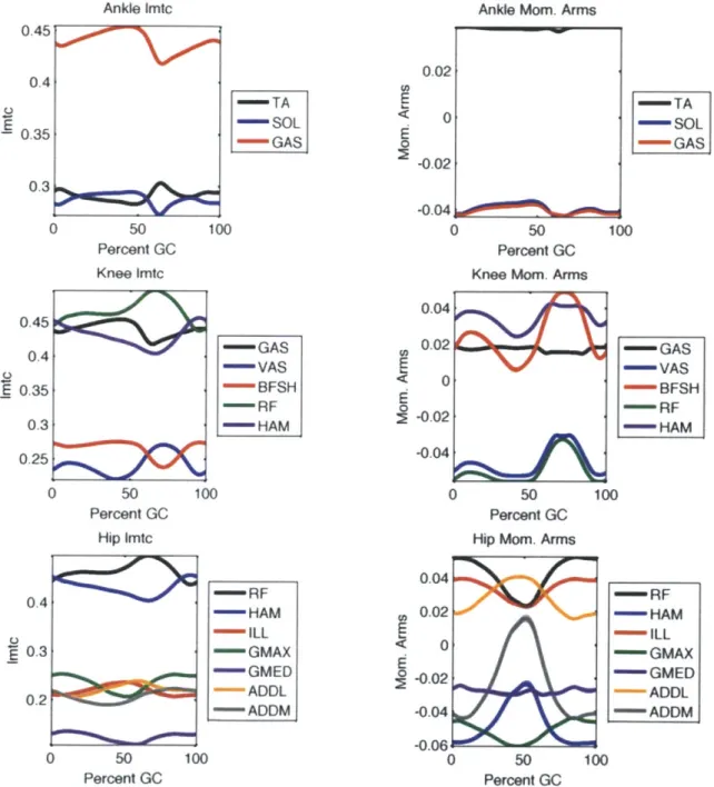
3-3 Variation of ankle, knee, and hip angle and moment trajectories for one subject across speed. . . . . 44 3-4 Muscle-tendon unit lengths and moment arms for one subject walking
at 1.25 m /s. . . . . 45
3-5 Biophysics of muscle activation. Figure credit: Krishnaswamy M.S.
T hesis. . . . . 47
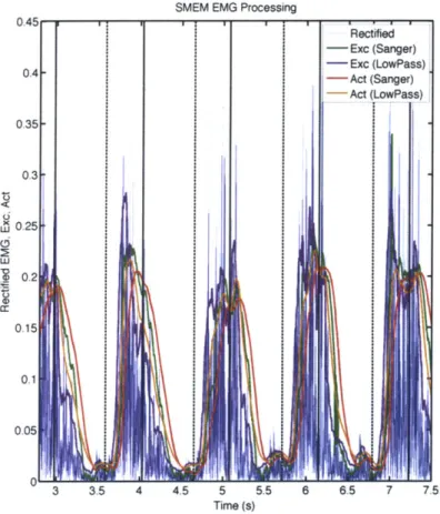
3-6 EMG processing of the semimembranosus (medial hamstring) muscle.
The solid vertical lines are heel strikes of the observed leg while the dashed vertical lines are toe off events. . . . . 51
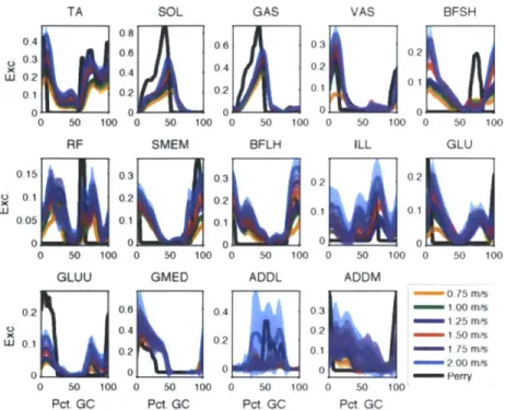
3-7 Mean neural excitation trajectories across speed for all subjects with
reasonable profiles. The estimates were obtained via the Sanger Bayesian method and are compared to the literature values in Perry's Gait
Anal-ysis [421. . . . . 52
3-8 Mean activation trajectories across speed for all subjects with reason-able profiles. The estimates were obtained using the Sanger Bayesian m ethod. . . . . 52
3-9 System model. Note that the soleus and gastrocnemius tendons were modeled separately in the final iteration . . . . 55
3-10 Muscle-tendon system identification procedure . . . . 59
3-11 Empirically motivated metabolic cost function from [35]. . . . . 62
3-12 Typical solution space for optimization problem. . . . . 66
3-13 Metabolic budgets for all subjects plotted vs. kinetic agreement. The vertical line in each plot represents the chosen cutoff point. Here hip muscle excitations were estimated using only collected EMG data. . 68 3-14 Metabolic budgets for all subjects plotted vs. kinetic agreement. The vertical line in each plot represents the chosen cutoff point. Here litera-ture values [42] were used to estimate neural excitations in the monoar-ticular muscles spanning the hip. . . . . 69
3-15 Best solution for each participant and its relation to measured MCOT (light gray band) and MCOT range for all participants (dark gray band). Here hip muscle excitations were estimated using only collected E M G data. . . . . 71
3-16 Best solution for each participant and its relation to measured MCOT (light gray band) and MCOT range for all participants (dark gray band). Here literature values [42] were used to estimate neural excita-tions in the monoarticular muscles spanning the hip. . . . . 72
3-17 Total of all solution spaces. The top plot was formed using hip muscle
excitations derived exclusively from EMG data while the bottom plot was formed using literature profiles
[42]
to estimate neural excitations for the monoarticular muscles spanning the hip. . . . . 733-18 Contributions of individual muscles to joint torques for one subject. . 75
3-19 Muscle fascicle length and velocity trajectories for one subject. . . . . 77
3-20 Comparison of modeled fascicle lengths to trajectories measured via
ultrasound. . . . . 78
3-21 MTU, muscle, and tendon powers for all muscles. In the figures the
black traces are the muscle-tendon unit power outputs, the blue traces are the muscle power outputs, and the red traces are the tendon power outputs. ... ... 79
4-1 (a) Musculoskeletal model applied in prosthesis controller. The two plantar flexors are modeled as muscle-tendon complexes while the dor-siflexor is modeled as a unidirectional rotary spring-damper. (b) Block diagram describing an individual reflex-based controller. The input is composed of joint angles 0 (ankle and knee for GAS; just ankle for
SOL) and the output is the muscle contribution T to ankle torque.
The four blocks represent the geometrical mapping from angle to 1mtc and ankle moment arm (Geom) , the reflex structure (Reflex) , the
stimulation-to-activation dynamics (Eq. 3, block Stim-Act), and the Hill-type muscle model [21],[17] (Hill). . . . . 87
4-2 Gastrocnemius activation, force, contractile element length, and con-tractile element velocity estimated by the data-driven muscle-tendon model. Only stance phase is shown, with zero percent gait cycle rep-resenting heel strike (as is the case in subsequent figures). . . . . 94
4-3 Labeled photograph of the prosthetic apparatus and associated labeled schematic and control architecture. The rotary elements in the ankle-foot prosthesis are shown as linear equivalents in the model schematic for clarity. In the control schematic the parallel spring contribution to prosthesis ankle torque, rp, was subtracted from the desired ankle torque command from the neuromuscular model, Td, to obtain the
de-sired SEA torque Td,SEA. A motor current command imot was obtained by multiplying by the motor torque-constant Kt and produced using
a custom motor controller (not shown). The knee clutch was engaged via the solenoid depending on knee state as obtained from the knee potentiom eter. . . . . 100
4-4 Comparison of the soleus muscle dynamics produced by EMG vs. those produced by reflex feedback to the muscle-tendon model. The top plot shows the contributions from the force, length, and velocity terms to the stimulation. Here the stimulation is the solid line, the force term is the dashed-dot line (largest contributor), the length is the dashed line, and the velocity term (which goes negative) is the dotted line. On the rest of the plots the dashed curves are the model outputs given EMG-based activation, while the solid curves are the corresponding variables when the model activation is determined by the reflex structure in (3). The shaded regions indicate the times where the force, length, and velocity feedback terms contribute at least 0.01 to the stimulation. All plots used biological angles for walking trials at 1.25 m/s. . . . . 101
4-5 Plot of soleus muscle dynamics produced by the reflex-based stimula-tion (Eq. 3) for input ankle angles from walking trials at 0.75 m/s. The top plot shows the contributions to the stimulation (solid line) from the force (dashed-dot line), length (dashed line), and velocity terms (dotted line). The remaining plots (from top to bottom) show the total activation, muscle force, contractile element length, and con-tractile element velocity. The shaded regions indicate the times where the force, length, and velocity feedback terms contribute at least 0.01 to the stim ulation. . . . . 102
4-6 Comparison of prosthesis ankle and knee angles and torques during the clinical trials (measured) with those from a height and weight matched subject with intact limbs (biological). Torque that plantar flexes the ankle is defined to be positive and moves the angle in the positive direc-tion. Similarly torque that flexes the knee is positive and increases the knee angle. The biological values are the thick solid lines (with shaded errors) in each plot while the dashed lines are the values measured on the prosthesis. In the ankle torque plot the commanded torque is shown as a thinner solid line, again with shaded error bars. The knee torque plot compares the torque provided by the clutch-spring mecha-nism to that provided by the natural gastrocnemius in simulation. The vertical line indicates toe off in each plot. . . . 103
4-7 Commanded ankle angles, torques, and workloops for three speeds in clinical walking trials. Shown are data for three speeds: 0.75 m/s (solid line), 1.0 m/s (dashed line), and 1.25 m/s (dotted line). In the torque vs. angle plot heel strike is indicated with by a circle. . . . . 104
4-8 Energy output of the ankle across gait speed. Shown are biological data, net work as commanded by the ankle-foot prosthesis during clin-ical trials, and measured net work during the clinclin-ical trials. . . . . . 105
5-1 Reflex-based forward dynamic walking model. Figure credit: Geyer-Herr 2010 [21]. . . . .111 5-2 Full control paradigm for a biomimetic prosthetic leg controlled by a
List of Tables
3.1 Relevant characteristics of study participants. . . . . 38 3.2 Muscle-specific model parameters. Muscle fiber compositions, w, Tact,
and rdeact were taken from [52]. . . . . 55 3.3 Parameter bounds for optimization problem. . . . . 64 3.4 Optimization settings in MATLAB. . . . . 65 3.5 Cutoffs used to determine optimal solutions and the muscles they were
based upon. . . . . 70 3.6 Metabolic cost estimates from data and both versions of the model.
The first model column uses monoarticular hip excitations from the data while the second uses profiles from [42]. . . . . 74
4.1 Specifications for the ankle-foot prosthesis. The ankle transmission ra-tio took its minimum value at maximum (17 degrees) dorsiflexion and maximum value at maximum (24 degrees) plantar flexion. The series spring stiffness is direction dependent. The reported spring constants are nominal values. In practice they vary with angle and applied torque as governed by the geometry of the linkage and series spring design. However, these variations were experimentally evaluated and subse-quently calibrated out. . . . . 94 4.2 Boundaries and fit values for plantar flexor muscle-tendon and reflex
parameters. The muscle-tendon parameters were determined as de-scribed in [35] and fixed during reflex parameter fitting. . . . . 99
A. 1 Relevant characteristics of all participants from whom EMG data were
recorded. Note that Min. MCOT Speed was only estimated from metabolic data for subjects DH, MC, JB, BC, and DC. It was estimated
using subject preference for participants AD, AM, EM, and DS. . . . 116 A.2 Muscles with reasonable EMG profiles for each subject. Note that
GMED, ADDL, and ADDM were not collected on AD, AM, EM, or DS.116 A.3 r values for LOOCV. The six values in each array refer to walking
at 0.75 m/s, 1.00 m/s, 1.25 m/s, 1.50 m/s, 1.75 m/s, and 2.00 m/s, respectively. No values were computed for ADDL because there was only one set of reasonable measurements of that muscle. . . . . 117
Chapter 1
Introduction
Bipedal walking relies upon a complex interplay of several different physiological systems. The nervous system directs muscle contraction while receiving feedback on muscle force and state. The muscles actuate the skeleton through elastic structures known as tendons. The skeleton interacts with the environment, which is in turn sensed by the nervous system. This highly coordinated network relies on the function of many different neural and structural components. In this thesis we focus on the latter, evaluating the role of tendon compliance during locomotion.
Tendons vary in shape, size, and function depending on the requirements of the muscles to which they are attached. As the interface between muscle and bone, their properties determine how muscles move. Muscle force, state, and metabolic consump-tion are all affected by the structural properties of tendon, yet these properties are rarely evaluated in depth. Here we show how proper consideration of these elastic elements can lend insight into the roles of individual muscles during walking as well as improve metabolic cost predictions. We build a data-driven model of human walking that emphasizes the role of compliance and then apply it in the control of a robotic ankle-foot prosthesis.
1.1
Context
Many different approaches have been taken to model human walking. On one side of the spectrum are purely mechanical systems, such as inverse pendulum walkers and passive dynamic robots [48, 11]. In many cases these systems are able to reproduce the gross mechanical features of gait, but must be properly tuned and do not address the sources of skeletal actuation. On the other side are large scale dynamic optimizations
[3, 39], which seek to model as many muscles of the leg as possible. These models
make some successful predictions but typically significantly overestimate metabolic consumption. The model presented in this thesis represents a middle ground between these two extremes. Below we discuss some previous modeling efforts so as to lend context to the current approach.
1.1.1
Inverse Modeling
Inverse models of locomotion use kinematics measured from motion capture studies to elucidate neural coordination and/or structural features of the leg during walking. Neural coordination has typically been studied through large scale models [3, 39]
that replicate the anatomy of the leg as fully as possible. These models include upwards of fifty leg muscles and dynamically optimize to infer muscle activations. While sophisticated they typically significantly overestimate the metabolic cost of walking (by 47% in [3]), likely because they do not carefully model neural-structural interactions. They use stock values for the parameters governing tendon function, failing to capture variation among subjects. These models also do not thoroughly address the issue of redundancy in joint actuation; for a given movement there are many different combinations of muscle function which could produce the same joint torque.
Another inverse modeling approach is to infer muscle-tendon structure through mechanical approximations to muscle function. Endo et al [19] built a model that uses clutch-spring units in place of most of the major muscles of the leg. This amounts to the assumption that muscles operate isometrically when activated, which is known to
be energetically efficient [53]. While simple, the Endo model is able to reproduce the kinetics and energetics of human walking. However it cannot be used to explore the interaction of neural and structural elements as both are included in the clutch-spring units.
Krishnaswamy et al [35] have successfully explored the interaction in question for the human ankle during walking. They use EMG data to estimate muscle activa-tion and a kinematically clamped optimizaactiva-tion procedure to infer the muscle-tendon morphologies of the muscles spanning the ankle. Their results suggest that proper scaling of the parameters governing tendon function is essential for inferring muscle force, state, and metabolic consumption. In this thesis we refine the method of [35] and extend it to the full leg.
1.1.2
Forward Modeling
Forward dynamic models of locomotion assume neural control schemes in order to produce walking given a set of initial kinematic conditions. One such model is the reflex walker of Geyer and Herr [21], which relies on physiologically-motivated guesses of linear reflex loops. While neural control is known to include both feedforward and feedback components, this model is able to produce stable, terrain adaptive walking using only feedback. An extension of the model [47] produces speed adaptive behavior
by tuning reflexive control parameters. While intriguing, these models are hard to
verify against ground truth as their hypothesized neural pathways are difficult to val-idate. They also use stock parameters to describe tendon force-length characteristics, implying that they would benefit from a means to scale to individual subjects.
1.1.3
Application to Prosthesis Control
Recently forward dynamic, reflex-based neuromuscular models have been applied in the control of robotic limbs [17]. Feedback-based control schemes lend themselves naturally to prosthesis control as they rely only on inputs that may be derived from the on-board sensors of the device. In [17], Eilenberg et al used a simplified version
of the model in [21] to control a robotic ankle-foot prosthesis. They observed ter-rain adaptive behavior, supporting the idea that controllers based on neuromuscular models can produce biomimetic behavior in robotic limbs.
1.2
Research Objectives
This thesis addresses both scientific and technical objectives. On the scientific side we employ a data-driven approach to estimate the force and state of individual muscles during walking. This is accomplished through the combination of two methods; a hidden state estimation of muscle activation and a system identification of optimal muscle-tendon morphologies. The latter procedure is based upon the hypothesis that the muscle-tendon morphology of the human leg has evolved to minimize the metabolic cost of walking at self-selected speed.
Once a realistic muscle-tendon morphology has been obtained, it may be paired with a reflex-based neural control scheme to produce a forward dynamic model. Such a model may be applied in the control of robotic limbs, and here we apply it to a robotic ankle-foot prosthesis. We evaluate the performance of the control scheme across speed, looking for adaptive behavior.
1.3
Thesis Outline
In Chapter 2 we provide the biomechanical and physiological background information necessary to place this thesis in context. We outline the gross mechanics of human walking, describe the biophysical processes that lead to muscle force generation, and discuss the interactions among neural control, muscle contraction, and muscle-tendon structure. We finish with a more precise statement of the problems to be addressed
by this thesis.
In Chapter 3 we present the optimization procedure used to estimate the optimal muscle-tendon morphology of the leg. We discuss data collection and processing techniques, estimation of muscle activation, identification of optimal muscle-tendon
parameter sets, results, and implications of the model.
In Chapter 4 we present a pilot application of our modeling techniques to hardware control, in this case a powered ankle-foot prosthesis. We demonstrate the potential of reflex-based control schemes by observing speed adaptive walking behavior in clinical trials with a bilateral transtibial amputee.
Finally, we discuss the results from a global perspective and address current and future work in Chapter 5.
Chapter 2
Background
Studies of human locomotion apply concepts from several different fields. In this chapter we review the components that are critical to this thesis- the biomechanics of walking, the biophysics of muscle force generation, and the interaction between neural control and muscle-tendon structure. We conclude with a more precise statement of the problems to be addressed by this work.
2.1
Human Walking
The following is a brief introduction to the biomechanics and energetics of human walking. For a more thorough treatment see [42].
2.1.1
Gait Cycle
Human walking is a cyclic motion with a period known as the gait cycle. The gait cycle is defined as the time between consecutive heel strikes (or initial ground contacts) of the same foot. We refer to the time when the relevant foot is on the ground as
"stance" phase and the time when that foot is in the air as "swing" phase. In walking stance phase lasts for more than half the gait cycle (about 60% at self-selected speed), leading to a double support phase in late stance. Further divisions of the gait cycle and their functionality are discussed in [42] and are shown in Figure 2-1.
Divisions of the Gait Cycle
Figure 2-1: Phases of the gait cycle. Figure is reproduced from
[42].
2.1.2
Energetics
Energy consumption during walking comes from the need to move the body forward in a gravitational field. To accomplish this, work must be done on the skeleton by the muscles, which requires metabolic energy. The amount of metabolic energy needed has a quadratic dependence with speed, monotonically increasing from slow walking speeds to fast[3]. The metabolic cost of transport (MCOT) is defined as this energy divided by the distance travelled divided by body weight and forms a concave-up parabola with walking speed. The speed at which the minimum occurs is typically in the range of 1.2 m/s to 1.6 m/s and is very close to the subject's self-selected walking speed, leading researchers to believe that human gait is tuned to minimize MCOT.
2.2
Muscles of the Leg
There are more than fifty muscles used to actuate the legs of the human body [3]. Of these muscles we are primarily interested in those that move the leg in the sagittal (front-back) plane, and specifically those that provide significant torque contribu-tions normal to this plane during walking. Some of these muscles span only one joint (i.e. the soleus actuates only the ankle) while others span two joints (i.e. the ham-strings actuate the knee and the hip). The former group of muscles is referred to as monoarticular while the latter is called biarticular.
Representative drawings of the major muscles of the leg are displayed in Figure 2-2. At the ankle we evaluate the soleus (SOL), gastrocnemius (GAS), and the tibialis anterior (TA) muscles. The first two of these are on the posterior (back) of the leg, are joined by the Achilles tendon, and serve to extend the ankle.1 The soleus spans only the ankle, while the biarticular gastrocnemius actuates both the knee and the ankle. The tibialis anterior is a smaller muscle and is located on the anterior (front) of the shin, serving to flex the ankle.
At the knee we once again include the effects of the gastrocnemius as well as two monoarticular and two other biarticular muscles. The monoarticular knee extensors are comprised of the powerful vastii (VAS) group, while the monoarticular knee flexor is the much weaker biceps femoris short head (BFSH). Two other biarticular muscles span both the knee and the hip; on the anterior side there is the rectus femoris (RF; an extensor) while on the posterior side there is the hamstring (HAM) group. The hamstrings are comprised primarily of the semimembranosus (SMEM), biceps femoris long head (BFLH), and semitendinosus (STEN) muscles which together play a large role in actuating both the knee and the hip.
At the hip, the rectus femoris serves as a source of flexion torque while the ham-strings provide extension torque. In addition to these the hip is actuated by several monoarticular muscles. Since the hip requires fuller three dimensional actuation than the knee and ankle, many of its muscles act in more than one plane. Promoting
'At the ankle, extension is often referred to as plantarflexion and flexion is referred to as dorsi-flexion.
'-Gklueus mecius Adduclor ---magnus Gracis--Sartorius Gktwu rnaximfus Vastus laleralis Hanshilng grou: Biceps bfmoris Sernitendinosus B Posterior view Sarktnus (lIioti bradt)-Ahtu Mtnoriw Perones ~nu vastus Waerafts Vastus medialis \ Vastus intermedius (not shoi) A Anterior view (Patella) Peroneus kXu Tibiais anterior Extensor dgt A Anterior view
Figure 2-2: Major muscles and tendons of http://encyclopedia.lubopitko-bg.com
the leg. Source:
Adducior ons '-Gracis Adduckir magnus Gastrocnemius Soieus (Achiles tendon)-Flexor digitorum 109vus (Cakaneus)--, B Posterior view Gasbacnemus) I solews " (Tibia) I
d
movement primarily in the sagittal plane are the flexors (illiacus (ILL), psoas (PSO)) and extensors (lower gluteus maximus (GMAX)). Causing movement primarily in the coronal (left-right) plane but also providing significant torque normal to the sagittal plane are the upper gluteus maximus, gluteus medius (GMED), adductor magnus
(ADDM), and adductor longus (ADDL). The upper gluteus maximus and gluteus
medius primarily move the leg outward, or abduct the hip. Conversely the adductors move the hip in toward the center of the body. During walking the hip abductors and the adductor magnus provide extension torque normal to the sagittal plane while the adductor longus provides flexion torque.
2.3
Muscle Physiology
In this section we briefly describe the structure of muscles and mechanisms by which they generate force.
2.3.1 Structure
Muscles are the biological motors that actuate the skeleton, enabling motion. They are tension actuators connected to bones by tendons, which are nonlinear elastic structures. The muscle-tendon unit has a net length and velocity that is determined
by the orientation of the joints they span and thus may be inferred from motion
capture data. More information is needed to determine the individual lengths of the muscle and tendon.
Muscles themselves are comprised of several well-defined sub-units. Going from large to small these divisions are muscles, fascicles, fiber bundles, fibers (i.e. cells), myofibrils, myosin, and actin filaments. The actin (thin filaments) and myosin (thick filaments) are arranged in a hexagonal manner.
2.3.2
Contraction Dynamics
Muscle contraction dynamics are controlled by the nervous system through action potential trains delivered to the alpha motor neuron. These action potentials are conveyed to the neuromuscular junction through the axon of the alpha motor neuron via activation of voltage-gated sodium channels. The arrival of the pulse train at the neuromuscular junction prompts an influx of Ca2+ ions through voltage-gated calcium channels. The incoming Ca2+ ions cause the plasma membrane to release acetylcholine into the extracellular space, which in turn activates nicotinic acetylcholine receptors on the neuromuscular junction. This activation opens the intrinsic sodium/potassium channels of the junction, allowing sodium to rush into the muscle cell and potassium to filter out.
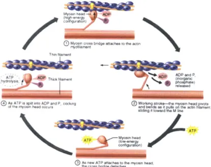
This flow of ions results in an action potential which propagates through the cell via transverse tubules, depolarizing the interior of the muscle fiber. The depolariza-tion wave affects the membranes of the sarcoplasmic reticula, causing them to release calcium ions into the interior of the cell. This calcium binds to the troponin C of the thin filaments, allowing the troponin to allosterically modulate the tropomyosin. In resting muscle the tropomyosin sterically blocks myosin binding sites on the actin fil-ament, but this modulation allows the tropomyosin to move and thereby allow access to the actin filament. Myosin then binds to these sites (in the "strong" state), forming cross bridges and releasing energy stored by the myosin. The myosin subsequently relaxes, rotating its globular head while releasing ADP and inorganic phosphate. This allows the filaments to slide past each other longitudinally and the muscles to con-tract. ATP then binds to the myosin, causing actin to be released and the myosin to be in the "weak" binding state. The ATP is subsequently hydrolyzed by the myosin, moving back to the "cocked back" formation seen at the start of cross bridge forma-tion. The process then repeats as long as ATP and calcium are present near the thin filament. For a visualization of this sliding filament process see Figure 2-3.
Once the action potentials stop firing, the Ca2+ ions leave the troponin molecules and are taken back into the sarcoplasmic reticulum. The tropomyosin reverts to its
K
GMon nos bridge awactes to the actin
A bpd~ ADP aridr t l P,
ATP
,hthelsi phosphate)tche
Copyngt 62001 Beiamo n Cummags an pnnt at Addison Woah-e Longrnan. t,.
Figure 2-3: Illustration of the sliding filament theory of muscle contraction. Image credit: Benjamin Cummings, Addison Wesley Longman, Inc.
resting state and the binding sites on the actin once again become blocked, halting muscle contraction.
2.3.3 Muscle Force Generation Models
Models of the contraction dynamics specified above take many forms, depending on the goals of the problem at hand. Famous isotonic release and thermodynamic
experiments by A.V. Hill
[25]
and others have indicated that muscle force generationmay be modeled in terms of a neural command, the muscle length, and the muscle velocity. The origins and specific definitions of these three inputs are as follows:
Activation: Muscle activation reflects the neural input to a muscle, which can
mod-ulate contraction through the release of calcium ions from the sarcoplasmic reticulum. It is defined as the relative amount of calcium bound to troponin in a muscle, and therefore is a quantity averaged over many muscle fibers. As defined it ranges from 0 to 1, with higher values indicating more potential for cross bridge formation and higher muscle forces.
Length: The length of a muscle affects its output force due to the sliding of filaments
discussed above as well as the passive elasticity of the muscle fibers. The result of the former is bell-shaped active force-length relation (stemming from the formation of cross bridges) which scales with activation. The result of the latter is a quadratic increase with length, independent of activation.
Velocity: The velocity dependence of muscle force stems from the finite amount of
time that cross bridges take to form; if the filaments contract too rapidly fewer cross bridges will form and less force will be generated. On a macro scale this resembles a muscle "viscosity," with the muscle output force decreasing as the fiber shortens more rapidly.
The effects of these three inputs are known to be multiplicative and nearly sepa-rable [56], with the contractile element force FCE being given by
FCE (t) = (t)fA(CE(t))fv(VCE(t))- (2.1)
Here a is activation, fA(lCE(t)) is the active force-length relation, and fv(vCE(t)) is
the force-velocity relation. The passive aspect of the force-length relation is known as the parallel elasticity and it provides an additional contribution FPE, with the total muscle force then being
Fm(t) FcE) + FPE (t) -(2.2)
It should be noted that more sophisticated muscle models exist that do not assume the separability of the activation, force, and velocity terms. However, as was the case with this study, the small performance gains that may be derived from these models often do not justify their additional complexity.
2.4
Tendon Physiology
As mentioned above, tendons are elastic structures that connect muscle to bone. They act in series to the muscle actuators and are connected at oblique angles known as
pennation angles. They are passive and are composed of parallel arrays of collagen fibers, with a dense regular piece of connective tissue encased in a dense irregular outer sheath. Tendons come in various shapes and sizes, depending on function. The largest and strongest tendon in the body is the Achilles, which connects the soleus
and gastrocnemius to the base of the foot.
The force-length curve of tendons is non-linear and can be modeled as an offset exponential. Its slope (the tangent modulus of elasticity) increases for low strains (in the so-called "toe" region) and remains approximately constant for high strains. The curve can be fit using four parameters- a slack length, a reference strain, a shape factor, and an overall scaling factor. These parameters are further discussed in Section 3.1.4. While most models (including ours) assume tendon action to be lossless, it should be noted that studies of animal tendons show losses of 6% - 11% of
stored energy due to viscous effects while shortening at physiological rates [60, 56].
As the intermediary between force sources (muscles) and load (the skeleton), ten-dons play a large role in movement. They determine the impedance seen by the muscles while modulating the force seen by the load.
2.5
Neural- Structural Interactions
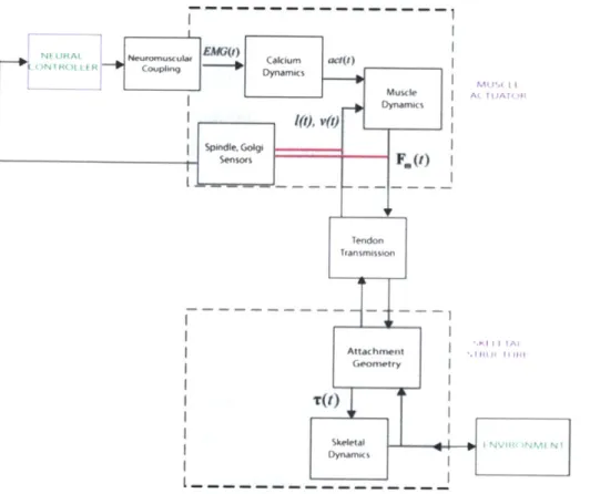
The interactions of the neural controller, muscle actuator, and skeletal "plant" are summarized in Figure 2-4. The nervous system controls the driving signal seen by the muscles. The muscles then act through the tendons to actuate the skeleton and negotiate the environment as desired. The properties/morphologies of the tendon are critical, as they determine the muscle lengths and velocities required to produce the desired output behavior. Tendons allow muscles to both operate with high metabolic efficiency 2 and to regulate their force and state, which are then communicated to the
neural controller via reflexive feedback. This interplay may be understood through the lens of muscle impedance modulation. The nervous system conveys "intent" to
2Muscle metabolic consumption is largely a function of muscle velocity, as will be discussed in
Mucl AiTI) TfI gas ~ ~ ~ ~ 209vaKrsnsam)00~ 1) Spindle. vo gi senso F.(0) Tendon 2ransmssion Attachirmentt Gerometry)fl(IiI
Figure 2-4: Flow chart describing neural-structural interactions. Artwork from
Caji-gas 2009 via Krishnaswamy 2010.
the muscles while etendons produce a "feel" for the environment. The intermediary between the two is muscle impedance, which may be evaluated by studying muscle
force and state.
2.6
Neural Control and the Role of Reflexes
Human motor control is believed to be composed of both a feedforward neural drive and a reflexive feedback component [33],[55]. As shown in Figure 2-4, reflexes dynam-ically link muscle force and state to muscle activation. While it is not known what proportion of the neural signal comes from the feedforward signal and how much comes from the feedback signal, models controlled with only local reflexive feedback loops have been shown to produce walking simulations that qualitatively agree with
human gait dynamics and muscle activations [21].
Having a neuromuscular model driven by only feedback would be useful for con-trolling robotic prosthetic limbs. In this application there is no feedforward driving signal, but the joint state of the prosthesis may be sensed and fed back to the con-troller. The joint state can be mapped to muscle-tendon length, which, when com-bined with a reflex structure, can be used to drive a muscle model. The output forces of the muscle model would then be mapped to desired torque of the device, allowing the loop to be closed. Eilenberg et al
[17]
observed terrain adaptive behavior when applying this method to control a robotic ankle foot prosthesis.2.7
Problem Statement
This background information provides context for a more precise formulation of our objectives. We seek to build a data-driven model of walking that enables determina-tion of the force and state of each modeled muscle throughout the gait cycle. Doing so would allow us to resolve the contributions of each muscle to joint torque, solving the redundancy problem and providing a basis to investigate neural control strategies. Mathematically we have, at each joint:
T(t) = Fi(t)ri(t) (2.3)
lMTC,i(t) = l,(t) + lm,i(t)cos(Oi(t)) (2.4)
Fi(t) = Fi(t) = Fm,i(t)cos(Oi(t)) (2.5)
Fmi (t) cC a (t)f1(lCE,i (t))f(vCE,i (t)) + FPE (lCE,i (t)) (2-6)
F,i(t) = ft'i(lt,1, '-i) (2.7)
Assuming that the muscle-tendon lengths lmtc,i can be estimated from geometry, the remaining unknowns are the muscle activations ai(t), muscle states 1CE,i (t), and
state ac(t) using EMG data. We then hypothesize that the human body has evolved to minimize the metabolic cost of walking at self-selected speed. We apply this hy-pothesis to determine the unknown muscle-tendon morphologies MiZ and muscle states
1
CE,i(t), evaluating the results against empirical studies. The methods and results of
this inverse optimization problem are presented in the next chapter.
Once this inverse problem is solved, the results may be applied in the control of robotic limbs. In Chapter 4 we discuss how an optimal reflex structure was wrapped around this model and used to control a powered ankle-foot prosthesis.
Chapter 3
Muscle-Tendon Morphology
Optimization
As previously described, neuromuscular walking models may be improved by plac-ing a greater emphasis on the role of compliance. Here we describe a method for obtaining more accurate metabolic cost and muscle state estimates by determining the muscle-tendon morphology for an individual human. To achieve this we first col-lected kinematic, kinetic, electromyographic, and metabolic data from five subjects. The kinematic data were used to estimate muscle-tendon states and moment arms, the kinetic data were used to estimate joint moments, and the EMG data were used to estimate muscle activation. We performed a kinematically-clamped, multi-objective optimization of the parameters that govern the force-length curve of each tendon, searching for parameter sets that simultaneously matched the collected kinetic data and minimized metabolic cost. In the following sections the specifics of this method as well as its results are discussed.
Subject Age Mass Leg Length Ethnicity Sport Min. MCOT DH 24 80.3 kg 0.953 m African Basketball 1.32 m/s MC 24 72.3 kg 0.927 m Caucasian Running 1.49 m/s JB 29 68.9 kg 0.933 m Caucasian Running 1.31 m/s BC 26 65.0 kg 0.902 m Caucasian Running 1.38 m/s DC 25 65.4 kg 1.028 m Caucasian Running 1.47 m/s
Table 3.1: Relevant characteristics of study participants.
3.1
Methods
3.1.1
Data Collection
Kinematic, kinetic, electromyographic, and metabolic data were collected from five adult males in a study approved by the MIT Committee on the Use of Human Subjects and conducted at the Harvard University Skeletal Biology Lab. The heights, weights, ethnicities, and favorite sports of the study participants are listed in Table 3-1. All subjects were male and of at least moderate athletic ability, with the runners all being at a semi-professional level. This group was chosen because EMG signals recorded from participants with athletic backgrounds are typically cleaner than those obtained from sedentary individuals. All subjects were pre-screened to avoid gait pathologies and current injuries. Further details on each data modality are as follows:
Metabolic Data The required data sets were collected in two phases. After
in-formed consent was obtained, the subjects were first outfitted with a portable oxygen consumption mask attached to a Cosmed K4B2 V0
2 system. This system employs a standard open-circuit gas analysis technique to estimate metabolic energy consumption based on measurements of oxygen inhaled and exhaled [7]. The subjects' were then asked to stand still for'seven minutes while a basal measurement was recorded. They then walked barefoot on an instrumented treadmill for seven minutes at each of six speeds (0.75 m/s, 1.00 m/s, 1.25 m/s, 1.50 m/s, 1.75 m/s, and 2.00 m/s), allowing the variation of metabolic energy expenditure to be measured across speed. These results were
quickly tabulated and used to estimate the walking speed where the metabolic cost of transport (MCOT) was minimal (Table 1).
Once the metabolic cost measurements were completed, the oxygen consump-tion mask and Cosmed system were removed and the participants were outfitted for the second phase. In this second phase kinematic, kinetic, and electromyo-graphic data were collected for two minutes of barefoot walking at each of seven speeds; the six listed above and the speed where the subject's MCOT was found to be minimal. The methods for collecting these three data types were the fol-lowing:
Kinematic Data An infrared camera system (8 cameras, Qualisys Motion Capture
Systems, Gothenburg, Sweden) was used to track the motion of subjects as they walked in the capture volume. Reflective markers were placed at 43 (bilateral) locations on the participant's body and their three dimensional trajectories were recorded at 500 Hz. The marker locations were chosen specifically to track joint motion, as prescribed by the Helen Hayes marker model.
Kinetic Data An instrumented force plate treadmill (Bertec Corporation,
Colum-bus, OH) was used to measure the ground reaction forces of the subjects as they walked. Foot contact centers of pressure were also recorded. The treadmill had two side-by-side belts, ensuring that each foot would be measured separately.
The sampling rate for these observations was 1000 Hz.
Electromyographic Data A surface EMG system (Motion Lab Systems, Baton
Rouge, LA) was used to record activity in fourteen muscles of one leg of each subject (tibialis anterior, soleus, medial gastrocnemius, vastus lateralis, biceps femoris shorthead, rectus femoris, semimembranosus, biceps femoris long head, illiacus, gluteus maximus (lower), gluteus maximus (upper), gluteus medius, adductor longus, and adductor magnus). Symmetry was assumed for the other leg, and all channels were sampled at 1000 Hz. The signals were recorded at the surface using pre-gelled bipolar electrodes (Electrode Store Model BS-24SAF, part number DDN-20) and amplified 20 times by pre-amplifiers (Motion Lab
Systems, part number MA-411). Prior to walking trials a maximum voluntary
contraction (MVC) trial was conducted for each muscle group wherein the par-ticipant was asked to work that particular group as hard as possible. These trials were used for normalization purposes in muscle activation estimates. The second phase was conducted separately from the first for practical reasons; with long trials markers would occasionally become dislodged and the EMG surface connections eventually degraded.
3.1.2
Data Processing Procedures
The following steps were taken to produce the required model inputs and output references.
Metabolic Cost Estimation
The metabolic data were used as both (i) a means to find the walking speed where the MCOT was minimal and (ii) a way to estimate the metabolic cost of walking across speed. As mentioned previously, we hypothesize that the human body has evolved to maximize the metabolic efficiency of walking at a preferred speed, and this "self-selected" speed is taken to be where the MCOT is minimal. Hence the metabolic data determine the speed where the model should be trained while providing target metabolic consumption values for the model to replicate at all recorded speeds.
As mentioned above, our system uses a standard open-circuit gas analysis tech-nique to estimate metabolic energy consumption based on measurements of oxygen inhaled and carbon dioxide exhaled [7]. Specifically, the formula for metabolic energy expenditure in kJ is
Metabolic Energy Expenditure = 20.964VAO2, (3.1)
where V is the ventilation rate (pulmonary or exhaust) and A0 2 is the oxygen
con-centration difference in the inspired and expired air. This equation is known to have an accuracy of ±3%. The metabolic cost of transport (MCOT) is then defined as
Metabolic Cost of Transport vs. Speed 0.5 0.48 " DC IDDH 0.46 --- JB MC 0.44 0.42 0. 0.38 0.36 0.34 0.32 0.3 0.8 1 1.2 1.4 1.6 1.8 2
Walking Speed (mis)
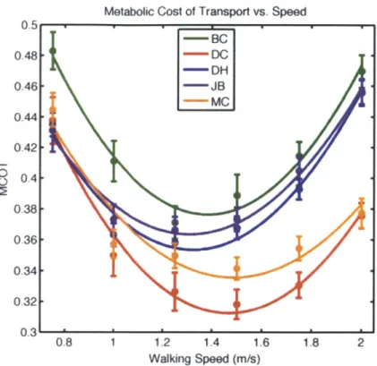
Figure 3-1: Metabolic cost of transport is plotted vs. walking speed for each partici-pant.
Metabolic Energy Expenditure
MCOT Distance Travelled x Body Weight (3.2)
and typically has a minimum value of about 0.35, which occurs at a walking speed in the range of 1.2 m/s - 1.6 m/s. To determine the walking speed where MCOT was
minimal for our participants we used a quadratic fit of the MCOT vs. speed plot, as shown in Figure 3-1. The resulting speeds for each subject are shown in Table 3-1.
Joint States and Moments
To formulate our inverse optimization problem we require joint angle and moment trajectories. These quantities describe motion on a macro scale and may be estimated using the collected motion capture and force plate data. The motion capture data sets are comprised of tracked marker trajectories in 3D space, each representing an anatomical landmark. The force plate data sets include ground reaction force (GRF) vectors and the location of the center of pressure (COP) of each GRF.
After collection, the motion capture trajectories are labelled and have their gaps filled via a spline-based interpolation algorithm in the Qualisys Track Manager (QTM,
Qualisys
Motion Capture Systems, Gothenburg, Sweden) software. The raw force plate data are processed and low pass filtered with a cutoff of 50 Hz in MATLAB (Mathworks, Natick, MA). The two data sets are synced and exported to SIMM (Software for Musculoskeletal Modeling, Musculographics Inc., Evanston, IL).The SIMM software was chosen for this analysis because of its unparalleled anatom-ical accuracy. It provides reasonable, subject-specific representations of body seg-ments, joints, and muscle-tendon units. It also allows the user to access subject-specific parameter scalings, which proved critical for our analysis. SIMM is based on a model of an "average" human body that was formulated through cadaver studies and may be scaled and tweaked for any individual. The scaling is obtained through an inverse kinematic fit to a static trial and is applied in determining the kinematics for each subsequent walking trial. The kinematic output is combined with the force plate data to compute joint torque profiles via inverse dynamics. This step is per-formed by the SIMM Dynamics Pipeline using the SDFAST (PTC, Needham, MA) software.
Several post-processing steps were performed to produce the average torque pro-files that were used in the ensuing analysis. First the data sets were broken into gait cycles as determined by the force plate data. Gross outlier gait cycles were discarded and the remaining time series were normalized in time to percent gait cycle and av-eraged. Plots of typical angle and torque profiles and their variation across speed are shown in Figures 3-1 and 3-2. Note that while SIMM produces a full 3D body representation, only motion in the sagittal (front-back) plane was considered for this model.
Muscle-Tendon States and Moment Arms
To study force production by muscles, we must have a means to estimate muscle-tendon lengths and moment arms. These quantities are related to joint angles through complex musculoskeletal geometry, which is modeled in SIMM using wrap objects.
Ankle Angle 20 10 0 -10 0 50 100 Percent GC Knee Angle 0 50 100 Percent GC Hip Angle 30 20 10 0 -10 -20 0 50 100 Percent GC - BC -DC - DH - JB - MC - BC .. DC - DH - JB - MC z E is E 0 E 0 - BC -DC - DH - JB - MC Ankle Moment 0 -50 -100 0 50 10 Percent GC Knee Moment 20 0 -20 -40 -60 0 50 100 Percent GC Hip Moment 50 0 -50 0 50 100 Percent GC BC -DC - DH - JB - MC 0 - BC - DC - DH - JB - MC - BC -DC - DH - JB - MC
Figure 3-2: Ankle, knee, and hip angle and moment trajectories for all subjects walking at 1.25 m/s. 0a x 02 U-.-(Db M 6( 2(
Ankle Angle 20 -^ 10 0 -10 0 50 10( Percent GC Knee Angle 60 50 40 30 20 10 0 50 104 Percent GC Hip Angle X 2( -0.75 m/s - 1.00 M/s - 1.25 m/s - 1.50 m/s 1.75 m/s - 2.00 m/s E z E 0 28 is 0.75 m/s - 1.00 M/s - 1.25 m/s - 1.50 M/s 1.75 m/s 2.00 m/s z 0 CD z 0 CD M - 0.75 m/s - 1.00 M/s -1.25 m/s - 1.50 m/s -1.75 m/s 2.00 m/s 0 50 10 Percent GC Ankle Moment 0 -50 -100 0 50 10( Percent GC Knee Moment 0 -50 -100 0 50 10( Percent GC Hip Moment 100 50 0 .50 -100 -150 0 50 10( Percent GC -0.75 m/s - 1.00 M/s - 1.25 m/s -- 1.50 m/s - 1.75 m/s - 2.00 m/s 0.75 m/s - 1.00 M/s - 1.25 m/s 1.50 m/s 1.75 m/s - 2.00 m/s -0.75 m/s - 1.00 m/s -- 1.25 m/s -1.50 m/s - 1.75 m/s -2.00 m/s
Figure 3-3: Variation of ankle, knee, and hip subject across speed.
angle and moment trajectories for one
* 0
- TA - SOL - GAS Ankle Imtc 0 ,4 5 , * 0 0.4 0.35 0.3 0 50 100 Percent GC Knee Imtc .45 0.4 3.35
K
0.3-).25 0 50 100 Percent GC Hip Imtc 0.4 0.3 -0.2 0 50 100 Percent GC E 0 E 0 E 0 0 2Ankle Mom. Arms
0.02 01 -0.02 -0.04 0 50 100 Percent GC
Knee Mom. Arms 0.04 0.02 0--0.02 -0.04 0 50 100 Percent GC
Hip Mom. Arms
0.04 0.02 -0 --0.02 -0.04 --0.06 0 50 100 Percent GC -TA - SOL -GAS - GAS - VAS - BFSH - RF - HAM -RF - HAM - ILL -GMAX -GMED ADDL -ADDM
Figure 3-4: Muscle-tendon unit lengths and moment arms for one subject walking at
1.25 m/s. E - RF - HAM - ILL -GMAX -GMED ADDL -ADDM -GAS -VAS "BFSH - RF - HAM
The wrap objects are derived using information from cadaver studies and digitized bone surfaces[15]. The inputs to the applied method are joint angles and SIMM's subject-specific musculoskeletal scaling, which are then used to determine muscle-tendon lines of action and the quantities we seek.
To produce the profiles used as input to the model, we follow the same post-processing steps as were used with joint angles and moments. Specifically we break the time series into gait cycles, discard outliers 2, normalize to percent gait cycle, and average. Plots of typical muscle-tendon lengths and moment arms are shown in Figures 3-3 and 3-4.
3.1.3
Muscle Activation Estimation
The final required input for our inverse optimization problem is muscle activation, which represents the control signal from the nervous system to the muscles. This signal may be estimated using recordings from surface electromyography (EMG). Be-low we recap the biophysical processes involved in muscle activation, the information contained in EMG signals, and the mathematical methods employed in estimating muscle active state.
Biophysics of Muscle Activation
As described more fully in Section 2-3, muscle contraction is initiated by action po-tential trains delivered to the alpha motor neuron. The arrival of this neural signal starts a process that results in the release of calcium ions from the sarcoplasmic reticulum (SR). These calcium ions diffuse through the cell, binding to troponin and enabling cross bridge formation and thereby muscle contraction. Mathematically the release of calcium ions from the SR may be modeled as a rapid jump process, while the spread of calcium through the cell and its binding to troponin may be modeled as a slower diffusion process. Activation is defined as the relative amount of calcium bound to troponin in a muscle (averaged over all cells) and therefore gives a direct
2
The outliers for muscle-tendon length and moment arm were assumed to be the same as those for joint angle/moment, as joint angle can be mapped to the former two quantities.
![Figure 2-1: Phases of the gait cycle. Figure is reproduced from [42].](https://thumb-eu.123doks.com/thumbv2/123doknet/14539831.535290/26.918.185.703.115.510/figure-phases-gait-cycle-figure-reproduced.webp)