The Red Sea Deep Water is a potent source of atmospheric ethane and propane

HAL Id: hal-03109194

https://hal.archives-ouvertes.fr/hal-03109194

Submitted on 21 Jan 2021

HAL is a multi-disciplinary open access

archive for the deposit and dissemination of

sci-entific research documents, whether they are

pub-lished or not. The documents may come from

teaching and research institutions in France or

abroad, or from public or private research centers.

L’archive ouverte pluridisciplinaire HAL, est

destinée au dépôt et à la diffusion de documents

scientifiques de niveau recherche, publiés ou non,

émanant des établissements d’enseignement et de

recherche français ou étrangers, des laboratoires

publics ou privés.

Distributed under a Creative Commons Attribution - NonCommercial| 4.0 International

License

The Red Sea Deep Water is a potent source of

atmospheric ethane and propane

Efstratios Bourtsoukidis, Andrea Pozzer, Tobias Sattler, Vasileios N.

Matthaios, Lisa Ernle, Achim Edtbauer, Horst Fischer, Tobias Könemann,

Sergey Osipov, Jean Daniel Paris, et al.

To cite this version:

Efstratios Bourtsoukidis, Andrea Pozzer, Tobias Sattler, Vasileios N. Matthaios, Lisa Ernle, et al.. The

Red Sea Deep Water is a potent source of atmospheric ethane and propane. Nature Communications,

Nature Publishing Group, 2020, 11 (1), �10.1038/s41467-020-14375-0�. �hal-03109194�

The Red Sea Deep Water is a potent source

of atmospheric ethane and propane

E. Bourtsoukidis

1

*, A. Pozzer

1

, T. Sattler

1

, V.N. Matthaios

2

, L. Ernle

1

, A. Edtbauer

1

, H. Fischer

1

, T. Könemann

3

,

S. Osipov

1

, J.-D. Paris

4

, E.Y. Pfannerstill

1

, C. Stönner

1

, I. Tadic

1

, D. Walter

3,5

, N. Wang

1

, J. Lelieveld

1,6

&

J. Williams

1,6

Non-methane hydrocarbons (NMHCs) such as ethane and propane are significant

atmo-spheric pollutants and precursors of tropoatmo-spheric ozone, while the Middle East is a global

emission hotspot due to

extensive oil and gas production. Here we compare in situ

hydrocarbon measurements, performed around the Arabian Peninsula, with global model

simulations that include current emission inventories (EDGAR) and state-of-the-art

atmo-spheric circulation and chemistry mechanisms (EMAC model). While measurements of high

mixing ratios over the Arabian Gulf are adequately simulated, strong underprediction by the

model was found over the northern Red Sea. By examining the individual sources in the model

and by utilizing air mass back-trajectory investigations and Positive Matrix Factorization

(PMF) analysis, we deduce that Red Sea Deep Water (RSDW) is an unexpected, potent

source of atmospheric NMHCs. This overlooked underwater source is comparable with total

anthropogenic emissions from entire Middle Eastern countries, and signi

ficantly impacts the

regional atmospheric chemistry.

https://doi.org/10.1038/s41467-020-14375-0

OPEN

1_{Department of Atmospheric Chemistry, Max Planck Institute for Chemistry, Mainz 55128, Germany.}2_{School of Geography, Earth and Environmental}

Sciences, University of Birmingham, Edgbaston, Birmingham B15 2TT, UK.3_{Department of Multiphase Chemistry, Max Planck Institute for Chemistry, Mainz}

55128, Germany.4_{Laboratoire des Sciences du Climat et de l’Environnement, CEA-CNRS-UVSQ, UMR8212, IPSL, Gif-Sur-Yvette, France.}5_{Max Planck}

Institute for Biogeochemistry, Hans-Knöll-Straße 10, 07745 Jena, Germany.6_{Energy, Environment and Water Research Center, The Cyprus Institute,}

Nicosia, Cyprus. *email:e.bourtsoukidis@mpic.de

123456789

T

he Middle East accommodates more than half of the

world’s known oil and gas reserves

1

_{. Fossil fuel exploitation}

in this region is responsible for the release of large amounts

of gaseous pollutants into the atmosphere, including methane

(CH

4

)

2

and non-methane hydrocarbons (NMHCs)

3

. Ethane and

propane have the strongest sources

4

_{, and being relatively}

long-lived (ethane ca. 2 months, propane ca. 2 weeks)

5

_{are ubiquitous}

in the global atmosphere. Atmospheric oxidation of NMHCs in

the presence of nitrogen oxides (NO

x

) leads to production of

tropospheric ozone

6,7

_{and peroxyacetyl nitrates (PAN) that are}

phytotoxic

8–10

and harmful to human health

11

. The abundance of

NMHCs and NO

x

in combination with the intense

photo-chemistry in the Arabian Basin results in extremely high ozone

mixing ratios that can reach up to 200 ppb

12

.

Globally, the atmospheric concentrations of ethane and

pro-pane exhibit temporal trends that are closely related to

anthro-pogenic activities. The general decline in fossil fuel emissions

toward the end of the twentieth century resulted in a decline of

global atmospheric ethane and propane

13

_{. Conversely, the}

sub-sequent expansion of US oil and natural gas production has led to

a reversal of their global atmospheric trends, with emissions

increasing since 2010

3

_.

While anthropogenic activities substantially influence the

emission rate and composition of atmospheric hydrocarbons,

Earth’s natural degassing is also a significant source

14

_{. Natural}

geologic (i.e., mud volcanoes, onshore and marine seeps, and

micro seepage, geothermal and volcanic) sources contribute to

both ambient ethane and propane concentrations, and their

inclusion in global emission inventories helps to better explain

the reported values from the expanding global observation

net-work

15

. Indeed such sources will have dominated preindustrial

emissions.

During the AQABA ship campaign, which took place between

July and August 2017, NMHCs were monitored around the

Arabian Peninsula (Supplementary Fig. 1). By comparing

the observations with model simulations, we aim to evaluate the

emission inventories and atmospheric chemistry mechanisms

while focusing on the most abundant anthropogenic

hydro-carbons: ethane and propane. The largest measurement/model

discrepancy was observed over the northern part of the Red Sea,

which was investigated in terms of possible underestimation of

existing sources and emission patterns (i.e., ratios between the

measured hydrocarbons) that are derived by using positive matrix

factorization analysis.

Results and discussion

Observations and model simulations. The atmospheric mixing

ratios of ethane and propane ranged over three orders of

mag-nitude around the periphery of the Arabian Peninsula

(Supple-mentary Figs. 2–4). From their tropospheric background values

over the Arabian Sea (defined as the lowest 10% of data points:

0.18 ± 0.02 ppb for ethane and 0.02 ± 0.01 ppb for propane), to a

maximum of ~50 ppb over the Arabian Gulf, variations in

absolute and relative abundance of the NMHCs indicated

mul-tiple emission sources

16,17

_{. The high mixing ratios over the}

Arabian Gulf and Suez Canal could be attributed to emissions

from the intense oil and gas activities and urban centers,

respectively

16

_{. However, in the region with the second highest}

average abundance, namely the northern part of the Red Sea, the

levels of the measured NMHCs could not be attributed to a

known source

16

_.

To identify the source and to generally evaluate the Middle

Eastern NMHC emission patterns, a state-of-the-art atmospheric

chemistry model (EMAC, ECHAM5/MESSy for Atmospheric

Chemistry)

18,19

was used to simulate the concentrations along the

route. As emission inventory input, we used the most recent

version of the Emission Database for Global Atmospheric

Research (EDGAR v4.3.2)

20,21

_{, which was further upgraded to}

include gas

flare emissions and geothermal sources (see the

“Methods” section).

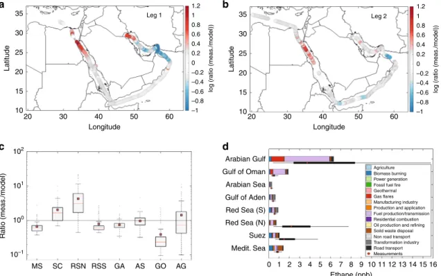
The observed ethane mixing ratios were reproduced by the

model for most of the route (Fig.

1

), indicating that emission

sources and atmospheric processes in the Middle East region are

generally well understood. Significant model underestimations

(Suez Canal, northern Arabian Gulf) and overestimations (Gulf of

Oman) occurred for short periods only during the

first leg of the

route, suggesting local, small-scale inconsistencies in the emission

sources. The only region that was inadequately simulated during

both legs of the route was the northern part of the Red Sea where

measured mixing ratios of ethane and propane were up to about

20 (average ± standard deviation

= 4.3 ± 3.8) and 40 (average ±

standard deviation

= 7.8 ± 5.9) times higher than model

predic-tions. According to the model results, biomass burning, fuel

production and transmission, and transformation industry

emissions regulate the regional hydrocarbon abundance (Fig.

1

d;

Supplementary Fig. 5). However, neither the dominant nor any of

the 15 inventory sources was able to explain the observations,

even when the emission strength was varied (Supplementary

Fig. 6).

Source apportionment. To derive the hydrocarbon signature of

the potent unidentified source, a well-established receptor model

(positive matrix factorization; US EPA PMF 5.0) was utilized

22

_.

Receptor models use ambient observations to apportion the

observed species concentrations to signature sources by assessing

changes in species correlation with time and

finding the optimum

solution that explains the concentrations of all observed

constituents.

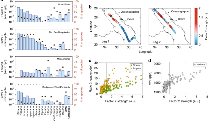
The PMF analysis of the northern Red Sea data identified 4

distinct emission sources/factors (Fig.

2

a). Factor 1 illustrates an

emission source that is rich in C2–C6 hydrocarbons, alkenes and

acetonitrile (a biomass-burning tracer

23

_{), with contributions}

mainly during the

first leg when the air masses originate from

the Suez Canal (Supplementary Fig. 7). In addition, it correlates

with anthropogenic activity markers such as acetone, methanol,

and acetaldehyde (Supplementary Fig. 8), confirming the urban

character of this emission source. By contrast, factor 4 was

significant only during the second leg (Supplementary Fig. 9)

when the air originated from the Sinai Peninsula. The small

concentration contribution and back-trajectory-specific direction

suggest a background signature from a region with small emission

sources. Factor 3 apportions marine traffic emissions that are

clearly distinguishable from the sporadic occurrences

(Supple-mentary Fig. 10), high ethene, large alkanes (>C4), and the

absence of ethane

16

_{in the emission pattern.}

The remaining factor 2 is characterized by exceptionally high

alkane concentrations that decrease with increasing carbon

number. Alkene contribution is negligible, and in combination

with the absence of acetonitrile in the emission signature, factor 2

points toward a non-anthropogenic emission source. The source

contribution to the measured signal is expressed by the

significance of the factor that is termed as factor strength. As

shown in Fig.

2

b, this source contributed most to the

measurements over the northmost part of Red Sea and in

particular between 23° and 27° latitude. Since the model

underestimation (expressed by the ratio between measurements

and models) increases with the strength of factor 2 (Fig.

2

c), it

becomes evident that it represents the missing source.

Summarizing, the high ethane and propane mixing ratios that

were observed over the northern part of Red Sea could not be

explained by the known sources that are included in the emission

inventory (Supplementary Fig. 6). PMF analysis identified the

emission source signature, suggesting that it is distinct from other

known sources, of non-anthropogenic origin, and specific to the

region of the Red Sea. Back-trajectory calculations

(Supplemen-tary Fig. 7) show that the origin of the air masses remained

unchanged along each leg. The highest ethane mixing ratio

underprediction occurred over two hot spots pointing toward a

local source. One possibility is that the missing source of

hydrocarbons is the sea. Marine emissions of NMHCs have been

documented previously

24–26

_{, however,}

_{fluxes were low. If the}

hydrocarbons originate from the sea, then an exponential

relationship between the measured mixing ratios and wind speed

can be expected due to the

flux dependency on wind strength

27,28

_.

Indeed, ethane, propane, butanes, and methane mixing ratios do

display exponential increases with the wind speed that

addition-ally correlates with the model underestimation (Supplementary

Fig. 11). Methane in particular was substantially increased over

the northern Red Sea, with an enrichment (i.e., subtracted

backgrounds) methane to ethane ratios of 93 ± 77, considerably

higher than the respective ratios observed over the Arabian Gulf

(35 ± 23) that represents the high end of oil- and

gas-processing-related ratios

3

_.

Red Sea Deep Water. The Red Sea lies between the Arabian and

African continental plates and has some unique geological

fea-tures. The southern Red Sea

floor has been spreading for the past

5 million years, while the northern part is in a stage of continental

rifting

29

_{. Distinct movements of the tectonic plates have led to a}

partly fractured sea

floor and the formation of numerous

brine-filled pools that are characterized by close-to-solubility limit

halite (mineral form of NaCl) concentrations and strong

tem-perature gradients

30,31

_{. Generally, the water occupying depths}

from 300 to 2000 m in the Red Sea is recognized as the warmest

and saltiest deep water in the world with pronounced

season-ality

32

_{, although the rates and mechanisms of its renewal remain}

uncertain.

Hydrocarbon release from the Red Sea

floor can occur through

direct

fluid seepage from hydrocarbon reservoirs deposited above

offshore rocks, located between 25 and 28°N (e.g., Rudeis and

Kareen formation). In addition, the Gulfs of Suez and Aqaba

contribute to the RSDW through bottom-trapped density

outflows

33

_{. Considering that this region is known for the large}

oil and gas reserves, natural seepage and crude oil/gas seepage

from leaky subsea wells could be a significant submarine source of

NMHCs in this region. Finally, the numerous brine pools that are

located on the sea

floor need to be considered. Depending on

their chemical composition, the brine pools are classified into two

distinct types

31

_{. The formation of Type I brine pools is controlled}

by evaporate dissolution and sediment alteration, characterized

by exceptionally high methane and hydrocarbon concentrations.

Short-chained hydrocarbons are formed by the degradation of

long-chained hydrocarbons that originate from the organic-rich

sedimentary rocks

34

_{and the bioproduction in the brine’s water to}

sediment interface

35,36

_{. Type II brine pools are controlled by}

volcanic/magmatic alterations and are poor in organic material.

They are more common and are frequently found in the southern

and middle part of the Red Sea

floor. In contrast, only two brine

pools are classified as type I: the Oceanographer deep (26°17.2′N,

35°01.0′E)

37

_{and the Kebrit deep (24°43.1′N, 36°17′E)}

38

_.

Oceanographer in particular is known to contain high methane

35

a

b

c

d

30 25 Latitude Ratio (meas ./model) log (r atio (meas ./model)) 20 15 10 102 101 100 MS SC RSN RSS GA AS GO AG 0 1 2 3 4 5 6 7 8 Ethane (ppb) 9 10 11 12 13 14 15 16 10–1 35 30 25 Latitude 20 15 10 Arabian Gulf Gulf of Oman Arabian Sea Gulf of Aden Red Sea (S) Red Sea (N) Suez Medit. Sea 20 30 40 Longitude 50 60 20 30 40 Longitude 50 60 Agriculture Biomass burning Power generation Fossil fuel fire Geothermal Gas flares Manufacturing industry Production and application Fuel production/transmission Residential combustion Oil production and refining Soild waste disposal Non road transport Transformation industry Road transport Measurements Leg 1 1.2 1 0.8 0.6 0.4 0.2 –0.2 –0.4 –0.6 –0.8 –1 0 log (r atio (meas ./model)) 1.2 1 0.8 0.6 0.4 0.2 –0.2 –0.4 –0.6 –0.8 –1 0 Leg 2

Fig. 1 Comparison between ethane measurements and model simulations. Timeline ratios are displayed for both leg 1 (a) and leg 2 (b). In c, geospatial ratio statistics are displayed with the boxplots that illustrate the median with red line and the mean with red squares. The bottom and top edges of the box indicate the 25th (q1) and 75th (q3) percentiles, respectively. The boxplot draws points as outliers if they are greater thanq3 + w × (q3 − q1) or less than q1 − w × (q3 − q1). The whiskers correspond to ±2.7σ and 99.3% coverage if the data are normally distributed. In d, geospatial measured volume mixing ratios of ethane are shown with black boxplots where the red circles are the median measured values and the whiskers are defined as in (c). The modeled mixing ratios are in bars for each emission sector.

concentrations (4921

μl/l

39

(average methane inside type II brines

is 0.04 ± 0.04

μl/l))

31

_{and it is located directly underneath the}

region with the highest discrepancy between NMHC

measure-ments and model simulations. The mixing between the dense

brine pools and RSDW occurs via diffusion across the strong

salinity gradient, and the reported methane emissions are

relatively weak with values up to 393 kg/yr for the Kebrit deep

40

_.

However, the impact of above-brine water currents that may

enhance the

fluxes has not been quantified, so this emission

estimate remains uncertain.

Considering the aforementioned potential sources, it seems

entirely plausible that the RSDW is highly enriched in ethane and

propane from a deep sea source. The transfer from deep water to

the surface can be relatively rapid due to the exceptionally

effective vertical mixing of the Red Sea deep water and the

outflows from the Gulfs of Suez and Aqaba that have been

considered to be important for the RSDW renewal in the period

1982–2001

32,41,42

_.

The upwelling of the intermediate and deep water takes place in

the narrow band along the Egyptian coast. Spatially, the upwelling

is restricted to the northmost Red Sea (north of 24°N) and

coincides with the location of the missing NMHC source. The

complex overturning circulation in the Red Sea has a pronounced

seasonal cycle

41,43

that modulates the vertical transport and can

potentially amplify the emissions to the atmosphere during winter.

The upwelling is weaker in summer compared with the winter

since atmospheric cooling drives the open water convection and

enhances the vertical mixing in the water column. Due to the weak

stratification of the water column in the northern part of the basin,

the convective mixing can be especially deep and reaches the sea

floor

42,44,45

_{. Model estimates of the renewal times range from 19 to}

90 years, while tracer studies indicate somewhat faster renewal

times to about 26 years

33,42

_{. Further, mesoscale eddies are}

particularly effective in the areas of the Oceanographer and Kebrit

deeps

46

_{and may contribute to the vertical transport of}

hydrocarbons. Eddies may also affect deep-water environment

with downward effective transfer rate of 200–600 m day

−1

_as

measured in the Pacific Ocean

47

_.

While the relative significance of the various submarine

hydrocarbon sources cannot be ascertained, we assume that their

cumulative contribution represents the missing source derived in

this study. This assumption is supported by the similarity in the

PMF-derived chemical emission profiles (increased alkane

concentrations and the absence of alkenes and other

anthro-pogenic tracers in the emission signature). Therefore, we surmise

that methane and non-methane hydrocarbons can potentially

reach the surface and degas into the atmosphere following air–sea

exchange mechanisms.

Flux calculations. To test this hypothesis, two source points (over

two model resolution grids (1.1 × 1.1°) with intensity 2:1 from

north to south) were added to the model simulation as additional

point sources from the ocean surface at the location of the type I

brine pools. While Type I brine pools were chosen as the reference

location, the emission points cover a large area and thereby include

emissions from all aforementioned potential sources. Initially,

approximate emission rates that match the factor 2 signature

were imported. The measurement to model ratio output for

NMHCs was substantially improved with median values deviating

from unity by only ca. ±30%. Therefore, the emission rates

were

fine-tuned so that the measurement/model median ratio was

101

a

b

c

d

28 Oceanographer Kebrit Oceanographer F

actor 2 strength (a.u.)

Kebrit 26 24 Latitude Ratio (meas ./model) 22 20 34 Leg 1 _{Leg 2} 36 38 40 34 Longitude vmr (ppb) Ethane Methane Propane 36 38 40 2 1.5 0.5 0 1 30 ₂₀₅₀ 2000 1950 1900 25 20 15 10 5 0 0 2 4

Factor 2 strength (a.u.) Factor 2 strength (a.u.)

6 8 0 2 4 6 8 100 % of species 75 50 25 0 100 % of species 75 50 25 0 100 % of species 75 50 25 0 100 % of species 75 50 25 0 Urban/Suez

Red Sea Deep Water

Marine traffic Background/Sinai Peninsula 100 10–1 10–2 10–3 101 100 10–1 10–2 10–3 101 100 10–1 10–2 10–3 101 100 10–1 10–2 10–3 Ethane Propane i-b utane n-b utane

i-pentane _n-pentane i-he

xane

n-he

xane

Heptane Octane Ethene Propene

tr ans-2-b utene 1-b utene Benz ene T oluene DMS Acetonitr ile F actor 1 (vmr in ppb) F actor 2 (vmr in ppb) F actor 3 (vmr in ppb) F actor 4 (vmr in ppb)

Fig. 2 Source apportionment for the northern Red Sea region. a Profiles derived from positive matrix factorization (PMF) analysis. The blue bars indicate the volume mixing ratio contribution from each source and the brown squares the % contribution of each species to the respective factor (sum of factors = 100%). In b, factor 2 strength (average strength = 1) timelines are illustrated for both legs. In c, factor 2 strength is correlated with the ratio between measurements and models for ethane and propane, and ind with the measured methane. Further explanation on the source assignment for each factor is shown in Supplementary Figs. S8–S10.

equal to 1, and hence the emission strength of the RSDW could be

ascertained. This resulted in predicted emission rates for ethane

(0.12 ± 0.06 Tg yr

−1

), propane (0.12 ± 0.06 Tg yr

−1

), i-butane

=

0.03 ± 0.03 Tg yr

−1

, and n-butane

= 0.07 ± 0.06 Tg yr

−1

(uncer-tainties are based on the standard deviation of the measurement/

model ratio values within the 25th and 75th percentile). Increasing

uncertainties will be introduced when considering the seasonality of

the deep-water circulation, the wind speeds at the air–sea interface,

and the potential temporal variability of the emissions (i.e.,

trig-gered events by the increased seismic activity in the region

48

). As a

final step, the derived emission rates were added to the model and

the simulations were repeated. The inclusion of the RSDW

emis-sions in the emission inventory significantly improves the

model-measurement comparison, making it equivalent to the agreement

seen elsewhere on the route (Fig.

3

; Supplementary Fig. 12,

Sup-plementary Fig. 6q). The uncertainties here are likely associated

with water current circulation with depth and the exact location of

the degassing points. Furthermore, the seabed emissions are likely

higher than those reported due to oxidation and bacterial degraders

in the water column

49,50

.

Considering the linearity between the measured ethane and

methane mixing ratios (Supplementary Fig. 13) and by assuming

common source origin, an emission rate of ca. 1.3 Tg CH

4

yr

−1

is derived. While this rate is only a small fraction of the

global natural methane sources (238–484 Tg CH

4

yr

−1

)

51

, it is

responsible for the high ambient methane mixing ratios observed

over the northern Red Sea (average

= 1.94 ± 0.03 ppm).

Implications. The degassing rates for ethane and propane derived

here are considerable and comparable in magnitude with the

20

a

b

Ethane Propane Propane Ethane Ratio (meas ./model) Ratio (meas ./model) Model (ppb) Model (ppb) 18 16 14 12 10 102 EDGAR EDGAR + RSDW 1:1 EDGAR EDGAR + RSDW 1:1 101 100 102 101 10–1 10–1 ₁₀0 ₁₀1 ₁₀2 100 100 ₁₀1 Measurements (ppb) Measurements (ppb) 102 8 6 4 2 25 20 15 10 5 0 0 EDGAR EDGAR + RSDW EDGAR EDGAR + RSDW

Fig. 3 Model simulations and measurements over the northern Red Sea. Ethane (a) and propane (b) relationships are illustrated for the EDGAR v4.3.2 inventory and compared with the addition of the Red Sea Deep Water (RSDW) emissions in the inventory input. The boxplots illustrate the median with red line and the mean with red squares. The bottom and top edges of the box indicate the 25th (q1) and 75th (q3) percentiles, respectively. The boxplot draws points as outliers if they are greater thanq3 + w × (q3 − q1) or less than q1 − w × (q3 − q1). The whiskers correspond to ±2.7σ and 99.3% coverage if the data are normally distributed.

0.9 C2-C3 sum Ethane Propane Emissions (Tg yr –1 ) 0.8 0.7 0.6 0.5 0.4 0.3 0.2 0.1 0 Saudi Ar abia Iran Iraq _UA E K u w ait Tu rk e y

Egypt Oman Syr

ia Y emen Qatar Bahr ain Isr ael Jordan Lebanon RSD W

Fig. 4 Emissions of ethane and propane. The emissions from Middle Eastern countries compared with the emissions from the northern Red Sea Deep Water (RSDW).

emissions from several Middle Eastern countries, known to be

exceptional sources related to the hydrocarbon industry (Fig.

4

).

The combined ethane and propane emission rates rival those

from countries, with the most intense oil and gas activities, such

as the United Arabic Emirates (UAE), Kuwait, and Oman. In

addition, the associated methane emissions from the RSDW are a

hitherto unaccounted source of atmospheric methane.

Con-sidering the seasonality of the deep-water circulation, it is likely

that the emissions to the atmosphere will be further enhanced

during the wintertime.

While in much of the Middle East NO

x

abundance is a

rate-limiting factor in oxidant photochemistry

12

, it could be

expected that over the Red Sea NMHCs are rate limiting due

to small upwind anthropogenic sources. To evaluate the

implications of the newly discovered NMHC emission source

for atmospheric chemistry, the differences in key atmospheric

constituents (hydroxyl radical (OH), ozone (O

3

), and PAN)

were investigated for the entire area of Northern Red

Sea using the model with and without the inclusion of the

RSDW sources of ethane, propane, and butanes. Interestingly,

summertime average OH depletion is significant over the

degassing

spots

(≈−40%; max = −70%; Supplementary

Fig. 14). Downwind of the source location, summertime

average ozone production is somewhat enhanced (up to 11%;

Supplementary Fig. 15) while there is a prodigious increase in

PAN abundance (≈+102%; max = 750%; Supplementary

Fig. 16). This represents a significant deterioration of regional

air quality, as PAN, a lachrymator and urban smog component

is harmful to human health

52,53

_{, and directly related to ethane}

concentrations

54

_.

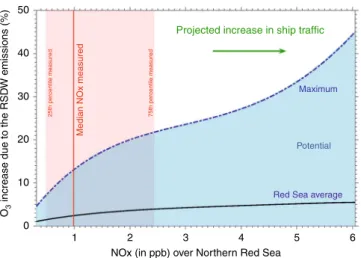
In the coming decades, ship traffic through the Red Sea and

Suez Canal is projected to increase strongly

55

, with a concomitant

rise in NO

x

emissions. From the increase of NO

x

emissions in the

model (comparing with and without the RSDW emissions) it is

expected that the degassing hydrocarbons will amplify ozone

formation in the future (Fig.

5

). The photochemical pollution

from anthropogenic NO

x

and degassing NMHCs from RSDW

will directly affect air quality, for example in Neom city, a

cross-border megaproject in the Tabuk Province of north-western

Saudi Arabia

56

_.

Methods

The AQABA ship campaign. To study the Air Quality and climate in the Ara-bian Basin (AQABA), a ship expedition was conducted in July and August 2017. The research vessel Kommandor Iona (IMO: 8401999,flag: UK, length overall × breadth extreme: 72.55 m × 14.9 m) was equipped withfive air-conditioned laboratory containers that hosted a large suite of atmospheric gas and aerosol measurement equipment. The ship sailed from Toulon (France), crossed the Mediterranean Sea, and through the Suez Canal covered the periphery of the Arabian Peninsula to Kuwait and back. In total, 20,000 km of the marine route was covered with an average speed of 3.4 ± 1.8 m s−1over the course of 60 days. Further information on the AQABA ship campaign can be found elsewhere in the literature16,17,57_.

Non-methane hydrocarbon measurements. Non-methane hydrocarbons (C2–C8) were measured in situ with two coupled, commercial gas

chromatography-flame ionization detectors (GC-FID; AMA Instruments GmbH, Germany). Detailed information on the instrumentation, experimental setup, sampling, and calibrations can be found elsewhere16_{. Briefly, atmospheric samples}

were collected through a common 5.5-m tall (3 m above the container), 0.2-m-diameter, high-flow (≈10 m3_min−1_{) stack with a subflow of 2.5 L m}−1_{. The air} passed through a PTFEfilter (5-μm pore size, Sartorius Corporate Administration GmbH, Germany) and heated (40 °C) Teflon lines before it was drawn into the instruments with aflow of 90 sccm (2 × 45 cm3_{(stp) min}−1_{(sccm)). An ozone} scrubber (Na2S2O3-infused quartzfilters) and a Nafion dryer (500-sccm counter-flow) were used to eliminate the effects of ozone and humidity in sample collection. The sampling times and volumes were adjusted according to ambient NMHC concentrations and wave conditions. During polluted conditions (e.g., Arabian Gulf and the Suez Canal) short sampling times (10 min) and small volumes (450 mL) allowed higher time resolution (50 min per measurement), while under clean conditions, such as those found in the Arabian Sea, longer sampling times and volumes (30 min, 1350 mL, time resolution= 1 h) improved detection limits. For most of the route, the sampling time was 20 min, the sampling volume 900 mL, and the time resolution 50 min per measurement. The diverse conditions met during the campaign led to the geographical demarcation that was used during data analysis (Supplementary Fig. 1).

Model simulations. In this work the EMAC (ECHAM5/MESSy Atmospheric Chemistry) model has been used. The EMAC model is a numerical chemistry and climate simulation system that includes submodels describing tropospheric and middle atmosphere processes and their interaction with oceans, land, and human effects18_{. It uses the second version of the Modular Earth Submodel System}

(MESSy2)4_{to link multi-institutional computer codes. The core atmospheric model}

is thefifth-generation European Centre Hamburg general circulation model (ECHAM5)19,58_{. For this study, we applied EMAC (ECHAM5 version 5.3.02, MESSy}

version 2.53.0) in the T106L31 resolution, i.e., with a spherical truncation of T106 (corresponding to a quadratic Gaussian grid of ~1.1 by 1.1° in latitude and longitude) with 31 vertical hybrid pressure levels up to 10 hPa. The simulations cover the period of the AQABAfield campaign, i.e., from June to September 2017. The dynamics were weakly nudged by Newtonian relaxation toward ERA-Interim reanalysis data59_{. The}

model configuration of the chemical mechanism is similar to that of Lelieveld et al.60_,

where the comprehensive MOM (Mainz Organic Mechanism)61_{NMHC chemistry}

representation has been used. Biomass-burning and anthropogenic emissions were prescribed based on the globalfire assimilation system62_{and EDGAR, v4.3.2}20,21

database, respectively. Furthermore, the emissions of ethane were subdivided into different source sectors as shown in Supplementary Figs. 2, 5, and 6. The ethane, propane, n-butanes, and i-butane emissions were scaled by factors of 1.9, 1.7, 1.0, and 0.43, respectively, to match recent global emission estimates in the literature4,15_.

Geothermal sources in the region14_{were estimated by scaling sulfuric volcanic}

emissions to 0.2 Tg yr−1. All emissions were vertically distributed following the literature58_{. Gasflares were estimated based on the work of Caseiro et al.}63_.

Positive matrix factorization. PMF is a receptor model that uses an advanced multivariate factor analysis technique that is based on weighted least-squarefits using realistic error estimates to weight data values, and by imposing non-negativity constraints in the factor computational process. PMF is widely used to identify and quantify the main sources of atmospheric pollutants64–66_{. The}

mathe-matical background of PMF analysis is comprehensively described elsewhere67_{. Briefly,}

the statistical method uses a mass balance equation, which in the receptor model is expressed as

Xij¼ Xp k¼1

GikFkjþ Eij; ð1Þ

Here, Xijis the concentration of j species measured in sample i and Gikis the species contribution of the k source to sample i. Fkj(frequently reported as source profiles) is the fraction of j species from the k source, while Eijis a residual associated with the j species concentration measured in the i sample. Finally, p denotes the total number of the sources. The goal of the model is to reproduce xijmatrix byfinding values for Gikand Fkjmatrices for a given p. The values of Gikand Fkjmatrices are adjusted until a minimum Q (the loss function) 50

40

O3

increase due to the RSD

W emissions (%) 30 20 10 0 1 2 3

NOx (in ppb) over Northern Red Sea

4 5

Red Sea average

Maximum

Projected increase in ship traffic

Median NOx measured

75th percentile measured

25th percentile measured

Potential

6

Fig. 5 Projected implications on O3formation. Increase in O3abundance over the Northern Red Sea due to the Red Sea Deep Water (RSDW) emissions.a Series of ambient NOxmixing ratios was simulated with the EMAC model by modifying the NOxemissions due to shipping. The red line indicates the median NOxmixing ratios over the Northern Red Sea for both legs. Note that over the northern Red Sea the campaign average of NOx ±s.d. mixing ratio was measured to be 2.75 ± 6.29 ppb.

for a given p is found68_{. PMF solves the receptor modeling problem by}

minimizing the loss function Q based on the uncertainty of each observation by the following equation:

Q¼X n i¼1 Xm j¼1 eij σij !2 ; ð2Þ

whereσijis an estimate of the uncertainty for the jth species in the i sample, n is the number of samples, and m is the number of species.

PMF application to volatile organic compound (VOC) source apportionment and profile contribution has been applied to a wide range of environments including urban and rural areas69–72_{. A main advantage of PMF is that it can}

provide the source profile and contribution without any prior knowledge of VOC emission profiles. In this study, PMF was applied to the 50-min data samples of the AQABA campaign for identification and quantification of the major observed VOC sources, using the US EPA PMF 5.0 software22_{(https://www.epa.gov/air-research).}

Missing points were replaced with the median concentration of the corresponding species over the entire measurement matrix and they were accompanied by an uncertainty of 4 times the species-specific median, as suggested22_{. It should be}

mentioned here that this is thefirst application of PMF to data from a moving platform (ship). This might introduce a small bias, despite the fact that the data werefiltered for own ship exhaust. It should also be noted that the background was not removed from the measurements, since the background changes as the ship travels.

Since PMF is a weighted least-squares method, individual estimates of the uncertainty in each data value are necessary. The uncertainty input data matrix followed established approaches22,73_{by including the measurement uncertainty}

of each sample and NMHC species16_{. As a complementary criterion, a}

signal-to-noise condition was additionally applied in the data as suggested in the literature72_{. Individual species that retained a significant signal were separated}

from those dominated by noise. When signal-to-noise (S/N) ratio was <0.2, species were judged as bad and removed from the analysis. Species with 0.2 < S/ N < 2 were characterized as weak and their uncertainty was tripled. Species with S/N ratio greater than 2 (S/N > 2) were defined as strong and remained unchanged.

As PMF is a descriptive model, there are no objective standards for choosing the right number of factors66_{. However, in order to acquire realistic source}

profiles and an optimum number of factors, a multicriterion was applied. This included the symmetric distribution of scaled residuals (±3σ), the investigation of all Q values (Qtrue, Qrobust, and Qexpected) (see Eq. (2)), and the interrelationship investigations between the predicted and observed volume mixing ratios. Monitoring of Q/Qexpindex with increasing number of factors was used to identify the optimal mathematical solution. The Q value is an assessment of how well the modelfits the input data. The difference between the modeled Q value and the theoretical Q value gives a good indication of the suitability of the chosen number of factors. A large decrease in the ratio is indicative of increased explanatory power in the model of the data, while a small decrease is suggestive of little improvement with extra factors. As a consequence, in most areas the number of factors was chosen after Q/Qexpindex decreased significantly (Supplementary Fig. 16). In the PMF analysis, the Q/Qexpvalues represented the ratios between the actual sum of the squares of the scaled residuals (Q) obtained from the PMF least-squaresfit and the ideal Q (Qexp), which was obtained if the fit residuals at each point were equal to the noise specified for each data point. The optimum solution suggested by the Q/Qexpratio is 4–5 factors, depending on the region of application; however, when the 5-factor solution was examined, a split in the factor was observed. Thus a 4-factor solution was selected. It has to be noted that factor 2 (Fig.1) NMHC signature remained relatively unchanged under both 4- and 5-factor outputs. Nine different modeling conditions were examined with p values (number of factors) ranging from 2 to 10 where each simulation was randomly conducted 20 times.

To evaluate the reproducibility of the PMF solution and the adequate number of PMF factors with specific focus on the original submatrix F, the bootstrap technique was applied22,73,74_{. A bootstrap data set was constructed by sampling}

blocks of observations from the original data set in random order until reaching the size of the original input data. A base bootstrap model method was carried out, executing 100 iterations, using a random seed and a minimum Pearson correlation coefficient (R value) of 0.6 as suggested in the literature69,73_{. All the}

modeled factors were well reproduced over at least 85% of runs, indicating that the model uncertainties can be interpreted, and that the number of factors is appropriate. The remaining 15% was distributed among the existing factors, while it should be noted that no runs were unmapped (unmapped is considered a factor when the bootstrap factor is not correlated to any of the base factors). For all the factors, 90% of the species (of the base run) were within the interquartile range (25th–75th percentile) of the bootstrap runs, hence highlighting the robustness of the PMF. The correlation between total VOC-reconstructed concentrations from all four factors with total VOC-observed concentrations is depicted in Supplementary Fig. 19. R2_{was 0.92, indicating good agreement} between the receptor model and the observations (Supplementary Fig. 18). This also highlights that PMF model explained almost all variance of the total concentration of the 18 VOCs.

Data availability

The data are available upon request to all scientists agreeing to the AQABA protocol (https://doi.org/10.5281/zenodo.3050041).

Received: 24 September 2019; Accepted: 2 January 2020;

References

1. Khatib, H. Oil and natural gas prospects: Middle East and North Africa. Energy Policy 64, 71–77 (2014).

2. Alvarez, R. A. et al. Assessment of methane emissions from the U.S. oil and gas supply chain. Science 361, 186–188 (2018).

3. Helmig, D. et al. Reversal of global atmospheric ethane and propane trends largely due to US oil and natural gas production. Nat. Geosci. 9, 490 (2016). 4. Pozzer, A. et al. Observed and simulated global distribution and budget of

atmospheric C2- C5alkanes. Atmos. Chem. Phys. 10, 4403–4422 (2010). 5. Hodnebrog, Ø., Dalsøren, S. B. & Myhre, G. Lifetimes, direct and indirect

radiative forcing, and global warming potentials of ethane (C2H6), propane (C3H8), and butane (C4H10). Atmos. Sci. Lett. 19, e804 (2018).

6. Haagen-Smit, A. J. Chemistry and physiology of Los Angeles Smog. Ind. Eng. Chem. 44, 1342–1346 (1952).

7. Edwards, P. M. et al. High winter ozone pollution from carbonyl photolysis in an oil and gas basin. Nature 514, 351 (2014).

8. Vickers, C. E., Gershenzon, J., Lerdau, M. T. & Loreto, F. A unified mechanism of action for volatile isoprenoids in plant abiotic stress. Nat. Chem. Biol. 5, 283–291 (2009).

9. Taylor, O. C. Importance of peroxyacetyl nitrate (PAN) as a phytotoxic air pollutant. J. Air Poll. Contr. Assoc. 19, 347–351 (1969).

10. Bourtsoukidis, E. et al. Ozone stress as a driving force of sesquiterpene emissions: a suggested parameterisation. Biogeosciences 9, 4337–4352 (2012). 11. Lelieveld, J., Evans, J. S., Fnais, M., Giannadaki, D. & Pozzer, A. The

contribution of outdoor air pollution sources to premature mortality on a global scale. Nature 525, 367 (2015).

12. Lelieveld, J. et al. Severe ozone air pollution in the Persian Gulf region. Atmos. Chem. Phys. 9, 1393–1406 (2009).

13. Aydin, M. et al. Recent decreases in fossil-fuel emissions of ethane and methane derived fromfirn air. Nature 476, 198 (2011).

14. Etiope, G. & Ciccioli, P. Earth’s degassing: a missing ethane and propane source. Science 323, 478–478 (2009).

15. Dalsøren, S. B. et al. Discrepancy between simulated and observed ethane and propane levels explained by underestimated fossil emissions. Nat. Geosci. 11, 178–184 (2018).

16. Bourtsoukidis, E. et al. Non-methane hydrocarbon (C2–C8) sources and sinks around the Arabian Peninsula. Atmos. Chem. Phys. 19, 7209–7232 (2019). 17. Pfannerstill, E. Y. et al. Shipborne measurements of total OH reactivity around

the Arabian Peninsula and its role in ozone chemistry. Atmos. Chem. Phys. 2019, 11501–11523 (2019).

18. Jöckel, P. et al. Development cycle 2 of the Modular Earth Submodel System (MESSy2). Geosci. Model Dev. 3, 717–752 (2010).

19. Roeckner, E. et al. Sensitivity of simulated climate to horizontal and vertical resolution in the ECHAM5 atmosphere model. J. Clim. 19, 3771–3791 (2006). 20. Janssens-Maenhout, G. et al. Fossil CO2 & GHG emissions of all world

countries, Vol. 107877, Luxembourg: Publications Office of the European Union, EUR 28766 EN, Publications Office of the European Union, Luxembourg, 2017, ISBN 978-92-79-73207-2,https://doi.org/10.2760/709792 (2017).

21. Crippa, M. et al. Gridded emissions of air pollutants for the period 1970–2012 within EDGAR v4. 3.2. Earth Syst. Sci. Data 10, 1987–2013 (2018). 22. Norris, G., Duvall, R., Brown, S. & Bai, S. Epa positive matrix factorization

(PMF) 5.0 fundamentals and user guide prepared for the US environmental protection agency office of research and development, Washington, DC, Inc., Petaluma (2014).

23. Holzinger, R. et al. Biomass burning as a source of formaldehyde, acetaldehyde, methanol, acetone, acetonitrile, and hydrogen cyanide. Geophys. Res. Lett. 26, 1161–1164 (1999).

24. Broadgate, W. J., Liss, P. S. & Penkett, S. A. Seasonal emissions of isoprene and other reactive hydrocarbon gases from the ocean. Geophys. Res. Lett. 24, 2675–2678 (1997).

25. Ratte, M., Plass‐Dülmer, C., Koppmann, R., Rudolph, J. & Denga, J. Production mechanism of C2‐C4 hydrocarbons in seawater: field

measurements and experiments. Glob. Biogeochem. Cycles 7, 369–378 (1993). 26. Plass‐Dülmer, C., Koppmann, R., Ratte, M. & Rudolph, J. Light nonmethane

hydrocarbons in seawater. Glob. Biogeochem. Cycles 9, 79–100 (1995). 27. Wanninkhof, R. Relationship between wind speed and gas exchange over the

28. Wanninkhof, R. & McGillis, W. R. A cubic relationship between air-sea CO2 exchange and wind speed. Geophys. Res. Lett. 26, 1889–1892 (1999). 29. Ehrhardt, A. & Hübscher, C. The Red Sea 99–121. (Springer, Berlin,

Heidelberg, 2015).https://doi.org/10.1007/978-3-662-45201-1.

30. Pautot, G., Guennoc, P., Coutelle, A. & Lyberis, N. Discovery of a large brine deep in the northern Red Sea. Nature 310, 133–136 (1984).

31. Schmidt, M., Al-Farawati, R. & Botz, R. The Red Sea. (Springer, Berlin, Heidelberg, 2015).https://doi.org/10.1007/978-3-662-45201-1.

32. Yao, F. & Hoteit, I. Rapid Red Sea Deep Water renewals caused by volcanic eruptions and the North Atlantic Oscillation. Sci. Adv. 4, eaar5637 (2018). 33. Jean-Baptiste et al. Red Sea deep water circulation and ventilation rate

deduced from the He-3 and C-14 tracerfields. J. Mar. Syst. 48, 37–50 (2004). 34. Botz, R., Schmidt, M., Wehner, H., Hufnagel, H. & Stoffers, P. Organic-rich

sediments in brine-filled Shaban-and Kebrit deeps, northern Red Sea. Chem. Geol. 244, 520–553 (2007).

35. Eder, W., Ludwig, W. & Huber, R. Novel 16S rRNA gene sequences retrieved from highly saline brine sediments of Kebrit Deep, Red Sea. Arch. Microbiol. 172, 213–218 (1999).

36. Eder, W., Jahnke, L. L., Schmidt, M. & Huber, R. Microbial diversity of the brine-seawater interface of the Kebrit Deep, Red Sea, studied via 16S rRNA gene sequences and cultivation methods. Appl. Environ. Microbiol. 67, 3077–3085 (2001).

37. Ostapoff, F. Hot Brines and Recent Heavy Metal Deposits in the Red Sea: A Geochemical and Geophysical Account, 18–21. (Springer-Verlag, Berlin, Heidelberg, 1969)https://doi.org/10.1007/978-3-662-28603-6(ISBN 978-3-662-28603-6).

38. Backer, H. & Schoell, M. New deeps with brines and metalliferous sediments in the Red Sea. Nat. Phys. Sci. 240, 153–158 (1972).

39. Bonatti, E. et al. Geophysical, geological and oceanographic surveys in the Northern Red Sea. ISMAR Bologna Techn. Rep. 94, 1–40 (2005). 40. Schmidt, M. et al. High-resolution methane profiles across anoxic

brine–seawater boundaries in the Atlantis-II, Discovery, and Kebrit Deeps (Red Sea). Chem. Geol. 200, 359–375 (2003).

41. Yao, F. et al. Seasonal overturning circulation in the Red Sea: 1. Model validation and summer circulation. J. Geophys. Res. 119, 2238–2262 (2014). 42. Osipov, S. & Stenchikov, G. Regional effects of the Mount Pinatubo eruption

on the Middle East and the Red Sea. J. Geophys. Res. 122, 8894–8912 (2017). 43. Osipov, S. & Stenchikov, G. Simulating the regional impact of dust on the

Middle East climate and the Red Sea. J. Geophys. Res. 123, 1032–1047 (2018). 44. Genin, A., Lazar, B. & Brenner, S. Vertical mixing and coral death in the Red Sea following the eruption of Mount Pinatubo. Nature 377, 507–510 (1995). 45. Woelk, S. & Quadfasel, D. Renewal of deep water in the Red Sea during

1982–1987. J. Geophys. Res. 101(C8), 18155–18165 (1996).

46. Zhan, P., Krokos, G., Guo, D. & Hoteit, I. Three-dimensional signature of the Red Sea eddies and eddy-induced transport. Geophys. Res. Lett. 46, 2167–2177 (2019).

47. Aleynik et al. Impact of remotely generated eddies on plume dispersion at abyssal mining sites in the Pacific. Sci. Rep. 7, 16959 (2017).

48. Al-Ahmadi, Khalid, Al-Amri, Abdullah & See, Linda A spatial statistical analysis of the occurrence of earthquakes along the Red Seafloor spreading: clusters of seismicity. Arab. J. Geosci. 7, 2893–2904 (2014).

49. Valentine et al. Propane respiration jump-starts microbial response to a deep oil spill. Science 330, 208–211 (2010).

50. Antunes, A., Ngugi, D. K. & Stingl, U. Microbiology of the Red Sea (and other) deep‐sea anoxic brine lakes. Environ. Microbiol. Rep. 3, 416–433 (2011). 51. Kirschke, S. et al. Three decades of global methane sources and sinks. Nat.

Geosci. 6, 813 (2013).

52. Roberts, J. M. The atmospheric chemistry of organic nitrates. Atmos. Environ. 24, 243–287 (1990).

53. Lee, J.-B. et al. Peroxyacetyl nitrate (PAN) in the urban atmosphere. Chemosphere 93, 1796–1803 (2013).

54. Monks, S. A. et al. Using an inverse model to reconcile differences in simulated and observed global ethane concentrations and trends between 2008 and 2014. J. Geophys. Res. 123, 11–262 (2018).

55. Deidun, A. et al. Assessing the potential of Suez Canal shipping traffic as an invasion pathway for non-indigenous species in central Mediterranean harbours. Rapp. Comm. Int. Mer. Méditerranée 41, 429 (2016).

56. Attia, S., Shafik, Z., & Ibrahim, A. New Cities and Community Extensions in Egypt and the Middle East: Visions and Challenges, 35–49 (Springer International Publishing)https://doi.org/10.1007/978-3-319-77875-4(2019). 57. Eger, P. G. et al. Shipborne measurements of ClNO2in the Mediterranean Sea

and around the Arabian Peninsula during summer. Atmos. Chem. Phys. 19, 12121–12140 (2019).

58. Pozzer, A. et al. Distributions and regional budgets of aerosols and their precursors simulated with the EMAC chemistry-climate model. Atmos. Chem. Phys. 12, 961–987 (2012).

59. Dee, D. P. et al. The ERA-Interim reanalysis: configuration and performance of the data assimilation system. Quart. J. R. Meteor. Soc. 137, 553–597 (2011).

60. Lelieveld, J., Gromov, S., Pozzer, A. & Taraborrelli, D. Global tropospheric hydroxyl distribution, budget and reactivity. Atmos. Chem. Phys. 16, 12477–12493 (2016).

61. Sander, R. et al. The community atmospheric chemistry box model CAABA/ MECCA-4.0. Geosci. Model Dev. 12, 1365–1385 (2019).

62. Kaiser, J. et al. Biomass burning emissions estimated with a globalfire assimilation system based on observedfire radiative power. Biogeosciences 9, 527–554 (2012).

63. Caseiro, A., Gehrke, B., Rücker, G., Leimbach, D. & Kaiser, J. W. Gasflaring activity and black carbon emissions in 2017 derived from Sentinel-3A SLSTR. Earth Syst. Sci. Data Discuss.https://doi.org/10.5194/essd-2019-99(2019). 64. Bari, M. A., Kindzierski, W. B., Wheeler, A. J., Héroux, M.-È. & Wallace, L. A.

Source apportionment of indoor and outdoor volatile organic compounds at homes in Edmonton, Canada. Build Environ. 90, 114–124 (2015). 65. Crippa, M. et al. Organic aerosol components derived from 25 AMS data sets

across Europe using a consistent ME-2 based source apportionment approach. Atmos. Chem. Phys. 14, 6159–6176 (2014).

66. Belis, C., Larsen, B. & Amato, F. European guide on with receptor models air pollution source apportionment. JRC Ref. Rep.https://ec.europa.eu/jrc/en/ publication/reference-reports/european-guide-air-pollution-source-apportionment-receptor-models(2013).

67. Paatero, P. & Tapper, U. Positive matrix factorization: a non-negative factor model with optimal utilization of error estimates of data values.

Environmetrics 5, 111–126 (1994).

68. Paatero, P., Hopke, P. K., Song, X.-H. & Ramadan, Z. Understanding and controlling rotations in factor analytic models. Chemometr. Intell. Lab. Syst. 60, 253–264 (2002).

69. Brown, S. G., Frankel, A. & Hafner, H. R. Source apportionment of VOCs in the Los Angeles area using positive matrix factorization. Atmos. Environ. 41, 227–237 (2007).

70. Morino, Y., Ohara, T., Yokouchi, Y. & Ooki, A. Comprehensive source apportionment of volatile organic compounds using observational data, two receptor models, and an emission inventory in Tokyo metropolitan area. J. Geophys. Res. 116,https://doi.org/10.1029/2010jd014762(2011).

71. Baudic, A. et al. Seasonal variability and source apportionment of volatile organic compounds (VOCs) in the Paris megacity (France). Atmos. Chem. Phys. 16, 11961–11989 (2016).

72. Leuchner, M. et al. Can positive matrix factorization help to understand patterns of organic trace gases at the continental Global Atmosphere Watch site Hohenpeissenberg? Atmos. Chem. Phys. 15, 1221–1236 (2015). 73. Polissar, A. V., Hopke, P. K., Paatero, P., Malm, W. C. & Sisler, J. F.

Atmospheric aerosol over Alaska: 2. Elemental composition and sources. J. Geophys. Res. 103, 19045–19057 (1998).

74. Paatero, P., Eberly, S., Brown, S. G. & Norris, G. A. Methods for estimating uncertainty in factor analytic solutions. Atmos. Meas. Tech. 7, 781–797 (2014).

Acknowledgements

We acknowledge the fruitful collaborations with the Cyprus Institute (CyI), the King Abdullah University of Science and Technology (KAUST), and the Kuwait Institute for Scientific Research (KISR). We are grateful to Hays Ships Ltd, the ship’s captain Pavel Kirzner, and the ship crew for providing the best possible working conditions onboard Kommandor Iona. We thank all the participants of the AQABA ship campaign and in particular Hartwig Harder for the fruitful discussions and day-to-day organization of the campaign, and Marcel Dorf, Claus Koeppel, Thomas Klüpfel, and Rolf Hofmann for logistics organization and assistance during the setup phase. Uwe Parchatka is acknowledged for his contribution to the NOxdata set. Marc Delmotte, Laurence

Vialettes, and Olivier Laurent are acknowledged for helping with setting up the methane measurements. NW acknowledges funding by the European Union’s Horizon 2020 research and innovation program under the Marie Skłodowska-Curie grant agreement No. 674911. We acknowledge the EMME-CARE project from the European Union’s Horizon 2020 Research and Innovation Programme (grant agreement No. 856612), as well as matching co-funding by the Government of the Republic of Cyprus.

Author contributions

E.B. performed the NMHC measurements, analyzed the data, and drafted the article. A.P. conducted the model simulations. T.S. investigated the potential RSDW sources. VM performed the PMF analysis. L.E. performed the NMHC measurements during the second leg. A.E., C.S., E.P. and N.W. provided the PTR–ToF–MS data, I.T. and H.F. the NOxdata, and J.D.P. the methane concentrations. D.W. and T.K. analyzed the back

trajectories. S.O. investigated the circulation in the Red Sea. J.L. conceived and directed the overall project. J.W. supervised the measurements and interpretation. All authors contributed to editing the article.

Competing interests

The authors declare no competing interests.

Additional information

Supplementary information is available for this paper at https://doi.org/10.1038/s41467-020-14375-0.

Correspondence and requests for materials should be addressed to E.B.

Peer review information Nature Communications thanks Mark Schmidt and other, anonymous, reviewer(s) for their contributions to the peer review of this work. Peer review reports are available.

Reprints and permission information is available athttp://www.nature.com/reprints

Publisher’s note Springer Nature remains neutral with regard to jurisdictional claims in published maps and institutional affiliations.

Open Access This article is licensed under a Creative Commons Attribution 4.0 International License, which permits use, sharing, adaptation, distribution and reproduction in any medium or format, as long as you give appropriate credit to the original author(s) and the source, provide a link to the Creative Commons license, and indicate if changes were made. The images or other third party material in this article are included in the article’s Creative Commons license, unless indicated otherwise in a credit line to the material. If material is not included in the article’s Creative Commons license and your intended use is not permitted by statutory regulation or exceeds the permitted use, you will need to obtain permission directly from the copyright holder. To view a copy of this license, visithttp://creativecommons.org/ licenses/by/4.0/.