Deep embedding approach to classify purpose of trips between cities from GPS data

Deep Embedding Approach to Classify Purpose of

Trips between Cities from GPS Data

by

May Alhazzani

Submitted to the Program in Media Arts and Sciences, School of

Architecture and Planning

in partial fulfillment of the requirements for the degree of

Master of Science in Media Arts and Sciences

at the

MASSACHUSETTS INSTITUTE OF TECHNOLOGY

September 2019

®Massachusetts

Institute of Technology 2019. All rights reserved.

Signature redacted

Author ...

Program in Media Arts and Sciences, School of Architecture and

Planning

Signature redacted'

August 9, 2019

Certified by...

/0

Professor Iyad Rahwan

Associate Profe or of Media Arts and Sciences

Massachusetts Institute of Technology

Accepted by ...

MASSACHUS:LNGSTITUTE OF TECHNOLOGY

OCT

0 4

2019

Thesis Supervisor

Signature redacted

.

..

...

. . . -

...

('rofessor Tod Machover

Academic Head, Program in Media Arts and Sciences

Deep Embedding Approach to Classify Purpose of Trips

between Cities from GPS Data

by

May Alhazzani

Submitted to the Program in Media Arts and Sciences, School of Architecture and Planning

on August 9, 2019, in partial fulfillment of the requirements for the degree of

Master of Science in Media Arts and Sciences

Abstract

I present a computational framework to identify purpose of trips between cities from

GPS traces using a deep embedding approach. I extracted statistical features that

captures trips characteristics that includes: temporal features, spatial features and Points of Interests (POI) features. I deployed a deep learning model to extract repre-sentative features in a lower dimensional space, which I then feed to a classic clustering algorithm to uncover purpose of trips. I detected six main purposes from trips coming from five different metropolitan areas in the United States to New York city. The trips' purposes detected are: work, which is the most dominating in size, entertain-ment, shopping, academic, and travelling. I interpret and discuss each cluster in terms of its features. I also compare cities from which trips originated by the distribution of their trips purposes.

Thesis Supervisor: Professor Iyad Rahwan

Title: Associate Professor of Media Arts and Sciences Massachusetts Institute of Technology

Deep Embedding Approach to Classify Purpose of Trips between Cities

from GPS Data

by

May Ahazzani

This thesis has been reviewed and approved by the following committee

members:

Signature redacted,

Professor Alex Pentland...

... ... ...Z-...,....

Professor of Mediar

and Sciences

Massachusetts Institute of Technology

Signature redacted

Professor Esteban Moro Egido ....

Visiting Prof sor of Media Arts and Sciences

Massachusetts Institute of Technology

Acknowledgments

I would like to thank my advisor Iyad Rahwan for giving me the freedom to explore my research interests and conduct this research. I would also like to thank my thesis reader Esteban Moro for advising me throughout this project. I want to express my gratitude for being part of the Media Lab community, where I met amazing colleagues. I am mostly grateful for my wonderful husband Thamer who has been incredibly supportive throughout my journey.

Contents

1 Introduction 1.1 M otivation . . . . 1.2 Contribution . . . . 1.3 Framework . . . . 1.4 Structure ... 2 Literature Review 2.1 Datasets . ... . 2.2 Applications of Human Mobility .

2.3 Methods of Human Mobility . . .

2.4 Trips Purposes Classification . . .

3 Data Description, Preparation, 3.1 GPS Traces . . . . 3.2 Trips Extractions . . . . 3.3 Points of Interests . . . . 3.4 Assigning Trips to POIs . . .

3.5 General Statistics . . . . 3.6 Cleaning . . . . 4 Features Extraction 4.1 Temporal features . . . . 4.1.1 Duration . . . . 11 11 11 12 14 15 . . . 15 . . . 16 . . . 17 . . . 18 and Enrichment . . . . . . . . . . . . 20 . . . . 20 . . . . 21 . . . . 23 . . . . 23 . . . . 26 . . . . 32 34 35 35 ... ...

4.1.2 HourlyActivities . . . . 35 4.1.3 WeeklyActivities . . . . 36 4.2 PointsofInterestsFeatures. . . . . 38 4.3 RadiusofGyration . . . . 39 4.4 EntropyofPOIsTypes . . . . 41 5 Methods 43 5.1 Dimensionality Reduction . . . . 43 5.2 Deep Embedding . . . . 43 5.2.1 Model . . . . 44 5.2.2 Training . . . . 45 5.3 Classification . . . . 45

6 Results and Interpretations 49 6.1 Purpose of Trips Clusters . . . . 49

6.2 Cities Comparisions . . . . 53

6.3 Trips' Purposes and Applications . . . . 60

7 Conclusion and Future Work 62 7.1 Conclusion . . . . 62

List of Figures

1-1 Framework of detecting purpose of trips from Global Positioning Sys-tem (GPS) and Points of Interests (POIs) data. Highlited are the four main steps of the framework . . . . 13

3-1 Example of center of stay(red) found from aggregating mulitple points

(blue) that are close in space and time . . . . 22

3-2 The distribution of the number of stays per trip. A distribution with

a long tail is detected, which matches distributions of number of tra-jectories per trip from other mobility sources studied in the literature 22

3-3 Most popular POI types in New York area . . . . 24

3-4 Points of Interests (POIs) density distribution in New York area . . . 25

3-5 Example of a stay point in a dense POIs location. The visitor can be

staying at any of the POIs within the labeled radius. . . . . 26 3-6 The number of unique users who traveled between cities. Some flows

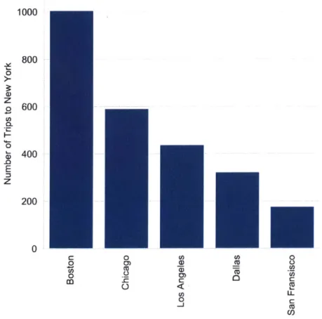
are high due to the close proximities between the source and destination cities, or perhaps due to other reasons. . . . . 28 3-7 The number of trips to New York area from different cities . . . . 29

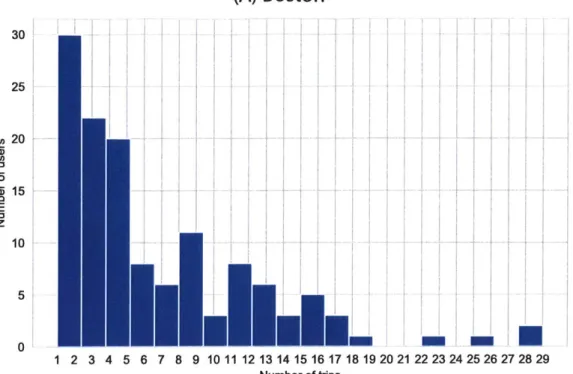
3-8 The number of trips per user (recurrent trips that the same users make)

for visitors to New York area that come from (a) Boston and (b) Los A ngeles. . . . . 30 3-9 The number of stays per trip of travelers from Boston to New York area 31 3-10 Hatmaps showing the density of stays in New York area from visits

3-11 The valid and outlier trips according to the duration (in days) and

the number of trajectories. Trips beyond 30 days of duration, and less than 4 trajectories are considered outliers. . . . . 33

4-1 The distirbution of duration of trips in days, showing that the majority of trips are below 5 days . . . . 36

4-2 Examples of different visits' activities hourly. This shows that different trips have different behaviors of activities hourly. . . . . 37

4-3 Examples of different visits activities over days of the week. This shows that different trips have different behaviors of activities over days of the w eek. . . . . 38

4-4 POI types with highest (top) and lowest (bottom) IDF scores. Notice that popular POI types have low IDF scores and rare POIs have high ID F scores. . . . . 40 4-5 The distribution of radius of gyration calculated in Kilometers. .... 41 4-6 The distribution of entropy in POI types visited . . . . 42

5-1 The general structure of an autoencoder. It consists of two main parts:

the encoder, which encodes the input to embedded features, and the decoder, which reconstructs the original input from the embedded fea-tures . . . . 45

5-2 The learning curve of training the autoencoder . . . . . ... . . . . 46

5-3 Mean Sum of Square Error (SSE) for multiple K values for K-means on embedded features of trips . . . . 48

6-1 The number of trips in each cluster of trips' purposes. This shows that Work is the dominating purpose of travel between cities . . . . 53 6-2 Points of Interests (POI) types that are most significant for each cluster

found ordered by their TFIDF scores. This highlights the type of activities in which users engaged for each cluster of purpose of trips found . . . . 54

6-3 The density of destinations visited of trips in each cluster . . . . 55

6-4 Features of identified purpose of trips. Showing the mean of (A) Du-ration in days (B) Entropy of POI types , and (C) Radius of gyration in K ilom eters . . . . 56

6-5 The mean of ratio of stays over days of the week for each cluster . . . 57 6-6 The mean of ratio of stays over hours of the day for each cluster . . . 58

6-7 The distribution of trip purposes detected from each source city to New

Y ork area . . . . 59 6-8 Heatmap of destinations of trips in Manhattan, New York, for each

List of Tables

5.1 The dimensions of each feature extracted for the classification of pur-pose of trips task . . . . 44

5.2 Layers of the encoder and the demotions of the input and output of

each layer. The layers of the decoder are the same, but in reverse order 46

Chapter 1

Introduction

1.1

Motivation

Identifying the purpose of trips between regions on large scale has many useful ap-plications. One is understanding the relationships among regions, which is useful in transportation planning, placement of business and services, and understanding economical influence and dependence between regions. Another useful application of identifying purpose of trips is in urbanism and transportation. Understanding the amount and pattern of visits is valuable to cities to increase accessibility to places. Accessibility can be increased by providing infrastructures such as roads, public tran-sit systems, and autonomous cars planning. In addition, it gives important insights to urban planners on why people visit their cities and what type of attractions and actives bring visitors.

1.2

Contribution

Identifying the purpose of travel on large scale, between cities, based on digital human mobility has not been yet explored. This may be due to limitations in availability of data that captures human mobility on large scale. However, recently GPS traces and phone data allows for existence of large scale digital traces from which human mobil-ity can be captured with good qualmobil-ity and large scale. In this research, I aimed to

utilize these data sets in extracting large scale mobility between regions and identify trip purposes using a deep embedding approach.

Flights and trains datasets only provide the number of visitors through airports and train stations. It is not a sufficient source to provide other insights about the visits, like the activities visitors do once they arrive to their destinations.

1.3

Framework

I present a computational framework to process, enrich, and classify trips' data to identify purpose of trips between cities. Phone and GPS trajectory data are raw and lack the necessary semantic information, such as the activity types performed after the end of the trip. The challenge is that trajectory data is rich in sequence of coordinates, but lacks activity information that can indicate the intended purpose of mobility. Thus, I enriched the data with both trip semantics and visited venues semantics. For trip semantics, I extracted spatial and temporal features from tra-jectories. For venues semantics, I mapped trajectories to Points of Interests (POI),

which identifies the type of place the user visited.

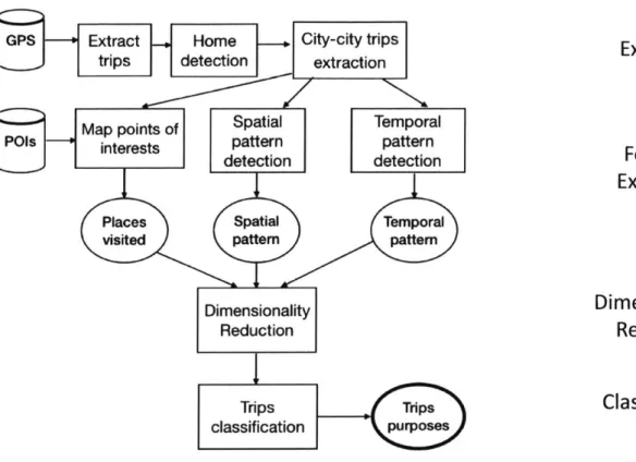
The computational framework to identify purpose of trips is shown in Figure 1-1. The framework is based on unsupervised classification methodology of deep embed-ded features. It uses two types of raw datasets : GPS traces and Points of Interests (POIs). There are four main steps to identify purpose of tips. First, in trips extrac-tion, meaningful trips are extracted between cities. Then, in the feature extraction step, statistical features are mined including spatial and temporal features of trips, in addition to POI features. Then, in the dimensionality reduction step, deep embed-ding is used to get low dimensional features. Finally, in the classification step, the embedded features are used in a clustering algorithm to identify clusters of purpose of trips.

GPS Extract - Home City-city trips trips detection extraction

Map points of Spatial Temporal

POls interests pattern pattern

inteests detection _detection

Places Spatial Temporal visited pattem pattem

Dimensionality Reduction Trips Trips classification purposes Trips Extraction Features Extraction Dimensionality Reduction Classification

Figure 1-1: Framework of detecting purpose of trips from Global Positioning System

(GPS) and Points of Interests (POIs) data. Highlited are the four main steps of the

1.4

Structure

In the following chapters, I will review previous work in the domain of human mobility in the Literature Review section. Then, in Data Description and Preparation, I show how the raw datasets are processed and discuss general statistics of the data. Then, in Features Extraction, I discuss the statistical features extracted from datasets to be used in the classification. Next, in Methods, I discuss the methods of dimensionality reduction and classification. Afterwards, in the Results and Interpretation, I discuss and interpret the clusters of purpose of trips detected. Finally, in the Conclusion and Future work, I conclude the main outcomes and provide direction of extending the work in the future.

Chapter 2

Literature Review

2.1

Datasets

There are multiple data sources that has been used to captures movement between areas. Most traditional sources are Census data and travel surveys. Census data is collected by periodical national surveys in which householders are asked about de-mographical and economical information in addition to workplace. This can be used to estimate the flow between home-work places. However, it doesn't provide precise time and location of the trips users make. Also, it is hard to keep updated as it's collected manually, which is costly

[1].

Local travel surveys are more detailed since it is focused on transportation information of users. However, they suffer from similar disadvantages. Travel surveys are also restricted by covering limited areas and small sample of the population. Moreover, it doesn't capture actual real-time trips

[17][26].

With the ubiquity of mobile phone and then smart phones that captures GPS data, new data sources are utilized to capture mobility of users. A popular source is Call Detail Records (CDRs) , that are collected for billing purposes by telecom companies. The data provides timestamps and location of connecting tower of calls and activities (e.g. messaging, and connecting to the Internet). Thus, CDRS can be used to infer human mobility. Multiple studies utilized CDRs for large scale human mobility modeling [11],[29]. A more accurate location data source is Global

Positioning System

(GPS)

traces that are collected for functionality of smart phones and other GPS navigation devices. These data sources offer dynamic, time accurate, and spatially accurate, with high granularity, data. The error range is only 10 to 15 meters radius using the best GPS satellite technology. The data is collected digitally, up to date, and cheap to collect. One public data source that was published is the GeoLife project, which was launched by Microsoft, made GPS trajectories from 182 individuals publicly available online. Many research papers utilized that data for research of human mobility inferred from GPS traces [39][41].

2.2

Applications of Human Mobility

Human mobility mined from digital traces such as mobile phone data and GPS traces has been a domain of great interest due to a variety of useful applications. Mobile phone and GPS data allows for implicit traces of when and where people move. In the literature, it has been used to develop many useful applications mainly in trans-portation and urbanism. Research papers discussed identifying pattern of human mobility to uncover laws that governs human mobility [11], in addition to under-standing road usage patterns [33]. Moreover, researchers developed models to esti-mate travel demand

[31],

and develop transportation models based on phone data to complement tradition transportation models [3]. Additionally, researchers developed methods to identify transportation mode used by users (e.g. cars, public transit, walk, or bike)[27]. Moreover, research papers discussed predicting future mobility us-ing machine learnus-ing models [23] [18] and understandus-ing limits of predictability usus-ing entropy in space and time as metric of randomness of movements [12].

Human mobility has applications in different domains. It's used to identify land use by clustering mobility activities in districts visited to identify common patterns

[32]. Also, mobility was used to detect demographical features such as age and

in-come [9]. Moreover, it has been used in other domains such as recommendation of places for businesses by mapping trips to points of interests data [38], in epidemics

to understand spread of diseases [30][34] , in extreme events detections by identifying outlier behaviors [10], and many others.

2.3

Methods of Human Mobility

From raw signals collected from phone billing data or GPS traces, many methods were developed to capture human mobility. Trajectories from mobile phones and GPS must be cleaned to eliminate points or calls made in the middle of routes (passing by points). Thus, algorithms have been developed to extract meaningful points named "stays" that are extracted from raw trajectories to eliminate noise and extract origins and destinations of trips

[31][40][16].

From raw trajectories, points close in time and space are grouped into stay points. Stay points are computes as the mean location of trajectory points within a time and distance thresholds. Typically, threshold values used are 300-500 meters radius for phone data, and 50-200 meters radius for GPS data with 5 minutes time window [16]. Using such standard stay points extraction method in human mobility pipelines, researchers showed correlated results with survey transportation data [15].

In addition to trip extraction, main activity detection such as home and work is an essential component in human mobility pipeline tasks. Typically, home is identified as the place where the user has the most, frequent activities during nights of weekdays. The exact time window of nighttime can be adjusted according to location and typical routine for the city or country (such as 7 pm to 7 am). Employing such simple approach has been shown to have significant correlation with survey data

[15].

In addition, methods were developed to capture dynamic night time per user (for users with different time schedules). A Gaussian mixture model was fitted on temporal and spatial activities of users to identify their home and work locations [8].

Augmenting raw trajectory data with information from external datasets to en-rich its value has been a popular approach. A paper [28] showed augmenting GPS traces of small number of tracked users with contextual information, like residential

location, age, or gender, helps in identifying visited places. Methods of extracting semantic features from GPS trajectories is presented in

[37],

where semantic behav-ior including geometric, and temporal features are utilized. Moreover, methods were developed to map GPS traces to interesting locations (important landmarks in the city), where researchers used hierarchical graph based method and included user's previous history in identifying visited locations. The method was applied on dataset of 107 uses over the course of one year

[41].

Furthermore, location data was enriched with demographical information from tract census dataset such as income [5].

2.4

Trips Purposes Classification

Trip purpose identification from human mobility has been of interest due to its use-fulness in many applications. A recent paper [7] used deep embedding, similar to word2vec method [24], on features from Taxi trips in New York city to identify pur-pose of trips into work, recreational, dining, and other purpur-poses. They show superior results using deep embedding against feeding raw features to the classifier. Another paper [2] used temporal features from phone data in Boston metropolitan area to identify purpose of trip into work, home, and other. They show good accuracy on ag-gregate level evaluated against transportation surveys. Another paper [25] presented trip purpose identification on small number of participants (156) in Switzerland based on their GPS traces augmented with demographic information using random forest method.

A recent paper [22] used graph convolutional neural networks to predict purpose

of trips. They used personalized graphs per user to capture habitual features, then feed it to a convolutional neural network to identify purpose of trips with labeled data. They used GPS survey data based on 139 users, where uses log their activities. Additionally, a recent paper [6] used a Bayesian framework to identify purpose of trips from taxi pickup/drop-off data in New York city. They first used spatial clustering to identify candidate activity areas, then they infer the priori probability for each

activity using spatio-temporal patterns. Moreover, a paper utilized a labeled survey

GPS data, to predict purpose of trips by a supervised machine learning method using

a neural network. The researchers utilized land use information based on polygons and point of interest to identify purpose of trips on aggregated areas [35].

Chapter 3

Data Description, Preparation, and

Enrichment

In this Chapter, I describe how to extract trips from raw GPS data. In addtiotn, I describe the process of cleaning the data to have useful trips information. Also, I describe how I enriched the GPS traces with venues data that consists of the Points of Interests (POIs).

3.1

GPS

Traces

I

utilized a large scope Global Positioning System

(GPS)

traces as a proxy for human mobility between cities. GPS is a global navigation satellite system that provides ge-olocation and time information to a GPS receiver that exist in modern mobile phones. The GPS data used are collected from mobile phone applications for general purposes that requires location such as weather prediction. It spans 6 months, and it covers multiple metropolitan areas in the US.

The raw GPS data consists of records of the coordinates and timestamps of the phone location. The number of records is typically large as it captures many points that is close in time and space. It requires processing to extract clean mobility information that is useful. Typically, GPS systems are accurate within 10-15 meters

radius [39]. The next section will describe how the raw data is processed to extract useful trips information.

3.2

Trips Extractions

In order to extract useful mobility information from raw GPS data, The following steps are applied:

•

Stay points:

First, GPS points that are close in time and space are aggregated to identify "stay points", which denote where the user was staying. A stay point is com-puted from GPS points within a radius of 15 meters and a minimum duration of 5 minutes, which are standard values used in the field to detect a stay posi-ton

[39].

The coordinates of a stay point are the ones of the center of mass of the aggregated GPS points in space as illustrated in the example in Figure

3-1. The time of stay is marked by the first timestamp record of the aggregated

points. Identifying stay points also allows for filtering points while moving, such as while walking or driving, as we aim to extract places where the user actually stopped and engaged in some activity. Figure 3-2 shows the distribution of num-ber of stays per user. Getting an exponential distribution of stays matches the distributions found in mobility from other sources such as Call Detail Records

(CDR) data [12].

* Home extraction:

Identifying home locations from mobility data such as GPS or phone records is well known task in the literature. Following the standard method, the home city for a user is identified as the place where a minimum of 25 weeknight stays is spent. Home city is extracted for users in order to identify the direction of travel.

* Trip extraction:

Points Stay center

Figure 3-1: Example of center of stay(red) found from aggregating mulitple points (blue) that are close in space and time

cc E z 140 -1 2 100 -80 -60 40 20 0K 0 20 40 60 80 100 120 140 160 180 200 220 240 260 280 300 320 340 360 380 400 420 440 460 480 500 Stays

Figure 3-2: The distribution of the number of stays per trip. A distribution with a long tail is detected, which matches distributions of number of trajectories per trip from other mobility sources studied in the literature

-

--minimum distance considered is 30 meters, which is a standard threshold to identify a meaningful trip between two stays. A trip is extracted between each consecutive stays of the user. The start of the trip is denoted by the timestamp of the first record of the stay points and the end of the trips is denoted by the last record of the destination stay.

e City-City visit identification:

Here, the task is to identify visits between two cities. For each user, all trips are extracted, then between cities trips are detected by inspecting the source and destination of stays. When the source and destinations are in different cities, a visit is detected. the start of the visit is the timestamp of the first stay point in the visited city, and the end of the visit is the timestamp of the last stay point.

3.3

Points of Interests

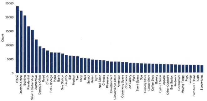
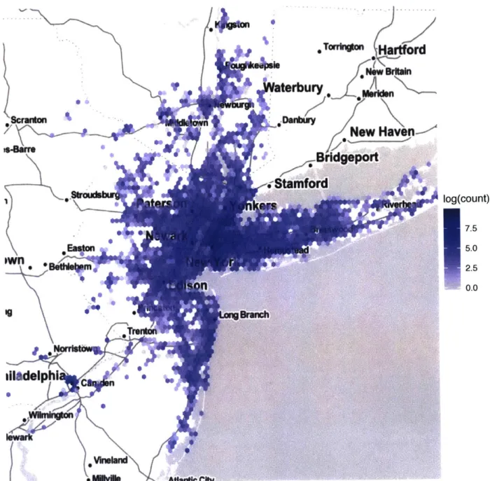
Points of Interests (POIs) identifies venues' information around cities that usually is used in maps services. I utilized Foursquare 1 venues as source of POIs around cities in the United States. The data consists of the venue's name, location as coordinates. Also, venues are classified into categories. Foursquare offers over 900 different cat-egories of venues. Additionally, it provides the number of check ins users made for each venue. The top 50 most frequent types of POIs in New York area are shown in Figure 3-3. POI data also have great spatial coverage, it is typically dense in the city center and it gets sparser as we move outside the city as shown in the map in Figure 3-4.

3.4

Assigning Trips to POIs

The goal is to enrich GPS mobility data with contextual information. The most use-ful one for the task of detecting trips purposes is to identify the types of activities in which users engaged during their travels. POIs represents an ideal source of data to

25000 20000 15000 0 10000

5000

IIIIIIIIIIIIininin

i

0

-.;c 0. fn -B C C ~ (UM D i~. i 0LD COE(LL

0 0 0 A 2 ED

E

aill

-5

05

E

Figure 3-3: Most popular POItypes in New York area

identify activities types.

The task is tomap each trip's destination to the visited POIinstance. The problem of assigning GPS trajectories to POIvenues inan unsupervised setup is challenging and is under research. This is especially challenging in POIdense areas, such as New York Manhattan

(see

Figure 3-5), where multiple POIs are present within asmall radius of the stay destination. Therefore, it ispossible that the user was visiting any of the venues within that radius. Without labeled data, where users report which place they actually visited, the problem is more challenging. Thus, we need to de-velop amethod to map trips to POIs inan unsupervised manner that captures this uncertainty.

The approach Ideveloped is to dosoft assignment of the trip's destination to possible multiple POIs. Probability assignment ofPOI1occupancy is based on two factors: the distance from the stay center and the popularity of the POIvenue. I utilized nearest neighbor algorithm (NN)1[4to identify the closest 10 POIs within 100 meter radius. Then, eachPOI1is assigned aprobability score according to equation

*4a* ISt

own,,n

tilladelphic* VkW~d ,wIeAnd *TorrkWon

Ha

rd

rbury

_AW

NewHaven--'

Br dgeport

amford log(count) 7.5

Broadway Hi-Tronics

10

Fashion Avenue

Express Trade Capital StayPoint 9

100m t P Fashion District Dental:

4-- --- -- 0- Justin Rashbaum, DMD

;Zi Fine Italian

Men'sWear

9OnDck

Capital Jordache Enterprises 9 9Chipot 4" * _&

9

DanelShoe Repair Sub.

9

Hale and Hearty

le Mexican Grill

9C Life Corporation

Figure 3-5: Example of a stay point in a dense POIs location. The visitor can be staying at any of the POIs within the labeled radius.

3.1. The algorithm of mapping trips destinations to POI instances probabilistically

is shown in the pseudocode in 3.4

pi, = wodj + wirj (3.1)

Where pi is the probability of trip i being in POI instance

j

, dij is the distance

between trip i destination and POI instance

j,

ri is the popularity of POI

j,

and

Wo

C

[0, 1] the weight of distance, and wi E [0, 1] is the weight of popularity such that

wo + Wi = 1.

3.5

General Statistics

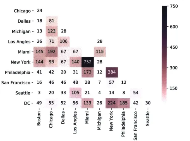
In this section, I show basic statistics of the dataset to better understand the data. The number of unique users captured traveling between cities are shown in figure 3-6. Because the stays are in continuous land, we discretize it by identifying the closest

Algorithm 1 Psudocode of mapping trips destinations to POI instances probabilis-tically based on distance and popularity weight parameters (wo,wi)

Input: POI, trips Output: probabilities

MappedPOIs,distances <- NearestNeigbor(POI,trips)

popularity <- popularity(POI)

N <- length(Mapped_POIs) for i in (0,N) do

probabilities[i] +- wO * distances[i] +wl * popularity[i]

end for

main city to the source and destination of trips. The number of trips to New York area from other cities is shown in figure 3-7. The number of trips is influenced by the number of users which correlates with population of the source city, the geographical distance, and possible other factors such as business or family relations.

It is also important to detect the recurrent trips each user makes. Some users travel periodically, while other users make few trips, and some users only visit once during the time span of the data (6 months). The number of visits per user is shown in Figure 3-8 for visitors from Boston and Los Angeles. We notice that visitors from Boston have far more recurrent trips due to the close proximities and perhaps relations that requires periodical visits.

Moreover, The amount of stays that users make in each trip is a significant statistic as it shows how much activities in which the user engaged during thier visit. The number of stays per visit is shown in Figure 3-9.

The spatial distribution of stays is an important aspect of trips statistics as well. It describes the distribution of destinations of where visitors stayed in the destina-tion city. Stays distribudestina-tion for visitors from Boston and Los Angeles are shown as heatmaps in Figure 3-10. We notice that most activities are in the city center (Man-hattan). However, in the case of Boston visitors there are stays far away from the city center. This may be due to the close distance between Boston and New York so users may have other destination to visit family or for other purposes.

Number of users 750 Chicago - 24 Dallas - 18 81 600 Michigan - 13 123 28 Los Angles - 26 71 106 28 450 Miami - 145 192 67 67 115 New York - 144 93 67 140 7 28 Philadelphia - 41 42 20 31 173 12 San Francisco - 16 46 46 48 28 7 57 12 150 Seattle - 3 20 33 105 21 4 14 8 54 DC - 49 55 52 56 133 26 224 185 42 30 r- o I C Mn 0 W3 0 ~ 0 E M U W>- 0 In EU UE

Figure 3-6: The number of unique users who traveled between cities. Some flows are high due to the close proximities between the source and destination cities, or perhaps due to other reasons.

1000 800 0 z o 600 0. 0 3 400 .o E z 200 0 8 0, a 8c F U( ti 0(

IJ

1 2 3 4 5 6 7 8 9 10

(A) Boston

30 25 20 15 10 5 0 1 2 3 4 5 6 7 8 9 10 11 Number of trips

Figure 3-8: The number of trips per user (recurrent trips that the same users make) for visitors to New York area that come from (a) Boston and (b) Los Angeles.

a) E z 0 E z 11 12 13 14 15 16 17 18 19 20 21 22 23 24 25 26 27 28 29 Number of trips

(B) Los Angeles

40 35 30 25 20 15 10 5 0

0 20 40 60 80 100 120 140 160 180 200 220 240 260 280 300 320 340 360 380 400 420 440 460 480 500

Stays

Figure 3-9: The number of stays per trip of travelers from Boston to New York area

Visitis From Boston

Ne - 1 J -wr.r wr'/ N \..~:sdsama paersd~"~Densit *Edison mladeiphia / .*Cmn

Visits From Los Angeles

NOWN

HNew

Han B, dgeport *Stamford

' rudlg Pateso nkers Rwt ad

I-Y 220

-'Edison 51

*Long~fan

vwwbm,./ ,adphAU

7"-Figure 3-10: Hatmaps showing the density of stays in New York area from visits from Boston and Los Angeles

140 120 100 0. E z 80 60 40 20 0

3.6

Cleaning

In this section, I describe removing outlier trips from data. There are trips that are disqualified to be used in classification of purpose of trips. Visits that has very long duration (beyond 30 days), are considered too long for a temporary visit. They may

indicate other types of trips such as moving to a new city or staying with family for an extended amount of time. This is beyond the scope of trips we aim to classify. Additionally, trips with no sufficient trajectory data. Lack of sufficient number of stays makes it hard to extract useful features. Thus, only trips with minimum of four or more stays are considered. Figure 3-11 shows the outlier trips and the valid trips

0 S S 0 0 0 S

- ___

__ * I * Se,~ ~~WI 0 * 0 5 6 S *.;.~.* ':~~.

::.~~*

.**.

*:i;.*

*~S*. * * ~: * q S 31*. **. ~ 0 5 5 S *~*1_____ 50 100 Stays 150 Data • noisy visits • visits 200

Figure 3-11: The valid and outlier trips according to the duration (in days) and the number of trajectories. Trips beyond 30 days of duration, and less than 4 trajectories are considered outliers.

100 C 0 0 50 0 0

Chapter 4

Features Extraction

To identify trips purposes in an unsupervised manner, it is essential to extract sta-tistical features of city-city trips that captures patterns related to different purposes of trips. In this chapter, I describe how to extract useful statistical features from the post-processed trips data as described in the previous chapter. The features are extracted from trips and stays of each city-city visit. That is when a user travels from city A to city B , we extract features on activities in which the user engaged during the entire visit. The features extracted are:

•

Temporal features:

- Duration,

- Hourly distribution of trip times

- Weekly distribution of trip times

• Points of Interests (POIs) features

" Radius of gyration

" Entropy of POIs types visited

4.1

Temporal features

The temporal aspect can reveal patterns to detect trips purposes. Temporal features of a visit consist of the time when stays (activities) take place. Temporal features include: duration of trips in days, distribution of activities over the hours of the day, and the distribution of activities over days of the week. Each feature is described in the following sections.

4.1.1

Duration

Duration represents the number of days the trip spanned. It is calculated from the time of the first stay until the last stay in the destination city as in equation 4.1. Figure 4-1 shows the distribution of trips' durations in days. We notice that most trips are within few days , that is less than 10 days. However, there are few trips that are longer. We exclude the trips beyond 30 days as they don't reflect temporary trips. These outliers may indicate moving to the destination city or extended family visits.

duration = time(stayo) - time(stayn) (4.1)

Where stayo is the first stay and stay, is the last stay in the distination city.

4.1.2

Hourly Activities

Identifying the distribution of activities over the hours of the day can help indicate the purpose of trips. Early morning activities signal work purposes while late night stays may indicate entertainment purposes. Thus, I calculated the distribution of stays over the 24 hours of the day as in equation 4.2.

En stayj C Hi

Hi = i (4.2)

r stayj

Where Hi indicate the hour i where i C [0, 23].

200 150 E100 50 0 0

0

IhEE.m.o....mu..mm

0 5 10 15 20 25 30 Duration in days

Figure 4-1: The distirbution of duration of trips in days, showing that the majority of trips are below 5 days

in the distribution of activities over the hours of the day. For instance, trip 4 shows uniform activities, where trip 1 shows activities only in the morning and in the night. This variation between trips indicate different behaviors and thus different purposes of travel.

4.1.3

Weekly Activities

Another aspect of the temporal features is indicating what days of the week in which activities take place. Typically, weekends activities are different from week-days. Weekdays activities generally indicate work related as opposed to weekends that indicate family and recreational purposes. Identifying activities distribution over weekdays can help identify purpose of trips. It is calculated as shown in equa-tion 4.3. Figure 4-3 shows five examples of trips and their distribuequa-tion of stays over days of the week.

= st, _(4.3)

02 T T rip 1 0.0 -A-N--- - - - -O.2 -

V

0.2 0.0

i

It I 0.2 t - - -

-0.2

f

I

0.0 0 .2-0 1 2 3 4 5 6 7 8 9 10 11 12 13 14 15 16 Hour

T

Trip 2

Trip

3

Trip 4 -4 Trip 5 17 18 19 20 21 22 23

Figure 4-2: Examples of different visits' activities hourly. This shows that different trips have different behaviors of activities hourly.

T 0.5 -F Trip 1 0.0 0.5 0.0 0.5 0.0 - -0.5' __-0.5 -0.0

I

-~~1 4% '9 4F

4-'9 Trip 2 Trip 3 Trip 4 Trip 5

Figure 4-3: Examples of different visits activities over days of the week. This shows that different trips have different behaviors of activities over days of the week.

Where W indicate the weekday i where i E [0, 6].

4.2

Points of Interests Features

The strongest feature that we can adopt is to identify the activities in which users engaged while visiting the destination city. Since GPS offers excellent source for high granular location data, we can utilize it and enrich it with external urban data that offers activity information. The best urban data that identifies types of places and accurate locations of venues is Points of Interests (POIs) , which was discussed in the previous chapter. Also, mapping GPS traces to POI venues is discussed in the previous chapter.

0 0

Once we have the mapped stays to POIs, we need to extract a statistic that measures activities per POI category for each trip. I used Term Frequency Inverse Document Frequency(TFIDF) metric in order to identified what POI types are visited signifi-cantly. Since some types of POIs are much more common such as office and food, it is useful to normalize the share of activities in a trip by the share of activities that all other trips have. The IDF score makes this normalization as shown in equation 4.4 . Figure 4-4 shows POI types with highest and lowest IDF scores. We see that highest scores are for the rare POI types, and the lowest scores are for the common and general ones.

n stayk E POI TF~jj)- Ek nstayk 44 N En stayk IDF- = log(

ZN

z~

kt(4.5)

z

k stayk ( POI) TFIDFij) TFj * IDF (4.6)

where TF(i,

j)

is the TF of trip i for POI type j. IDF is the IDF for POI type

j.

4.3

Radius of Gyration

Spatial features are useful to identify purpose of trips. Trips where the user's stays are mainly concentrated in few locations in close proximities is different from trips where the user's visited locations are far away from each other. The spatial spread of stays can help indicate the type of activities. Thus, I extract a statistical feature that captures the spread of stays spatially. Radius of gyration is a measure that is

wildly used in the human mobility literature [11]. It can indicate the spatial spread of

points from the center of mass. The center of mass is calculated as the mean location

of all stays of the trip. I calculate radius of gyration as in equation 4.7. Figure 4-5

shows the distribution of radius of gyration in Kilometers of trips in New York area.

POI types with highest IDF scores

Alternative Healer Christmas Market Fish & Chips

Mini Golf

-Laboratory Leather Goods Event Services Art Studio Paella Insurance Office Beer Store Religious School FrameStore Zoo Exhibit Souvenir Shop Polish Waterfall Salsa Club ATM Russian 0 2 4 6 8 10 12 OF score

POI types with lowest IDF scores

Record Shop Motel Taxi Church Professional Event Space Coworking Space Salon / Barbershop Hospital Gas Station Coffee Shop American Automotive Gym Doctor's Office Road Building Hotel Residential Office 0 2 4 6 8 10 12 IDF score

Figure 4-4: P01 types with highest (top) and lowest (bottom) IDF scores. Notice that popular P01 types have low IDF scores and rare POIs have high IDF scores.

100 80 U) 0 60 E Z 40 20 0 0 50 100 150 200 Radius of gyration (KM)

Figure 4-5: The distribution of radius of gyration calculated in Kilometers.

dj = distance(M, stay) (4.8) Where Ri is the radius of gtration of trip i. M is the mean location of all stays, and

dj is the distance of stay j to the mean.

4.4

Entropy of POIs Types

Here, I introduce a feature to measure the variety of activities a trip contained. A trip that includes many different types of activities is different form one that is focused on few types of activities such as work. Entropy is a physics concept that measures

randomness. It has been adopted in information theory to measure randomness in

information [14]. It is also well adopted in mobility literature [29]. The aim is to

measure the entropy of POI types users visited in their trips. Entropy is calculated

as in equation 4.4 . The distribution of entropy values of visits to New York is shown

in Figure 4-6. We notice the distribution is exponential, where most trips have small entropy, and fewer trips have higher entropy scores.

400 * 300 E 200 z 100 0 0.0 0.5 1.0 1.5 2.0 Entropy

Figure 4-6: The distribution of entropy in POI types visited

Si. - p log(p,?) (4.9)

where Si is the entropy of trip i, and pj is the probability assignemnt of POI type 3.

Chapter 5

Methods

5.1

Dimensionality Reduction

In the previous chapter, I showed the variety of features extracted from the data to identify purpose of trips. The dimensionality of the features extracted is large for the classification task. The features extracted and their dimensions are shown in Table

5.1. The dimensions of the POIs features are too large as we have to account of all

types of places in the city. Clustering with high dimensionality is a hard task as the concept of distance is less precise with large number of dimensions [19]. In addition, it is likely that some features are correlated, and therefore, can be reduced effectively. Thus, I reduce the dimensionality of the features by a deep embedding approach, using a'deep learning model. Then, I utilized the embedded, lower dimensional, features in a clustering algorithm to detect clusters of purposes of trips.

5.2

Deep Embedding

Deep embedding has been a popular method to reduce dimensionality in data, since the rise of deep learning models. It was shown to produce representative features that gives superior results in known classification tasks [20][36]. The state of the art method to reduce dimensionality is using Principal component analysis (PCA)

Feature Dimentions

Duration 1

Hours activities 24

Weekly activities 7

Radius of gyration 1

Points of Interests features 820

Entropy of POIs types visited 1

Total 952

Table 5.1: The dimensions of each feature extracted for the classification of purpose of trips task

embedding methods can model complex nonlinear relations that makes it effective in finding representative features. Thus, I adopted a deep embedding methodology to reduce the dimensionality and extract expressive features for the classification task.

5.2.1

Model

In this unsupervised task of classifying purpose of trips, I utilized an autoencoder model to create an embedding of features in a lower dimensional space. An au-toencoder is a neural network model, where the optimization task is to optimize the reconstruction cost from the hidden features (embedding) to the original input fea-tures. Figure 5-1 shows the general structure of an autoencoder, that contains the basic two parts. The encoder is a neural network that reduces the feature space layer after layer and produces the embedding. The decoder part is a neural network in the reverse order of the encoder, that reconstructs the original features from the embed-ded features.

The task of the autoencoder is to map the feature vector x to the reconstructed ver-sion - from the hidden (embedded) features h. The learning task is to optimize the cost function L(x,:z). The loss function measures the dissimilarity between x and using a distance functions such as the mean squared error.

To have a sparse autoencoder, the model is regularized to be sparse to respond to unique features instead of simply acting as an identity function that copies the input.

Inpu C N N -I N I ~ Embedding~ / \ - - / /

A

Ii.,, / \ I \ / - %. \ I-N Encoder Decoder

Figure 5-1: The general structure of an autoencoder. It consists of two main parts: the encoder, which encodes the input to embedded features, and the decoder, which reconstructs the original input from the embedded features

This regularization can be implemented by adding penalty A which is a regularizer parameter to the cost function. The final cost function for the autoencoder :

J(x, , h) = ||x -:Q' + A ||hIL (5.1)

The architecture of the autoencoder is task specific. The layers used to build the autoencoder for this task of reducing dimensionality are shown in Table 5.2.

5.2.2

Training

I trained the autoencoder on all trips features from multiple metropolitan areas: Boston, Chicago, Dallas, Los Angeles and San Francisco to New York area. The learning parameters used are listed in Table 5.3. The learning curve which shows the loss for each epoch is shown in Figure 5-2.

5.3

Classification

The classification task is to use the embedded features to cluster the trips and identify purposes. I used state of the art K-means clustering algorithm [21]. The algorithm

Linear 952 400 Relu 400 400 Linear 400 200 Relu 200 200 Linear 400 200 Relu 200 200 Linear 200 100 Relu 100 100 Linear 100 50 Relu 50 50 Linear 50 6

Table 5.2: Layers of the encoder and the demotions of the input and output of each layer. The layers of the decoder are the same, but in reverse order

Parameter Value

Learning rate le-4

Optimizer Adam

L2 regularization le-8

Epochs 150

Batch size 32

Table 5.3: Learning parameters to train the autoencoder

1.00- 0.95- 0.90- 00.85- 0.80- 0.75- 0.70-0 20 40 60 80 100 120 140 Epoch

Figure 5-2: The learning curve of training the autoencoder

output dimention

initializes K cluster centers, then, iteratively assigns each data point to the nearest cluster center using defined distance function such as sum of square error. After the re-assignments, it calculates the new clusters' centers, and it repeats the process un-til convergence. K-means tires to optimize the within-cluster sum-of-squares (SSE) criterion:

SSE = Emin(||xi - pj 2_{) (5.2)}

Where xi is the feature vector of data point i, [p is the mean of the cluster to which

xi belongs.

K-means requires identifying the desired number of clusters K. To select the appropriate number of clusters K, I used the elbow method by calculating the Sum of Squares Error (SSE) for multiple values of K , then choosing the smallest one with the maximum SSE reduction. The elbow plot is shown in Figure 5-3. An appropriate choice for K is 7 clusters, as it is the smallest K with significant reduction of SSE. One of the clusters was a noisy cluster, with small number of data points. Thus, there is six main clusters identified, that will be discussed in the following Chapter.

35

w

Cl) C 30

25

20

5

10

15

20

Number of cluster

Figure 5-3: Mean Sum of Square Error (SSE) for multiple K values for K-means on embedded features of trips

Chapter 6

Results and Interpretations

In this chapter, I describe and discuss the results of clustering purpose of trips from five different metropolitan areas in the United States to New York area. I describe different features' values of each cluster identified. In addition, I compare cities by the share of trip purposes detected for each source city.

6.1

Purpose of Trips Clusters

I

detected six main clusters that represents different purpose of trips to New York area from five different source cities.

* Work:

The work cluster represents trips for the purpose of professional engagement or work related purposes. It is the largest cluster in share of trips as shown in Figure 6-1.

The most significant POI types visited, with the highest TFIDF scores, contain places related to work such as: Office, Building, and Coworkingspace as shown in Figure 6-2.

The mean duration of work trips is the shortest compared to other purposes, the entropy of POI types is the lowest, and the radius of gyration is low as shown in Figure 6-4.

as shown by the distribution of stay times over days in Figure 6-5. Also, the hours of the work trips are highly regular with low variability as shown in Figure

6-6. Most activities are between 7 am to 3 pm, then low activity during the

mid-day. In the evening, the activity levels picks up between 6 to 9pm, then it lowers at late night hours.

Work trips are very concentrated in the city as shown in the heatmap of stays of work trips in Figure 6-3. This is expected, since the work places are concentrated in the city, particularly in Manhattan.

•Residential:

This cluster represents trips that have residents like behavior by staying in the residential areas around the city, and visiting the city center for some stays. The most significant POI types visited by these trips are related to residential areas like Residential, Park, and Church as shown in Figure 6-2, however there are some places related to the city such as Office, and Hotel. Additionally, from the heatmap of stays for Residential trips, they span the residential areas around the city and have common shared stays in the city center where more density is observed. Additionally, the radius of gyration for Residential trips is high as shown in Figure 6-4, which indicate that trips' distances are long as they span areas outside the city center. This suggests that travelers are staying in residential areas and visit the city for some stays.

*Academic:

This cluster represents trips for academic purposes. It is a small cluster in share of trips as shown in Figure 6-1.

The most significant POI types visited, which has the highest TFIDF scores, contain places related to university and academic places such as : Student Center, Administrative Building , and University as shown in Figure 6-2. The mean duration of academic trips is one week, which is close to the duration average of all trips.The entropy of P01 types and the radius of gyration is intermediate, as shown in Figure 6-4.

Academic trips are more active the last two weekdays and less activity in the weekends as seen in Figure 6-5. Also, the hours of Academic trips are highly regular with some variability. Most activity is between 8 am to 3 pm, with low activity during the mid-day. In the evening, activity picks up between 6 pm to

9 pm, then, the activity lowers during late night hours.

Academic trips are very concentrated in the city as shown in the heatmap of stays in Figure 6-3. This is expected, since the academic trips are closer to few university campuses that are concentrated in the city.

" Shopping:

This cluster captures trips for the purpose of shopping. It is a small cluster in share of trips as shown in Figure 6-1.

The most significant POI types visited are related to shopping such as: Salon, Mall, Apparel, Cosmetics, and Jewelry as shown in Figure 6-2. Shopping trips are more active on Friday and Saturday as seen in Figure 6-5, which is expected behavior. Also, they are more active in the mid-morning from 10 AM through

8 pm, as shown in Figure 6-5, which corresponds to typical business hours of

shopping places. The shopping trips spans large area in multiple centers like Manhattan, Queens, Paterson and Newark as shown in the heatmap of stays in Figure 6-3. This is expected, since shopping places are concentrated in multiple main centers but not limited to New York's city center.

" Entertainment:

This cluster represents trips for entertainment and recreational purposes. It is the second smallest cluster in share of trips as shown in Figure 6-1.

The most significant POI types visited are related to entertainment such as: Entertainment, Art Gallery, restaurants and bars as shown in Figure 6-2. The entropy of POI places visited is extremely high, as shown in Figure 6-4, which is expected behavior for Entertainment trips , where travelers aim to explore variety of different places for recreational reasons. Also, the hours of activity are extremely irregular and variable between trips, with higher than average

late-night activities as shown in Figure 6-6. Entertainment trips are more active in the late weekdays and beginning of the weekends, and significantly lower in the middle of the week as shown in Figure 6-5. Entertainment trips are more concentrated in New York and Newark centers with some stays outside the city as shown in the heatmap of stays in Figure 6-3. This is expected, since recreational activities involve places like restaurants and entertainments that are concentrated in the city, but also places like the beach and the country, which are outside the city.

•Travel:

This cluster captures trips that are passing by through places related to travels and ports of the city. It is the smallest cluster in share of trips as shown in Figure 6-1.

The most significant POI types, which has the highest TFIDF scores, contain places related to travel such as airport places (Gates, Lounge, Baggage Claim... etct), train, and bus station as shown in Figure 6-2.

The mean duration of travel trips is 8 days with some variability, the entropy of POI types is small, and the radius of gyration is high, as shown in Figure 6-4. Travel trips have more activity end of the week and beginning of the week, but much lower activity in the middle of the week as in Figure 6-5. Also, the hours of activity are variable as seen in Figure 6-6.

Travel trips' destinations are concentrated in two areas: the city center, and some destinations that are far from the city, as shown in the heatmap of stays of travel trips in Figure 6-3. This is expected for Travel trips, as users aim to travel to other places far outside the city, while they share visiting ports that are located in the city.

1000 .800 d 600 a) E 400 200 0

Figure 6-1: The number of trips in each cluster of trips' purposes. This shows that Work is the dominating purpose of travel between cities

6.2

Cities Comparisions

Here, I compare the different source cities by their share of purpose of trips. Figure

6-7 shows the distribution of trips' purposes for visitors from each source city. For

example, of all trips coming from Boston to New York area, 52.6% are for work purposes. The largest share of work trips are from Boston and Chicago, which might be related to the close geographical proximity to the destination, New York area. Interestingly, San Francisco trips are dominated by academic trips (with 33%), while having the smallest share of work trips, 23%. Additionally, it has the largest ratio of

shopping and entertainment purposes.

Comparing citi ferm o urposes can reveal more insights in identifying the type of relationships between cities. For instance, identifying business relations can be beneficial in estimating the economical impact from trips between pairs of cities.