Mountain wave PSC dynamics and microphysics from ground-based lidar measurements and meteorological modeling

(1)

HAL Id: hal-00301377

https://hal.archives-ouvertes.fr/hal-00301377

Submitted on 18 Nov 2003

HAL is a multi-disciplinary open access

archive for the deposit and dissemination of sci-entific research documents, whether they are pub-lished or not. The documents may come from teaching and research institutions in France or abroad, or from public or private research centers.

L’archive ouverte pluridisciplinaire HAL, est destinée au dépôt et à la diffusion de documents scientifiques de niveau recherche, publiés ou non, émanant des établissements d’enseignement et de recherche français ou étrangers, des laboratoires publics ou privés.

Mountain wave PSC dynamics and microphysics from

ground-based lidar measurements and meteorological

modeling

J. Reichardt, A. Dörnbrack, S. Reichardt, P. Yang, T. J. Mcgee

To cite this version:

J. Reichardt, A. Dörnbrack, S. Reichardt, P. Yang, T. J. Mcgee. Mountain wave PSC dynamics and microphysics from ground-based lidar measurements and meteorological modeling. Atmospheric Chemistry and Physics Discussions, European Geosciences Union, 2003, 3 (6), pp.5831-5873. �hal-00301377�

(2)

ACPD

3, 5831–5873, 2003 Mountain wave PSC dynamics and microphysics J. Reichardt et al. Title Page Abstract Introduction Conclusions References Tables Figures J I J I Back Close Full Screen / Esc

Print Version Interactive Discussion

Atmos. Chem. Phys. Discuss., 3, 5831–5873, 2003 www.atmos-chem-phys.org/acpd/3/5831/

Atmospheric Chemistry and Physics Discussions

Mountain wave PSC dynamics and

microphysics from ground-based lidar

measurements and meteorological

modeling

J. Reichardt1, 2, *, A. D ¨ornbrack3, S. Reichardt1, 2, P. Yang4, and T. J. McGee2

1

Joint Center for Earth Systems Technology, University of Maryland Baltimore County, Baltimore, Maryland, USA

2

Atmospheric Chemistry and Dynamics Branch, NASA Goddard Space Flight Center, Greenbelt, Maryland, USA

3

Institut f ür Physik der Atmosph äre, Deutsches Zentrum f ür Luft- und Raumfahrt (DLR) Oberpfaffenhofen, Weßling, Germany

4

Department of Atmospheric Sciences, Texas A&M University, College Station, Texas, USA

*

now at Meteorologisches Observatorium Lindenberg, Deutscher Wetterdienst, Tauche, Germany

Received: 20 August 2003 – Accepted: 12 November 2003 – Published: 18 November 2003 Correspondence to: J. Reichardt ([email protected])

(3)

ACPD

Abstract

The exceptional day-long observation of a polar stratospheric cloud (PSC) by two ground-based lidars at the Swedish research facility Esrange (67.9◦N, 21.1◦E) on 16 January 1997 is analyzed in terms of PSC dynamics and microphysics. Mesoscale meteorological modeling is utilized to resolve the time-space ambiguity of the lidar

5

measurements. Microphysical properties of the PSC particles are retrieved by com-paring the measured particle depolarization ratio and the PSC-averaged lidar ratio with theoretical optical data derived for different particle shapes. In the morning, nitric acid trihydrate (NAT) particles and then increasingly coexisting liquid ternary aerosol (LTA) were detected as outflow from a mountain wave-induced ice PSC upwind Esrange.

10

The NAT PSC consisted of irregular-shaped particles with length-to-diameter ratios be-tween 0.75 and 1.25, maximum dimensions from 0.7 to 0.9 µm, and a number density from 8 to 12 cm−3 and the coexisting LTA droplets had diameters from 0.7 to 0.9 µm, a refractive index of 1.39 and a number density from 7 to 11 cm−3. NAT activation was probably substantial (∼ 53%) which appears to be the effect of the high cooling

15

rates (> 100 K/h) in the stratospheric mountain wave. The total amount of condensed HNO₃was in the range of 57–90% of the HNO₃ gas reservoir. By early afternoon the mountain wave-induced ice PSC expanded above the lidar site. Its optical data indi-cate a decrease in minimum particle size from 4.3 to 1.9 µm with time, possibly due to a diminishing growth rate. Later on, following the cessation of particle nucleation

20

upwind wave-processed LTA was observed only. Our study demonstrates that ground-based lidar measurements of PSCs can be comprehensively interpreted if combined with mesoscale meteorological data.

1. Introduction

Lidar measurements have proven valuable in polar stratospheric cloud (PSC) research,

25

(4)

ACPD

from the observations is particularly difficult because no straightforward relationship ex-ists between particle optical and particle microphysical properties, and because scat-tering information contained in the lidar data is limited to the backscatscat-tering direction. Another difficulty is that lidar data yield cloud geometrical and optical information that are convoluted in time and space. If PSC statistics are the research focus, this is not a

5

serious limitation. However, if the life cycles of individual PSCs are to be investigated, this problem has to be addressed.

Mountain wave-induced PSCs constitute an ideal natural laboratory to investigate the formation and dissipation of cloud particles. Under quasi-stationary meteorological conditions these mesoscale clouds do not strongly vary their spatial position relative to

10

the ground, and in the air flowing through them particles nucleate, grow, and evaporate continuously over a period of hours. Previously, particle evolution in wave PSCs was studied based on optical data acquired with airborne lidar instrumentation (Carslaw et

al.,1998b;Tsias et al.,1999;Wirth et al.,1999;D ¨ornbrack et al.,2002;Hu et al.,2002;

Fueglistaler et al.,2003). In these cases, the time-space convolution of the lidar data

15

did not constitute a major problem for the analysis because the observation of quasi-localized PSCs can be regarded as taken at a fixed point in time if the lidar probes the cloud along a flight track parallel to the main horizontal wind direction. To our knowledge, a similar study that rests upon measurements with ground-based lidars has not been attempted so far, mainly because of the fact that this simplifying assumption

20

cannot be made. In this contribution, such an analysis of wave PSC particle evolution is presented for the first time.

In winter 1996/7 the lidars of the GKSS Research Center (GKSS Raman lidar;

Rei-chardt et al.,1996) and of the University of Bonn (U. Bonn lidar; M ¨uller et al.,1997) were operated at Esrange as part of an international campaign dedicated to

inves-25

tigations of dynamically induced regional-scale PSCs in the lee of the Scandinavian mountains (Fricke,1997). In the morning of 16 January 1997, increasing northwesterly tropospheric wind flow over the Scandinavian mountain ridge excited gravity waves propagating into the stratosphere and generating temperature minima eventually low

(5)

ACPD

enough for nucleation of solid particles. This mountain wave PSC event, possibly the strongest that winter (D ¨ornbrack et al.,2001), lasted the whole day until wave activ-ity ceased in the evening. Because of favorable tropospheric weather conditions the two Esrange lidars could monitor the development of the quasi-stationary PSC sys-tem over its full life cycle. This unique data set is presented here, and an analysis

5

in terms of PSC dynamics and microphysics is given. For the first time, a mesoscale model simulation is utilized to resolve the time-space ambiguity of ground-based lidar observations, and microphysical properties of crystalline PSC particles are retrieved assuming polyhedral, or spheroidal, particle shapes (Reichardt et al.,2002c).

The article is organized as follows. Section2is a description of the lidar instruments

10

and of the measurement techniques used for the determination of the PSC optical properties. In Sect.3, the meteorological situation on 16 January 1997 is discussed, and the results of the mesoscale model are presented. In Sect.4, a macrophysical in-terpretation of the lidar observations is given that is based on the mesoscale numerical simulation and on the PSC optical characteristics. Section 5 focuses on the

micro-15

physical analysis of selected time periods during the PSC development. Section6is a summary.

2. Instrumentation and data analysis

The GKSS Raman lidar is a polarization Raman DIAL for nighttime measurements of clouds, water vapor (troposphere only), and ozone (Reichardt et al.,1996). In January

20

1997 this mobile system was operated at Esrange, the emitted laser wavelengths were 308 and 355 nm. PSC optical properties (including depolarization ratio) are determined at 355 nm. No effort was made to retrieve PSC properties at the shorter wavelength because absorption by ozone molecules poses a problem for the data analysis of thin PSCs here.

25

The U. Bonn lidar at Esrange is a polarization Raman lidar, operating at a wavelength of 532 nm at the time of the measurements discussed here. Daylight capabilities

(6)

ex-ACPD

isted for the parallel-polarized elastic return signal (M ¨uller et al.,1997).

Backscatter ratio R (ratio of total to molecular backscattering) is determined similarly with both instruments. The ratio of an elastic-backscatter lidar signal to the correspond-ing vibrational-rotational Raman signal (molecular nitrogen) is formed, and calibrated at heights with negligible particle scattering. It is important to note that although R

5

is a useful parameter for studies of cloud dynamics and, together with depolarization ratio, PSC classification (Browell et al.,1990), it is less helpful in the determination of microphysical properties. Backscatter ratio is a relative measure that does not only contain information about the PSC, but also about the atmosphere. Furthermore, as discussed byReichardt et al.(2002c), R cannot be utilized directly for retrieval of

par-10

ticle shapes and sizes because it depends on the particle number density. Instead we have used lidar optical properties, which are independent of the concentration of the PSC particles, and which therefore contain information about the scattering properties of the cloud particles alone. Specifically, these are the extinction-to-backscatter (lidar) ratio S_par and the particle depolarization ratio δ_par (subscript “par” denotes “particle”).

15

Although combination of GKSS and U. Bonn lidar data measured at 355 and 532 nm would have allowed us to employ also the (number-density-independent) coefficients of the wavelength dependence of depolarization ratio and of backscattering coefficient in the microphysical retrieval, we have not done so. The reason is an inconsistency in our depolarization data. Particle depolarization ratios of the water-ice PSC observed in

20

the afternoon of 16 January 1997 are overwhelmingly < 0.04 at 532 nm (Baumgarten,

1997), whereas δ_parvalues obtained with the GKSS Raman lidar are > 0.5 (see Fig.7). This pronounced discrepancy cannot be explained by wavelength-dependent scatter-ing by the presumably rather large ice particles. Because 355-nm depolarization ratios are calibrated without critical assumptions (see below) and, moreover, are in good

25

agreement with theoretical optical properties of micron-size crystalline particles (see Fig. 8), only the measurements of the GKSS Raman lidar are considered for the mi-crophysical interpretation of the PSC data. Use of the U. Bonn lidar observations is restricted to visualizing the development of the macrophysical PSC properties during

(7)

ACPD

daytime.

Particle depolarization ratios are determined by use of the conventional two-signal technique ofSchotland et al.(1971), which is based on the assumption that the mea-sured depolarization ratio is proportional to the ratio of two lidar signals sensitive to either perpendicular- or parallel-polarized light. Depolarization measurements with this

5

technique have to be calibrated. In our case, this was done by fitting the depolarization-ratio profile obtained for the 16 January 1997 ice PSC between 16:55 and 17:55 UT to the one determined for the same time period with a new three-signal method for de-polarization measurements (Reichardt et al., 2003). This approach to calibration is accurate because it is largely insensitive to experimental errors, and no critical

as-10

sumptions about the atmospheric depolarization ratio at some reference height have to be made. Finally, to obtain δ_par, the calibrated polarization data are corrected for the influence of molecular scattering which depresses the measured depolarization ratio in optically thin PSCs and at cloud boundaries below the value of light scattered by the PSC particles alone. For a discussion of statistical and systematic errors seeReichardt 15

et al. (2002a).

Height-resolved S_par data have proven valuable in microphysical studies of tropo-spheric clouds (Reichardt et al.,2002b), and show great potential in PSC investiga-tions (Reichardt et al.,2002c). PSC lidar-ratio profiles, however, cannot be determined with the GKSS Raman lidar, because the Raman signal strength is not sufficient for

20

the calculation of particle extinction coefficients above ∼20 km. In order to have some S_par information available for the PSC under investigation, we calculate the PSC-layer mean value of S_par, S_par, as PSC optical depth τ divided by integrated PSC backscat-ter coefficient. The latter is obtained from the backscatter-coefficient profile which is determined with the Raman-lidar technique (Ansmann et al.,1992). The optical depth

25

of the PSC can be calculated according to

τ= ln[N(z_b)/N(z_t)]/2, (1)

(8)

ACPD

respectively. Before τ is calculated, N is corrected for background, range, and for backscattering and extinction by molecules. Radiosonde data of the measurement night are used to determine the atmospheric density profile required for the correction of molecular scattering. The residual, absolute systematic errors in S_par that result from this Rayleigh correction are the larger the smaller the PSC optical depth.

How-5

ever, since the latter is often anticorrelated with lidar ratio (optically thin mountain wave PSCs consist of small particles with high S_par), the S_par uncertainty can be estimated to be ∼ 20% for all PSC measurements considered here. Obviously, S_par is the more meaningful the smaller the altitude variations in particle optical, and hence microphys-ical, properties are. In our analysis we have used the other particle optical property

10

measured, δ_par, as an indicator of PSC variability.

Recent analyses of lidar measurements suggest that scattering by both solid and liquid particles may contribute significantly to the optical properties of low–R (type-I, according to the classification of Browell et al.,1990) PSCs (e.g. Gobbi et al.,1998;

Stein et al.,1999;Toon et al.,2000;Biele et al.,2001). In this case, the interpretation

15

of the PSC data in terms of the two coexisting particle classes can be improved if backscatter coefficients (or backscatter ratios) are studied separately for both states of polarization, since droplet scattering adds to the parallel-polarized lidar signal alone (single scattering assumed) whereas the light backscattered from nonspherical solid particles has both parallel- and perpendicular-polarized components. Our discussion

20

of the type-I PSCs on 16 January 1997 includes an analysis that is similar to these previous studies, but in order to avoid calibration problems we look at the two quantities Bk and B⊥, the ratios of, respectively, parallel-polarized and perpendicular-polarized particle backscatter coefficients to the backscatter coefficient of molecular scattering. Bkand B⊥are calculated from the R and δ_parmeasurements according to

25

Bk= (R − 1)/(1 + δ_par), (2)

(9)

ACPD

Obviously, Bkand B⊥ contain the same information as R and δ_parbut some aspects of PSC scattering are easier discerned if one or the other pair of variables is used.

On 16 January 1997, optically thin tropospheric ice clouds were present above the lidar site, sporadically before and continuously after ∼20:00 UT, respectively (Fricke

et al.,1999). For that reason, the effect of multiple scattering in cirrus clouds on the

5

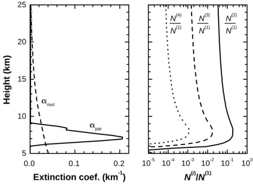
PSC observations is briefly addressed in the following, since it might be seen as a pos-sible source of error in the determination of PSC optical properties, particularly δ_par. We show that the multiple-scattering effect is negligible. We employed the multiple-scattering model described by Reichardt et al.(2000a) and Reichardt (2000) to sim-ulate the multiple-scattering contributions to the elastic lidar return signals from the

10

stratosphere. The cirrus extinction profile measured around 22:26 UT with the GKSS Raman lidar, and lidar parameters of this instrument were chosen for the simulations. Model results are shown in Fig.1. Second-order scattering is the dominant multiple-scattering effect, it contributes < ∼4% to the total lidar signal above 20 km. Since dou-bly scattered light experienced a single (direct) forward-scattering process in the cirrus

15

cloud that does not change the state of polarization, this signal augmentation does not affect the depolarization measurement in PSCs. Only backscattered light of higher scattering orders (two or more scattering processes in the cirrus clouds) might interfere with the δ_par determination, however, they are irrelevant in our case (scattering orders > 2 amount to less than 0.2% above 20 km). Finally, we want to point out that multiple

20

scattering in cirrus clouds does not play a role in measurements of PSC backscat-ter and lidar ratios either, because, respectively, the multiple-scatbackscat-tering contributions to elastic and Raman return signals cancel out (Wandinger,1998), and the ratios of multiply to singly scattered light depend only weakly on height in the stratosphere.

3. Meteorological setting

25

Results of a mesoscale model simulation illustrate the meteorological setting. The mesoscale fields are calculated with the non-hydrostatic weather prediction model

(10)

ACPD

MM5-version 3.4 (Dudhia, 1993; Dudhia et al., 2001). The outer model domain is centered at (65◦N, 20◦E) with an extension of 2457 km × 2457 km. In this domain a horizontal grid size of∆x = 27 km is used. A local grid refinement scheme (nested domains of 9 and 3 km horizontal resolution, respectively) is applied to resolve most of the horizontal wavenumber spectrum of vertically propagating gravity waves excited by

5

the orography.

The mesoscale simulation presented in this paper was performed with 128 vertical levels up to the model top at 10 hPa (∼30 km) which results in a high spatial resolution of∆z ≈ 230 m. More important for a correct modeling of the vertical propagation of mountain waves into the stratosphere, however, is the modified radiative top boundary

10

condition of Z ¨angl (2002) which is applied in the current MM5 version. This bound-ary condition reduces the reflection at the model top significantly (D ¨ornbrack et al.,

2002). Radiative and moist processes are switched off since the prime concern lies in the dynamics of mountain waves at upper levels. The initial conditions and boundary values of the model integration were prescribed by 6-hourly operational analyses of

15

the ECMWF model with a horizontal resolution of 0.5◦in latitude and longitude and 15 pressure levels between the surface and the 10-hPa pressure level.

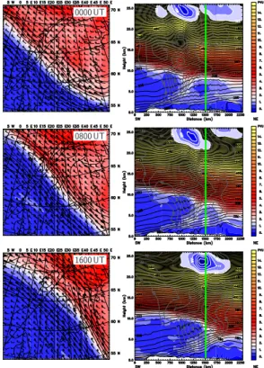
Figure 2 illustrates the simulated stratospheric temperature fields of the innermost model domain. Northern Scandinavia was located entirely inside the polar vortex on 16 January 1997. Inside the vortex the stratospheric temperature field at the isentropic

20

surface Θ = 550 K is rather uniform with T ≈192 K (over the Norwegian Sea in the horizontal sections of Fig.2). Vertically propagating mountain waves generate elon-gated stratospheric temperature anomalies parallel to the mountain ridge. As will be discussed later, hydrostatic gravity waves in the non-rotating regime with horizontal wavelengths ≤ 100 km lead to vertical displacements of isentropes directly above the

25

mountain ridge (compare the vertical sections in Fig. 2) whereas longer hydrostatic gravity waves in the rotating regime propagate also leeward (we use the terminology of Gill, 1982). At Θ = 550 K the local temperature deviates from the average tem-perature inside the polar vortex by up to 12 K. There are two dominating stratospheric

(11)

ACPD

temperature anomalies. At 00:00 UT, the horizontal distance between the westerly and the easterly one is about 150 km and increases to more than 400 km in the af-ternoon of 16 January 1997 (not within the display range of Fig. 2). Furthermore, the series of horizontal sections indicates an apparent downstream advection of the westerly cold anomaly towards the east. However, inspection of the vertical sections

5

reveals that the horizontal wavelength of the westerly temperature anomaly increases from less than 50 km at 00:00 UT to about 200 km at 16:00 UT. Consequently, also its position relative to the mountain range shifts leeward. This is due to the excita-tion of hydrostatic gravity waves in the rotating regime by the long-lasting flow past the Scandinavian mountain ridge (e.g.D ¨ornbrack et al.,1999,2002). These inertia-gravity

10

waves have a non-vanishing horizontal component of the group velocity, therefore they are able to produce stratospheric temperature anomalies in the lee of the mountain ridge. Their smaller vertical group velocity compared to non-rotating hydrostatic waves lead to about 5 to 10 times larger propagation times to stratospheric levels and to an increasing distance between the westerly and easterly temperature minima during the

15

day.

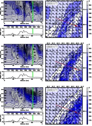
The coldest region inside the stratospheric temperature anomaly, however, propa-gates northward and is related to the position of the jetstream underneath. Figure3

depicts the tropospheric meteorological evolution above the Scandinavian mountain range on 16 January 1997. The prominent features are the northward-tilted tropopause

20

(the white band in the vertical sections corresponding to a potential vorticity (PV) value of 2 PVU) and the tropopause fold associated with a strong jetstream. The difference between the tropopause heights on the cyclonic and the anticyclonic side is about 6 km. The jetstream attains a maximum velocity of ∼60 ms−1in its core. In the course of time the tropopause fold and jetstream advance northward (see the horizontal sections of

25

PV and wind on the 308-K isentropic surface). Near-surface winds upstream of Scan-dinavia are nearly perpendicular to the main mountain ridge. They peak at maximum values of ∼20 ms−1 at 850 hPa between 00:00 UT and 12:00 UT and decrease after-wards significantly to values below 5 ms−1 (not shown). Hours later this weakening of

(12)

ACPD

the near-surfaces winds causes the wave activity in the stratosphere to decrease and eventually cease (after ∼18:00 UT, see Fig.4).

The key to understanding the lidar observations at Esrange and the associated stratospheric temperature structure lies in the position of the jetstream relative to the lidar site. The large vertical shear of the zonal wind U in the troposphere ∂U/∂z =

5

60 ms−1/8000 m= 7.5×10−3s−1 generates a Froude number profile F (z) = N h/U falling with altitude, where N is the buoyancy frequency (∼ 0.01 s−1) and h≈1500 m is the height of the Scandinavian mountain ridge. In such regions, vertical gravity wave propagation is significantly facilitated. As a consequence, the strongest stratospheric cooling due to mountain waves is locked with the position of the jetstream advancing

10

northward (see the stratospheric temperature anomaly in the vertical section of Fig.3). The minimum temperature drops from 186 K (00:00 UT) to less than 182 K (16:00 UT) in the mountain wave-induced stratospheric temperature anomaly. In summary, the enhanced wave activity above the jetstream leads to an extra cold region in an altitude range between 22 and 26 km which proceeds northward while the longer horizontal

15

mountain waves result in an eastward drift of the temperature anomaly.

4. PSC macrophysical properties

The stratospheric temperature field downstream the Scandinavian mountains can be best described as a series of temperature minima parallel to the ridge whereby the in-tensity of mountain wave cooling is modulated by synoptic-scale (jetstream dynamics)

20

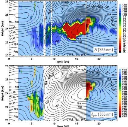
and mesoscale (wave propagation) processes (Fig.2). As the result of the combined synoptic and mesoscale dynamics, the height versus time representation of the temper-ature above Esrange resembles a distorted quadrupole field, with the 192-K isothermal lines being the center axes (Fig.4). In the morning of 16 January 1997, stratospheric conditions at the lidar site are governed by the easterly mountain wave-induced

tem-25

perature anomaly leading to temperatures warmer and colder than 192 K at heights below and above ∼ 23 km, respectively. Due to the long-lasting flow past the mountain

(13)

ACPD

ridge and the associated dilatation of the horizontal wavelength this pattern reverses over time. At ∼ 07 : 00 UT, the stratosphere between 21 and 27 km is nearly isothermal at T = 192 K. Later on, the intensifying westerly temperature anomaly dominates the temperature field over Esrange with temperatures colder below, and warmer above, the sloping 192-K isotherm.

5

The observed PSC evolution above Esrange is mostly related to the development of the westerly stratospheric temperature anomaly, only the isolated PSC patches de-tected at altitudes > 25 km in the early morning between 02:00 UT and 06:00 UT are probably generated at the windward edge of the easterly temperature minimum. The main PSC event, however, starts around 04:00 UT when first particle backscattering is

10

measured at 23.5–24 km. Over the next 2 h the PSC cloud base lowers to minimum heights around 20.5 km. This correlates with a decrease in temperature at altitudes < 23 km. Afterwards, PSC base and top move steadily upwards by ∼170 m/h un-til 19:30 UT with the geometrical thickness of the PSC remaining nearly constant at ∼3 km. The simulated mountain wave-induced stratospheric anomaly also shows this

15

upward propagation.

PSC optical data before 07:40 UT reveal a growth of R and a reduction of δ_par with decreasing temperature. The change is particularly pronounced at sunrise around 06:40 UT. This transition in PSC optical signature, which is discussed in greater detail in Sect.5.1, suggests that scattering by liquid ternary aerosol (LTA) droplets increasingly

20

dominates scattering by solid particles, most likely consisting of nitric acid trihydrate (NAT; the leading edge of the PSC follows quite well the NAT equilibrium temperature T_NAT).

After sunrise and until ∼17:00 UT, R values continue to increase while the ambient air masses are cooling. Backscatter spikes at 24 km between 09:00 UT and 11:30 UT

25

are probably caused by PSC patches consisting predominantly of ice particles II PSC) rather than by LTA droplets Ib PSC) or crystalline NAT particles (type-Ia PSC) because R values clearly exceed those expected for type-I PSCs. If this interpretation was correct, we would have observed ice particles that were nucleated

(14)

ACPD

previously in the core of the westerly temperature minimum ∼80 km upstream and that survived advection to the lidar site in subsaturated air (temperatures are several degrees Kelvin above the ice equilibrium temperature T_ice), albeit evaporating. The hypothesis of subliming ice particles being the cause for the backscatter maxima before 11:30 UT is supported by the observation of a PSC region with even larger R values

5

entering the lidar field of view around noon at similar heights in air masses still warmer than T_ice, that increases in vertical extent to both lower and higher altitudes over time while the stratosphere below 26 km is cooling until T_ice is reached around 13:00 UT.

Between 13:00 UT and ∼18:00 UT the cold core of the westerly temperature anomaly resides directly above Esrange. The mesoscale simulation indicates minimum

temper-10

atures of 181 K at 24 km which is about 3 K below the frost point. Therefore one can conclude that the extreme backscatter ratios (> 25 at 355 nm, > 150 at 532 nm) and particle depolarization ratios (> 0.5) measured by the two lidars are the optical signa-ture of a PSC II in the early stages of its life cycle with possibly newly nucleated, and growing ice particles.

15

After 18:00 UT wave activity weakens leading to an upstream shift of the attenu-ating temperature minimum. The Esrange lidars monitor the outflow of the westerly temperature anomaly again. Around 19:00 UT the PSC collapses to a 0.5-km wide layer. Associated with the change in geometrical properties is a drastic transition in PSC backscatter and particle depolarization ratios. The slowly subsiding thin PSC

20

clearly exhibits the optical characteristics of a PSC Ib (LTA droplets), except for short-lived patches around 20:00 UT with elevated δ_par. Apparently, the windward temper-ature minimum shallowed to such an extent that nucleation of solid particles is sig-nificantly reduced. Wave-processing foremost results in growth and evaporation of the liquid aerosol. These droplets may have originated from the synoptic PSC I that

25

was observed at the same time at similar heights on the weather side of the Scandi-navian mountain ridge over the research facility ALOMAR approximately upwind Es-range (Fricke et al.,1999). The transition from PSC II to PSC Ib as observed between 17:00 UT and 20:00 UT over Esrange will be discussed in more detail in Sect.5.2.

(15)

ACPD

In summary, the following interpretation of our ground-based lidar measurements in terms of temporal evolution of the PSC can be given. The dominant mountain wave-induced temperature anomaly develops first upwind and then above Esrange. In the morning and until the early afternoon while wave activity intensifies and horizontal wavelength increases, the quasi-stationary PSC extends into the field of view (trailing

5

edge first), thus leading to a time-reversed observation of PSC evolution: later stages of particle history are observed before earlier stages. First, NAT particles are detected as the outflow from the westerly wave-induced PSC at relatively warm temperatures (all LTA droplets or ice particles are evaporated). Then, as the cold core of the wave expands eastward (due to wave dynamics) and northward (due to jetstream dynamics),

10

more and more LTA droplets and, after 09:00 UT, ice particles appear above the lidar site, causing the PSC optical signature to change from PSC Ia over PSC Ib to PSC II. The earliest stage of PSC particle history is observed around 17:00 UT when ice par-ticles are nucleated directly above Esrange. Later on, as the wavelength shortens and the temperature anomaly moves westward again, lidar measurements are in sync with

15

the temporal PSC particle evolution: earlier stages are observed before later stages. The microphysical analysis in Sect.5.3shows that the retrieved ice particle sizes de-crease with time, probably due to a diminishing growth rate and eventually evaporation. With the cessation of particle nucleation upwind, the major mountain wave PSC event over Esrange comes to an abrupt end. All that remains is a wave-processed synoptic

20

PSC Ib that is observed until lidar operation is ended at 03:10 UT on 17 January 1997. Interestingly, the wave PSC as monitored above Esrange does neither exhibit a lam-inated vertical structure nor a temporal or spatial oscillatory pattern which are common features of this PSC type otherwise when observed with airborne lidars (e.g.Wirth et

al., 1999; D ¨ornbrack et al., 2002). Given the meteorological setting on 16 January

25

1997, it is probable though that similar features would have been detected if there had been a lidar-equipped aircraft observing the PSC along a flight track parallel to the main tropospheric wind direction (e.g. with a ground track similar to the base of the vertical section of Fig.2).

(16)

ACPD

5. PSC microphysical properties

In this section we present the results of our microphysical studies that helped us derive the general interpretation of our lidar measurements on 16 January 1997 given before. It has to be pointed out, however, that a full assessment of PSC microphysics cannot be expected from our analysis. The relation between PSC microphysical and optical

5

properties is complicated. In previous studies of PSC measurements acquired with air-borne lidars, coupled optical and microphysical modeling was employed to counter this problem (e.g.Carslaw et al.,1998b;Wirth et al.,1999). The success of this approach is in part due to the relatively simple observation geometry of the measurements, as explained before. In order to apply this technique to PSC measurements with

ground-10

based lidar instruments, however, one would have to take into account the time-space convolution of the observation which would require coupling of optical, microphysical and, additionally, dynamical models. Currently, such an extensive model is not avail-able to us.

In our discussion we focus on the two major events that were captured with the GKSS

15

Raman lidar, specifically, these are the transitions in the PSC optical characteristics from PSC Ia (with enhanced R) to PSC Ib (04:00–09:00 UT), and from PSC II to PSC Ib (17:00–20:00 UT).

5.1. PSC observations in the morning of 16 January 1997

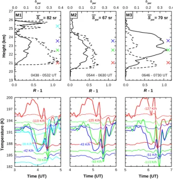
Figure 5 displays the evolution of the PSC backscatter-ratio and depolarization-ratio

20

profiles in the morning of 16 January 1997. To increase the precision of the S_par deter-mination, lidar data are summed over three consecutive measurement intervals M1– M3 with relatively little variation in PSC optical and geometrical properties. Generally, δ_par and S_par decrease, and R increases, with time although some exceptions exists. For example, cloud-base δ_par values measured during interval M3 are similar to those

25

observed during interval M2. Apparently, LTA droplets that depress δ_par at the PSC altitudes above are smaller in number, small in size, or completely absent here.

(17)

In-ACPD

terestingly, S_par values of intervals M2 and M3 are comparable despite the significant change in the fractional contributions of crystalline and liquid particles to PSC light scattering (see Fig.6). It is possible that opposing trends in the temporal development of solid-particle and droplet S_par simply cancel out, however, as we will discuss later, decomposition of the PSC optical signature into particle-type specific optical

proper-5

ties as well as microphysical considerations suggest instead that the solid and liquid particles present have similar lidar ratios that change little over time.

To facilitate interpretation of the lidar measurements, backward trajectories based on mesoscale simulation fields were calculated. Air parcel temperature histories are presented in Fig.5for selected PSC heights. Only the last 2 h prior to the lidar

obser-10

vations are shown. The mountain wave induced several cycles of cooling and heating of which, in the case of the main PSC layer between 20 and 25 km, the most pro-nounced occurred 30 min before the observations. In this temperature anomaly of rather short duration, the air masses are cooled by several degrees Kelvin to minimum temperatures with high cooling rates (particularly during measurements M2 and M3

15

at heights < 23 km), but fail to reach in all but one case (22.5 km, measurement M3) temperatures 3–4 K below the frost point (assuming 5 ppmv H₂O) which is generally regarded as the threshold temperature range for solid-particle nucleation (Tabazadeh

et al.,1997;Carslaw et al.,1998b).

Since the question whether or not temperatures dropped sufficiently to allow ice

par-20

ticles to form is important for understanding the PSC event over Esrange, it has to be carefully addressed. Several explanations are conceivable. First, the simulated mesoscale minimum temperatures are accurate and the assumed water vapor con-tent is about right. This would mean that indeed no solid particles nucleated in the mountain wave. Particle depolarization ratios measured during measurements M1–

25

M3 would be due to solid particles already present upwind the Scandinavian mountain ridge that served as condensation nuclei while being transported through the tem-perature anomaly. According to synoptic-scale trajectory calculations based on the operational ECMWF analyses (not shown), the air parcels detected at 30 hPa crossed

(18)

ACPD

the southern tip of Greenland 24 h before the measurements, and maintained temper-atures < T_NAT afterwards. Hence it is possible that the advected air was processed in a mountain wave over Greenland at that earlier time (Carslaw et al.,1998a), and that solid condensation nuclei preexisted. Second, the temperature simulations are correct, but stratospheric humidity is underestimated. If the water vapor concentration was, e.g.

5

about 7 ppmv rather than 5 ppmv, T_ice would rise by ∼ 1.5 K increasing the likelihood of ice particle nucleation significantly. Third, simulated mesoscale temperatures are too warm. In the morning of 16 January 1997, this effect would be aggravated if the small-scale structure of the temperature anomaly were not fully resolved by the model. The studies ofLarsen et al.(2002) andFueglistaler et al.(2003) show that the

discrep-10

ancies between simulated and measured temperatures can be several degrees Kelvin, with the mesoscale model temperatures consistently being warmer. In our case, a tem-perature correction of −1 to −3 K (depending on height) would be required to trigger ice nucleation both in the morning (Fig.5) and the afternoon (Fig.7) of 16 January (all other parameters unchanged), which is in the range of temperature correctionsLarsen 15

et al. (2002) had to apply to match microphysical simulations and observations. The assessment that model temperatures may be too warm is corroborated by the obser-vation of large amounts of LTA above 22 km in measurement interval M3. Our model simulations yield temperatures within 1 K below T_NAT in the LTA layer, while the theo-retical work ofCarslaw et al. (1994) on equilibrium growth of liquid aerosol show that

20

LTA volume does not increase significantly unless temperatures fall several degrees Kelvin below T_NAT. In summary, in view of the accuracy of the mesoscale numerical simulations and the uncertainties associated with the stratospheric trace gas concen-trations, we consider it very likely that mountain wave temperatures actually fell below the nucleation threshold of ice particles, and that solid particles subsequently formed.

25

Preexisting solid particles may have aided PSC formation as additional condensation nuclei.

As discussed previously, the transition in PSC optical properties observed in mea-surements M1–M3 is the result of changes in the size distributions of the coexisting

(19)

ACPD

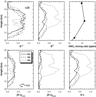
solid and liquid particles. The main cause is the decrease in temperature in general, and above Esrange in particular, with time, allowing the LTA droplets to grow to larger volume in the mountain wave, and to maintain larger sizes during their subsequent ad-vection to the lidar site (Fig.5). The different trends in the evolution of the two particle types are visible in the ratios of polarized particle backscatter coefficients to

molec-5

ular backscatter coefficient (Fig. 6). Bk indicates the significant temperature-related increase in droplet volume while, in contrast, B⊥ exhibits little variability. From the spa-tial and temporal homogeneity of B⊥ the important conclusion can be drawn that the optical and microphysical properties of the crystalline particles are similar throughout the vertical extent of the PSC and remain unchanged during measurement intervals

10

M1–M3. Consequently, the most accurate measurement of the depolarization ratio of scattering by these solid particles, δ_parsolid, is obtained at heights and times where tem-peratures are too warm for liquid particles to exist in significant amounts. This condition should be approximately met in measurement M1, and we obtain δ_parsolid = 0.3 ± 0.05. With this estimate we are able to calculate the contributions of solid and liquid

parti-15

cles to the PSC backscatter ratio. Using the defining equations of B⊥, Bk, and δ_parsolid (δ_parliquid= 0), we obtain

(R − 1)_solid= B⊥(1+ 1/δ_parsolid), (4)

(R − 1)_liquid= Bk− B⊥/δ_parsolid, (5)

with R −1= (R−1)solid+(R−1)liquid. The results of the computations are shown in Fig.6.

20

Solid-particle scattering dominates measurements M1 and M2; the low (R − 1)_liquid values may either indicate scattering by few or small coexisting LTA droplets, or be the residual of our computations if δ_parsolid was overestimated. In contrast, (R − 1)_liquid (R − 1)_solidis found in measurement M3 for heights > 22 km. Interestingly, heights of highest (R − 1)_liquidvalues and maximum HNO₃concentrations coincide (Fig.6).

25

We mentioned before that S_par values of measurements M2 and M3 are similar. Since our trend analysis suggests that the optical properties of the solid particles

(20)

re-ACPD

main the same, this must also be the case for the LTA droplets, despite the fact that a significant size change occurred from one measurement to the other. Surprising as it first may sound, this finding can be explained if an increase in the refractive index of the droplets upon evaporation is taken into account (Sect.5.3). For this reason, we will assume S_par = (70 ± 14) sr (20% systematic error, see Sect.2) for both crystalline

5

PSC particles (δ_parsolid = 0.25–0.35, measurements M1–M3) and liquid PSC particles (δ_parliquid = 0, measurement M3) in our retrieval of microphysical properties. The el-evated S_par value measured during time period M1 is not considered representative of the solid particles, since the appearance of an isolated and short-lived PSC patch around 25.5 km (Figs.4and5) might affect the accuracy of the Spar measurement for

10

the main PSC layer.

While it is straightforward to assume that the liquid particles consist of aqueous so-lution of HNO₃ and H₂SO₄ (LTA), the composition of the solid PSC particles is not that obvious. If ice particles grew to large sizes in the cold core of the mountain wave, it appears possible that these particles survived transport in subsaturated air

15

until they were detected above Esrange after 30 min, although the heating rates were very high. However, if this hypothesis were true one would expect to see a correla-tion between B⊥ and the temporal evolution of the temperature profile, which is not observed. Therefore we assume that the solid particles consisted of NAT, although hydrates with higher H₂O:HNO₃ molar ratio might have been present also (Marti and 20

Mauersberger,1993). We would like to point out, however, that in situ data generally confirm the existence of NAT particles in the stratosphere (Fahey et al.,1989;Kawa et

al.,1992;Voigt et al.,2000), in one measurement case that is similar to ours about 2 h downwind mountain wave-induced solid-particle nucleation (Voigt et al.,2000;Larsen

et al.,2002;D ¨ornbrack et al.,2002;Schreiner et al.,2002).

(21)

ACPD

5.2. PSC observations in the afternoon of 16 January 1997

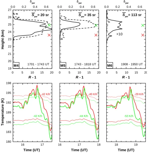
Figure7shows our PSC measurements during and shortly after the core of the moun-tain wave-induced temperature anomaly resided over Esrange. PSC optical signatures are remarkably different from those observed earlier (Fig. 5). During measurements M4 and M5, R and δ_par reach maximum values of, respectively, 10–20 and 0.5–0.65,

5

while S_par decreases to 20–35 sr. These optical characteristics, which are similar to those of cirrus clouds (Reichardt et al.,2002a), leave no doubt that the PSC consisted of large water-ice particles (PSC type II). Concurrent lidar measurements upwind Es-range on the weather side of the Scandinavian mountains reveal the existence of only a weak PSC (at 24 km, R < 2 at 532 nm;Fricke et al.,1999), which implies that the

10

ice particles formed on their way between both sites. The temperature histories con-firm cooling of the advected air masses of up to 15 K. Considering our discussion of temperature errors in Sect.5.1, it thus seems probable that the temperatures got cold enough for ice-particle nucleation, and that the lidars at Esrange were actually monitor-ing this process durmonitor-ing time periods M4 and M5 in the main PSC layer. Below 24.2 km

15

during measurement M5, however, the meteorological conditions must have been dif-ferent since R and δ_parare significantly smaller. The δ_parvalues of 0.05–0.1 may result from scattering by predominant LTA droplets that are in coexistence with either pre-existing solid particles, or a small number of ice particles nucleated but in the largest supercooled droplets.

20

Considering measurement M6, we favor the latter interpretation. Here maximum supercooling with respect to ice and the PSC optical properties of the main layer around 25 km are comparable to those of observation M5 at ∼ 23.5 km. At these lower heights, however, no δ_par > 0 is detected during measurement M6, indicating that a slight warming of ∼ 1 K (compared to the temperature data of observation M5 at 23.5 km)

25

is sufficient to suppress depolarization. This would not have been the case if solid particles had existed upwind the mountain wave.

(22)

domi-ACPD

nates, analysis of B⊥ and Bk does not yield any additional information and is, there-fore, not shown. Finally, we would like to point out that the modeled cooling rates of measurements M4–M6 are significantly lower (in absolute values) than those of mea-surements M1–M3. For that reason, it can be expected that the number density of nucleated ice and NAT particles is lower in the afternoon than in the morning because

5

a smaller fraction of the population of supercooled droplets can freeze (Larsen et al.,

2002;Fueglistaler et al.,2003). 5.3. Microphysical retrieval

In the following, PSC microphysical properties retrieved from the lidar measurements are discussed. The analysis first focuses on solid particles, specifically those observed

10

during measurement intervals M1–M3, M4 and M5.

Estimates of particle shapes, sizes, and number concentrations are obtained by com-paring measurements and theoretical optical data. For the first time S_par is used in the retrieval next to δ_par. Lidar ratio and particle depolarization ratio are two optical prop-erties that ideally complement one another because they contain different information

15

about the scattering matrix of the PSC particle ensemble. Both are independent of the particle number concentration and thus can be directly used to infer particle micro-physical characteristics. Different principal particle shapes are investigated. Studies byLiu and Mishchenko(2001) andReichardt et al.(2002c) demonstrate that retrieval results depend strongly on the assumed shapes of the particles, but to our knowledge

20

PSC observations with lidar were analyzed by use of a spheroidal particle model only (Carslaw et al., 1998b; Tsias et al., 1999; Wirth et al., 1999;Flentje et al., 2002;Hu

et al.,2002;Fueglistaler et al.,2003). In this study we compare the lidar data to the optical properties of spheroids, hexagons, and, for the first time, particles without any symmetry (irregular particles). It is assumed that the size distribution of the optically

25

relevant PSC particles is narrow. In the case of mountain wave PSCs this approxima-tion is justified as in situ measurements (Voigt et al., 2000), microphysical modeling

(23)

ACPD

(Tsias et al., 1999; Larsen et al., 2002), and size-spectrum-resolved retrievals from lidar data (Tsias et al., 1999; Wirth et al., 1999; Toon et al., 2000; Hu et al., 2002) confirm. Lidar measurements at multiple wavelengths are not available (see Sect.2), therefore color ratio cannot be included in our analysis.

Solid particles are assumed to consist of NAT, or ice. For NAT a refractive index of

5

1.53 as observed byDeshler et al.(2000) is chosen, for ice the data ofWarren(1984) are used (refractive index of 1.32 at 355 nm). Phase matrices of hexagons and irreg-ular particles are calculated with the finite-difference time-domain method described by Yang et al. (2000). Scattering properties of spheroids with aspect ratios (defined as the ratio of length to diameter of the particle) smaller or larger than one are

calcu-10

lated according to the T-matrix technique (Waterman,1970). The computer code used is available athttp://www.giss.nasa.gov/∼crmim/t matrix.html(Mishchenko,1991). Mie theory is applied to determine the phase functions of spheres (van de Hulst,1981). For a discussion of the optical constants selected, and for more details about the compu-tations seeReichardt et al.(2002c).

15

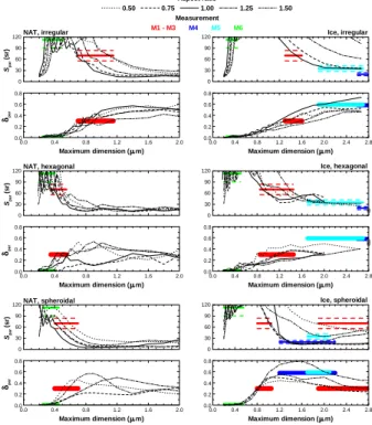
Figure 8 compares measured and theoretical optical properties of solid PSC parti-cles. Theoretical lidar ratio and particle depolarization ratio are plotted versus the max-imum dimension of the particles. Measurements are visualized with solid horizontal lines. In the case of δ_par, the line thickness reflects the variability of the observed PSC profile. Dashed horizontal lines show estimated systematic errors of S_par. Lengths and

20

positions of the horizontal lines indicate particle size ranges with best-possible agree-ment between observations and theoretical data. The size ranges are relatively well defined in most cases, despite the fact that only two optical properties are available to constrain the retrieval. The reason for the stability of the solutions is the opposite dependence of δ_par and S_par on particle maximum dimension. Only if the particles are

25

much larger than the observation wavelength, as it is the case in measurements M4 and possibly in M5, S_parand δ_parare not sensitive to changes in particle size any more, and the retrieval results become unstable.

(24)

agree-ACPD

ment between measured and theoretical optical data is found for irregular NAT and hexagonal ice particles. Nevertheless we can exclude the ice particles from our analy-sis if we take into account that in the morning of 16 January ambient temperatures were significantly warmer than T_ice, and that a well developed hexagonal symmetry is rather unlikely for small ice particles with 0.8–1.4 µm maximum dimension anyway. Examining

5

the optical data of irregular NAT particles closer, we find that the particles most likely had maximum dimensions between 0.7 and 0.9 µm and aspect ratios between 0.75 and 1.25 or sizes of about 1.1 µm with either small (0.5) or large (1.5) aspect ratios. However, these latter particles can be discarded because their aspect ratios should be too extreme for micron-size particles.

10

From (R − 1)_solid≈ 0.3 it then follows that the particle number density was n_NAT = 8– 12 cm−3, and that condensation of gas-phase HNO₃ was equivalent to 4.5–7.6 ppbv which was 31–55% of the total amount of available HNO₃ (generally, retrieval results are such that small maximum dimensions correspond to high number densities and small amounts of condensed HNO₃, and vice versa). A summary of all measured

15

optical and retrieved microphysical properties is given in Table1.

The retrieval results are consistent with those of previous studies of solid-particle PSCs downwind mountain waves. Toon et al. (2000) infer from dual-wavelength po-larization lidar data of Arctic PSCs high number densities (comparable to those of the condensation nuclei n_CN) of NAT particles < 1 µm, leading to a depletion of the

20

gas-phase HNO₃ reservoir. Coupled microphysical and spheroid model-based optical modeling was performed byCarslaw et al.(1998b),Tsias et al.(1999), andWirth et al.

(1999). Comparison with the results of the latter investigation is particularly instructive, because the PSC event studied is similar to our 16 January 1997 observation regard-ing the location of the NAT PSC in close proximity to the upwind ice PSC, and the

25

high cooling rates. Wirth et al. (1999) report particle sizes of 0.6–0.7 µm which is in agreement with our analysis for NAT spheroids (see Fig.8), but which is smaller than our final retrieval results obtained for irregular NAT particles. This finding nicely illus-trates the dependence of any microphysical retrieval on particle shape assumptions.

(25)

ACPD

Cooling rates and number densities of nucleated NAT particles seem to be correlated. In our case, maximum cooling rate at PSC center is 113 K/h (measurement M3) and n_NAT = 8–12 cm−3,Wirth et al.(1999) report cooling rates of up to 60 K/h and n_NAT = 3– 6 cm−3, whileCarslaw et al.(1998b) find much less particles per volume in the outflow of the mountain wave PSC with cooling significantly less rapid (Wirth et al., 1999).

5

Recent in situ measurements (Voigt et al.,2003) as well as mesoscale/microphysical modeling (Fueglistaler et al.,2003) of mountain wave PSCs yield a similar dependence of n_NAT on cooling rate. Finally, Tsias et al.(1999) obtain NAT particle sizes < 1 µm which is consistent with our analysis.

M4 and M5 observations are compared to theoretical optical data of ice crystals

10

only, since the elevated backscatter ratios are too high for PSCs consisting of NAT particles, even for those generated by mountain waves (Tsias et al.,1999;Reichardt et

al.,2000b). M4 depolarization ratios agree well with δ_parvalues of irregular ice particles > 1.9 µm, but measured lidar ratios are smaller than the theoretical data, even for a particle maximum dimension of 2.7 µm. If a hexagonal particle shape is assumed, M4

15

measurements do not fit the FDTD results for particle sizes < 2.7 µm, but are close to the theoretical values obtained in the geometrical-optics approximation for columnar hexagons with aspect ratios between 1 and 2.5. This similarity implies that the particles observed during measurement interval M4 were large, probably 3 µm. Since only a lower limit of the particle size can be given, particle number concentration can only be

20

estimated. If n_icewere 5 and 10 cm−3as retrieved byHu et al.(2002) andFueglistaler

et al. (2003), the corresponding particle sizes would be, respectively, 4.3 and 3 µm for irregular, and 2.8 and 2 µm for hexagonal ice particles. Of these, only the 4.3-µm irregular particles appear to be consistent with the optical data which leads us to the conclusion that n_icemust have been ≤ 5 cm−3.

25

In the case of measurement M5, observation and theory are in excellent agreement for isometric and slightly oblate irregular ice particles (aspect ratios of 0.75 and 1) with sizes > 1.9 µm. Theoretical S_parvalues of hexagons indicate similar particle maximum dimensions, yet measured and calculated δ_pardisagree. Again, the upper boundary of

(26)

ACPD

the particle size range cannot be retrieved because our observation at 355 nm are lack-ing sensitivity to size for large particles. For a more accurate size estimate, observa-tions at longer wavelengths would be needed. The lower limit of the particle maximum dimension (> 1.9 µm) confines the particle number density to n_ice < 27 cm−3. This upper boundary is probably too high for two reasons. First, n_ice should not be larger

5

than the number concentration of the background aerosol, but maximum n_CN values measured in (mountain wave) PSCs are, to our knowledge, about 20 cm−3 (Larsen et

al.,2002). Second, our retrieval yields smaller particle number densities for all other measurement intervals. Contrarily, assuming a concentration of the ice particles similar to the estimated number densities of the NAT (M1–M3) and the LTA (M3, M6) particles

10

(n_ice = 8–11 cm−3, Table 1) and assuming an irregular isometric shape, we retrieve particle sizes in the range of 3 to 3.5 µm which are likely to be consistent with the PSC optical properties of measurement M5.

Assuming spheroidal particle shapes, we retrieve a mixture of slightly oblate and prolate particles (aspect ratios of 0.75 and 1.25) for the PSC observed during

mea-15

surement M4. In the case of observation M5 the agreement between theoretical and observed data is rather poor. In contrast to the results obtained for irregularly shaped crystals and hexagons, the spheroidal particle model yields both lower and upper bounds of particle size and concentration for measurements M4 and M5. However, the retrieved particle sizes (< 2.2 µm) appear somewhat small for ice PSCs.

20

Finally, we analyze measurement M6 because, in theory, the optical signature of this PSC (δ_par < 5%, S_par = 113 sr) could stem from scattering by solid particles alone. In-dependently of particle composition and shape, observed and calculated optical prop-erties agree well for particle maximum dimensions between 0.2 and 0.5 µm. However, to explain the backscatter ratio of 1.7 with these small particles, one would have to

as-25

sume number concentrations that are not realistic (n_ice > 150 cm−3, n_NAT > 65 cm−3). Thus we conclude that during measurement interval M6 solid and liquid PSC particles coexisted, and that LTA droplets dominated light scattering.

(27)

ACPD

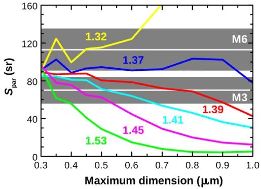
355-nm theoretical data. Different chemical compositions of the LTA droplets were assumed in the Mie computations. In the stratosphere, an increase in temperature is related to a decrease in the water contents of the ternary solution and, thus, to an increase in LTA refractive index. In the UV it varies between 1.37 (85 wt% H₂O, T ≈ T_ice− 4 K) and 1.45 (55 wt% H₂O, T ≈ T_ice+ 3 K) (Carslaw et al.,1994;Luo et al.,

5

1996).

It is important to note that refractive indices between 1.39 and 1.53 correspond to diameters between 0.85 and 0.35 µm, respectively, for an assumed lidar ratio of 70 sr. Therefore it seems possible that the lidar ratio of a population of LTA droplets evapo-rating due to warming temperatures remains relatively unchanged, as we assumed to

10

explain the almost identical S_par values of measurement intervals M2 and M3.

The optical data also show that the refractive index of the LTA droplets was smaller in measurement M6 than during the earlier observation M3, which is in accordance with the mesoscale numerical simulation of colder PSC temperatures for the afternoon. The relatively high backscatter ratios of 1.6–1.7 in both cases require the droplets sizes to

15

be large since otherwise droplet concentrations would be too high. Considering tem-perature and R values, we infer an LTA refractive index of 1.39, droplet diameters of 0.7–0.9 µm, and particle concentrations of 7–11 cm−3for measurement M3. These val-ues correspond with condensation of 3.7–4.8 ppbv HNO₃out of the gas phase. Com-bining the results of our microphysical retrieval for LTA and NAT particles, we obtain a

20

total particle number density of 15–23 cm−3. Given the high stratospheric cooling rates in the morning of 16 January 1997, it appears likely that about all of the supercooled droplets nucleated ice particles in the mountain wave upwind Esrange, which would mean that on ∼ 53% of these particles ice-mediated nucleation of NAT occurred (the remaining ∼ 47% of the ice particles released liquid droplets after ice evaporation).

25

Wirth et al.(1999) report a similar fraction for a mountain wave PSC with comparable cooling rates. The total amount of condensed HNO₃ sums up to 8.2 to 12.4 ppbv, i.e. 57–90% of the HNO₃gas reservoir. This compares well with the microphysical model results obtained for the mountain wave PSC studied byVoigt et al. (2000); Larsen et

(28)

ACPD

al. (2002);D ¨ornbrack et al.(2002);Schreiner et al. (2002). According toLarsen et al.

(2002), depletion of the HNO₃ gas reservoir can reach 100% in the ice PSC, and de-creases downwind. About 1 h after the air parcels warmed up to temperatures > T_ice, depletion between 40% and 90% is found, depending on altitude (Larsen et al.,2002). For measurement M6, best agreement between PSC observation and theoretical

5

data is found for water-rich LTA droplets (refractive index of 1.37) with diameters be-tween 0.7 and 0.9 µm and a number density of 9–10 cm−3. The amount of condensed HNO₃ (3.4–6.5 ppbv) is similar to the value retrieved for the LTA droplets of measure-ment M3. However, total reduction of gas-phase HNO₃is less pronounced than in the latter case, since solid NAT particles do not contribute significantly. The reason for this

10

is unclear, but one could speculate that the time span between particle nucleation and lidar observation was too short to permit the NAT particles to grow to optically relevant sizes (compare Figs. 5and 7). In addition, cooling rates were lower in the afternoon than in the morning, so probably fewer NAT particles nucleated (Wirth et al., 1999;

Fueglistaler et al.,2003). Finally, we note that retrieved LTA number densities of

mea-15

surements M3 and M6 agree well with those reported previously (Voigt et al.,2000;

Biele et al.,2001;Hu et al.,2002), while droplet diameters appear to be slightly larger (Voigt et al.,2000;Hu et al.,2002).

6. Summary

The clarification of the mechanisms that lead to the formation and dissipation of

moun-20

tain wave-induced PSCs and the assessment of their microphysical properties will help to better understand stratospheric ozone chemistry. Our study demonstrates that ground-based lidar measurements can contribute to this endeavor if mesoscale mete-orological modeling is employed to resolve the space-time ambiguity of the observa-tions. In our approach, PSC microphysical properties are retrieved by comparison of

25

the measured particle depolarization ratio and PSC-averaged lidar ratio to theoretical optical data obtained for different particle shapes. It is found that for relatively small