The Herschel first look at protostars in the Aquila Rift

November 8, 2018

Letter to the Editor

The Herschel

?

first look at protostars in the Aquila Rift

??

S. Bontemps

, Ph. Andr´e

, V. K¨onyves

, A. Men’shchikov

, N. Schneider

, A. Maury

, N. Peretto

, D.

Arzoumanian

, M. Attard

, F. Motte

, V. Minier

, P. Didelon

, P. Saraceno

, A. Abergel

, J.-P. Baluteau

, J.-Ph.

Bernard

, L. Cambr´esy

, P. Cox

, J. Di Francesco

, A. M. Di Giorgo

, M. Gri

ffin

, P. Hargrave

, M. Huang

, J.

Kirk

, J. Li

, P. Martin

, B. Mer´ın

, S. Molinari

, G. Olofsson

, S. Pezzuto

, T. Prusti

, H. Roussel

, D. Russeil

,

M. Sauvage

, B. Sibthorpe

, L. Spinoglio

, L. Testi

, R. Vavrek

, D. Ward-Thompson

, G. White

, C.

Wilson

, A. Woodcraft

, and A. Zavagno

(Affiliations can be found after the references) Received ; accepted

ABSTRACT

As part of the science demonstration phase of the Herschel mission of the Gould Belt Key Program, the Aquila Rift molecular complex has been observed. The complete ∼ 3.3◦

× 3.3◦

imaging with SPIRE 250/350/500 µm and PACS 70/160 µm allows a deep investigation of embedded protostellar phases, probing of the dust emission from warm inner regions at 70 and 160 µm to the bulk of the cold envelopes between 250 and 500 µm. We used a systematic detection technique operating simultaneously on all Herschel bands to build a sample of protostars. Spectral energy distributions are derived to measure luminosities and envelope masses, and to place the protostars in an Menv− Lbolevolutionary diagram. The

spatial distribution of protostars indicates three star-forming sites in Aquila, with W40/Sh2-64 HIIregion by far the richest. Most of the detected protostars are newly discovered. For a reduced area around the Serpens South cluster, we could compare the Herschel census of protostars with Spitzerresults. The Herschel protostars are younger than in Spitzer with 7 Class 0 YSOs newly revealed by Herschel. For the entire Aquila field, we find a total of ∼ 45 − 60 Class 0 YSOs discovered by Herschel. This confirms the global statistics of several hundred Class 0 YSOs that should be found in the whole Gould Belt survey.

Key words.Stars: formation – Stars: luminosity function, mass function – ISM: clouds

1. Introduction

During the main accretion phase, protostars are deeply embed-ded in their collapsing envelopes and parent clouds. They are so embedded that they radiate mostly at long wavelengths, making their detection and study difficult from the ground (e.g. Andr´e et al. 2000; Di Francesco et al. 2007). Protostars, or young stellar objects (YSOs), in the solar neighborhood have been extensively surveyed, but a complete and unbiased census of all protostars in nearby molecular clouds is lacking. The census of embedded YSOs provided by IRAS and near-IR studies in the 1980s and 1990s was far from complete even in the nearest clouds. Thanks to their high sensitivity and good spatial resolution in the mid-infrared, ISO and, more recently, Spitzer could perform more complete surveys in all major nearby star-forming regions (e.g. Nordh et al. 1996; Bontemps et al. 2001; Kaas et al. 2004; Allen et al. 2007; Evans et al. 2009). The population of the youngest protostars, the Class 0 YSOs, can however not be properly sur-veyed solely in the near and mid-infrared. These youngest ob-jects remain weak or undetected shortward of ∼ 20 µm.

The Herschel Gould Belt Survey (Andr´e et al. 2010) is a key program of the ESA Herschel Space Observatory (Pilbratt et al. 2010). It employs the SPIRE (Griffin et al. 2010) and PACS (Poglitsch et al. 2010) instruments to do photometry in

large-? _{Herschelis an ESA space observatory with science instruments}

provided by European-led Principal Investigator consortia and with im-portant participation from NASA.

??

Figures 2–3 are only available in electronic form at http://www.aanda.org.

scale far-infrared images at an unprecedented spatial resolution and sensitivity. The Aquila Rift region has been chosen to be observed for the science demonstration phase of Herschel for this survey.

Our 250/350/500 µm SPIRE and 70/160 µm PACS images of the Gould Belt provide the first access to the critical spec-tral range of the far-infrared to submillimeter regimes to cover the peak of the spectral energy distributions (SEDs) of the cold phase of star formation at a high enough spatial resolution to sep-arate individual objects. The Herschel surveys therefore allow an unprecedented, unbiased census of starless cores (K¨onyves et al. 2010), embedded protostars (this work), and cloud struc-ture (Men’shchikov et al. 2010), down to the lowest column den-sities (Andr´e et al. 2010). This survey yields the first accurate far-infrared photometry, hence good luminosity and mass esti-mates, for a comprehensive view of all early evolutionary stages.

2. Observations

The observations were performed in the parallel mode of Herschelwith a scanning speed of 6000/sec, which allows photo-metric imaging with SPIRE at 250, 350, and 500 µm and PACS at 70 and 160 µm. Two cross-linked scan maps were performed for a final coverage of ∼ 3.3◦_{× 3.3}◦_{(see Fig. 1).}

The SPIRE data were reduced using HIPE version 2.0 and modified pipeline scripts; see Griffin et al. (2010) for the in-orbit performance and scientific capabilities, and Swinyard et al. (2010) for calibration methods and accuracy. A median baseline was applied to the maps for each scan leg, and the naive

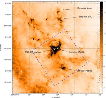
Fig. 1. Visual extinction map towards the whole Aquila Rift / Serpens region derived by us from 2MASS data (see details in Schneider et al. 2010). The spatial resolution is 20 FWHM. The dashed blue rectangle indicates the Herschel coverage. It comprises the bright HIIregion W40 (white circle), the Serpens South cluster (white star), and the HIIregion Sh2-62, associated with the young star MWC297. The Aquila Rift corresponds to the large elongated structure from the northeast to the southwest. Emisson from the Galactic plane is seen in the southeast corner.

per was used as a mapmaking algorithm. The PACS data were reduced in HIPE 3.0. We used an updated version of the cali-bration files following the most recent prescriptions of the PACS ICC (see K¨onyves et al. 2010 for details). Multiresolution me-dian and second-order deglitching, as well as a high-pass filter-ing over the full scan leg length, were applied. The final PACS maps were created using the photProject task, which performs simple projection of the data cube on the map grid.

The resulting PACS maps are displayed in Fig. 2. Owing to the rapid mapping speed, the resulting point spread functions (PSFs) are elongated in the scan directions leading to cross-like shapes of the PSFs with expected sizes of 5.900×12.200 at 70 µm and 11.600_×15.700 _{at 160 µm. The resulting rms in these} maps ranges from 50 to 1000 mJy/beam at 70 µm and from 120 to 2200 mJy/beam at 160 µm, depending on the level of back-ground in the map. It is in the W40/Sh2-64 HIIregion that the background level is the highest.

3. Overview and distance of the Aquila Rift complex

The Aquila Rift is a coherent, 5◦long feature above the Galactic plane at l=28◦_{, clearly visible on an extinction map derived} from the reddening of stars in 2MASS (Fig. 1). A distance of 225 ± 55 pc has been derived for this extinction wall, us-ing spectro-photometric studies of the optically visible stars (Straiˇzys et al. 2003). This distance is very similar to the usu-ally adopted distance of 260 ± 37 pc for the Serpens star-forming region1, located only 3◦north (Straiˇzys et al. 1996).

1 _{Note that a larger distance of 415 ± 25 pc has been recently claimed}

for Serpens Main based on a VLBA parallax of EC95, a young AeBe star embedded in Serpens Main (Dzib et al. 2010).

On the other hand, the most active and main extinction fea-ture in the 2MASS extinction map is associated with the HII region W40/Sh2-64, which has so far been considered to be at a distance ranging from 100 and 700 pc depending on au-thor (Smith et al. 1985; Vallee 1987 and references therein). These distance estimates are mostly based on kinematical dis-tances that have large uncertainties. W40 could therefore be at the same distance as Serpens. Recently, Gutermuth et al. (2008) reported Spitzer observations of an embedded cluster, referred to as Serpens South, in the Aquila Rift region. This cluster is located very close in projection on the sky to W40 (see Fig. 1) and thus seems to be part of the W40 region. Gutermuth et al. (2008) proposed that the Serpens South cluster should be part of Serpens since it has the same velocity (6 km/s). The molecu-lar cloud associated with W40 and traced by CIIrecombination lines and CO (Zeilik & Lada 1978) has a velocity ranging from 4.5 to 6.5 km/s, which is also roughly the same as Serpens. More recent N2H+ observations of the entire W40/Serpens South re-gion confirm similar velocities in the whole rere-gion with velocity differences of only ∼ 2 km/s (Maury et al. in prep). It is therefore more straightforward to consider that the W40 region is a sin-gle complex at the same distance as Serpens. This distance also suits the MWC297/ Sh2-62 region since the young 10 Mstar MWC297 itself has an accepted distance of 250 pc (Drew et al. 1997). It is finally worth noting that the visual extinction map by Cambr´esy (1999) derived from optical star counts and only tracing the first layer of the extinction wall has exactly the same global aspect as the 2MASS extinction map of Fig. 1, suggesting that both Serpens Main and the W40/ Aquila Rift / MWC297 re-gion are associated with this extinction wall at 260 pc. We thus adopt the distance of 260 pc for the entire region in the follow-ing.

The 2MASS extinction map and the Herschel images (see Appendix for PACS images and K¨onyves et al. 2010 for SPIRE images) clearly show a massive cloud associated with W40. This cloud corresponds to G28.74+3.52 in (Zeilik & Lada 1978) and has a mass of 1.1 × 104_M

(derived from our 2MASS extinction map). The cloud associated with MWC297 is less massive (4.1 × 103_M

), and we obtain a total mass of 3.1×104Mfor the whole area covered by Herschel.

4. Results and analysis

4.1. Source detection and identification of protostars

A systematic source detection was performed on all 5 Herschel bands using getsources (Men’shchikov et al. 2010). This code uses a method based on a multiscale decomposition of the im-ages to disentangle the emission of a population of spatially co-herent sources in an optimized way in all bands simultaneously. We built a sample of the best candidate protostars for the whole field. These sources are clearly detected in all Herschel bands (high significance level), and we require a detection at the short-est Herschel wavelength, 70 µm (or 24 µm when Spitzer data were available), to distinguish YSOs from starless cores. Since the 24 and 70 µm emission should only trace warm dust from the inner regions of the YSO envelopes, these sources can be safely interpreted as protostars. The 70 µm fluxes have even been re-cently recognized as a very good tracer of protostellar luminosi-ties (Dunham et al. 2008). On the other hand, in the PDR region of W40 some extended emission from warm dust at the HII re-gion interface could contaminate this YSO detection criterium. To avoid too stringent a contamination from this extended emis-sion, we selected only sources with an FWHM size smaller than

Fig. 4. Spectral energy distributions of a newly discovered bright Class 0 (left panel) and of a weaker Class 0 object (right panel), which was previously detected with Spitzer in Gutermuth et al. (2008).

4000 at 70 µm. Also, we had to make a source detection using a large pixel size of 600_{, which is good enough for starless cores} mostly detected in the SPIRE bands but not perfect to sample the spatial resolution at 70 µm and properly disentangle possi-ble multiple protostellar sources. A more precise detection could only be achieved in a reduced area in the Serpens South region (see Sect. 4.4).

A large number of compact sources are clearly seen in the 70 µm map down to the sensitivity limit of the survey. In the whole Aquila field, 201 YSOs were detected with getsources. The best achieved rms (50 mJy/beam) in the Aquila 70 µm map in the lowest background regions corresponds to a 5 σ detec-tion level in terms of protostar luminosity of 0.05 Lusing the Dunham et al. (2008) relationship. In contrast, in the highest background regions, the 5 σ detection level is then as high as 1.0 L. To account for the variable background level in Aquila, we performed simulations to evaluate the final completeness level of the YSO detection and obtained a 90 % completeness level of ∼0.2 L(see K¨onyves et al. 2010), which is compatible with the above rough estimates using Dunham et al. (2008).

4.2. Spatial distribution of the protostars

We plotted in Fig. 3 the spatial distribution of the Herschel sam-ple of 201 YSOs overlaid on the map of the dust temperature derived from a simple graybody fit of the Herschel data (see de-tails in K¨onyves et al. 2010). It is clear that the W40 region cor-responds to the most active star-forming region in the Herschel coverage with 90 % of the detected protostars. A second, much less rich, site corresponds to MWC297 with 8 % of the proto-stars, and another site to the east of W40 can be tentatively iden-tified with very few candidate protostars.

4.3. Basic properties of the protostars: Menvand Lbol

For each source an SED was built using the 5 bands of Herschel, as well as Spitzer photometry (Gutermuth et al. 2008) and MAMBO 1.2mm data (Maury et al. in prep) when available. These SEDs were systematically fitted using graybody functions to derive Menvin a systematic way, while the basic properties Lbol, Lλ>350submm, and Tbol were obtained by simple integrations of the SEDs. Two representative SEDs are displayed in Fig. 4 with a newly discovered Class 0 object and a weaker Class 0 source, which has a Spitzer counterpart in Gutermuth et al. (2008).

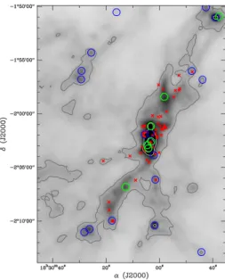
Fig. 5. Herschel SPIRE 350µm image of the Serpens South re-gion with the distribution of Herschel candidate protostars (blue circles) from the whole field extraction, of the 7 newly discov-ered Class 0 protostars (green circles), and of the Spitzer YSOs (red crosses; Gutermuth et al. 2008).

4.4. A close-up view of the Serpens South region

To go one step further in the identification and characterization of the Herschel protostars, we performed a more detailed analy-sis of the sources in a small area around the Serpens South clus-ter. In this area, we made a dedicated getsources source extrac-tion using a smaller size pixel of 300, and we could compare these first results with the Spitzer protostar population by Gutermuth et al. (2008). We used getsources on 8 bands from 8 to 1200 µm by adding the 8 and 24 µm Spitzer and the 1.2mm MAMBO data to the 5 Herschel bands.

A synthesized view of these first results based on this novel panchromatic analysis of infrared to millimeter range data for this area is given in Fig. 5. It shows the distribution of Herschel protostars compared to the Spitzer sources. The first analysis of this field indicates that even in a highly clustered region like Serpens South, a significant population of protostars were found to be missing by pure near and mid-infrared imaging with as many as 7 newly detected Class 0 objects in this field. We also

note that the Spitzer protostars (most of these not detected with Herschel) probably correspond to evolved or low-luminosity Class I objects.

5. Global view of the protostellar population in Aquila

Using the basic properties derived in Sect. 4.3, we can draw the first picture of the property space Herschel is going to cover thanks to its unprecedentedly sensitive and high spatial resolu-tion in the far-infrared.

In Fig. 6 we plotted the location of the 201 Herschel YSOs obtained in the entire field in a Menv− Lbolevolutionary diagram used to compare observed properties with theoretical evolution-ary models or tracks. The displayed tracks represent the expected evolution of protostars of masses 0.2, 0.6, 2.0, and 8.0 Mfrom the earliest times of accretion (upper left part of the diagram) to the time of 50 % mass accreted (conceptual limit between Class 0 and Class I YSOs), and the time for 90 % mass accreted (see Bontemps et al. 1996; Saraceno et al. 1996; Andr´e et al. 2000; Andr´e et al. 2008). In this plot, we distinguished objects with an Lλ>350_submm/L70−500_bol higher than 0.03 which could be safely recognized as Class 0 objects, from YSOs with Lλ>350_submm/L70−500

bol lower than 0.01 which are proposed to be Class I sources. The in-termediate objects with 0.03 > Lλ>350_submm/L70−500

bol > 0.01 should be seen as objects with an uncertain classification. A forthcoming analysis will resolve their nature by building complete SEDs in-cluding Spitzer data for a large part of the Aquila field. So far we could safely classify objects only in the reduced area of Serpens South (Sect. 4.4). In this subfield, we verified that objects with Lλ>350_submm/L70−500_bol > 0.03 and T_bol70−500 < 27 K using the reduced (only the 5 Herschel bands from 70 to 500 µm) SED coverage are indeed all found to be Class 0 objects based on the full cov-erage from 8 µm to 1.2 mm. We see that the obtained location of Class 0 and Class I YSOs is compatible with the 50 % mass accreted limit. Imposing Class 0 objects to have to be above this limit (dashed line in Fig. 6), we finally found between 45 (for T_bol70−500< 27 K) and 60 (Lλ>350_submm/L70−500_bol > 0.03) Class 0 objects in the entire field of Aquila.

In conclusion, even if the precise locations of the Herschel protostars in this diagram are seen as a preliminary result and will be updated with a more complete analysis and source detec-tion, our early results clearly indicate that Herschel is a power-ful tool for probing the virtually unexplored area of the physical properties of the earliest stages of protostellar evolution.

Acknowledgements. SPIRE has been developed by a consortium of institutes led by Cardiff Univ. (UK) and including Univ. Lethbridge (Canada); NAOC (China); CEA, LAM (France); IFSI, Univ. Padua (Italy); IAC (Spain); Stockholm Observatory (Sweden); Imperial College London, RAL, UCL-MSSL, UKATC, Univ. Sussex (UK); Caltech, JPL, NHSC, Univ. Colorado (USA). This develop-ment has been supported by national funding agencies: CSA (Canada); NAOC (China); CEA, CNES, CNRS (France); ASI (Italy); MCINN (Spain); SNSB (Sweden); STFC (UK); and NASA (USA). PACS has been developed by a con-sortium of institutes led by MPE (Germany) and including UVIE (Austria); KUL, CSL, IMEC (Belgium); CEA, LAM (France); MPIA (Germany); IFSI, OAP/AOT, OAA/CAISMI, LENS, SISSA (Italy); IAC (Spain). This develop-ment has been supported by the funding agencies BMVIT (Austria), ESA-PRODEX (Belgium), CEA/CNES (France), DLR (Germany), ASI (Italy), and CICT/MCT (Spain). We thanks Rob Gutermuth for providing us with the list of Spitzer sources in the Serpens South sub-field prior to publication.

References

Allen, L., Megeath, S. T., Gutermuth, R., et al. 2007, Protostars and Planets V, 361

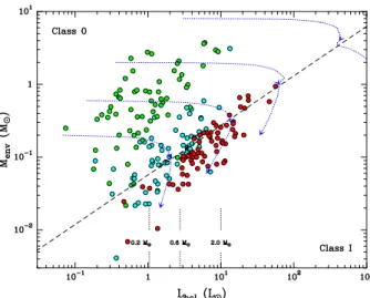
Fig. 6. Distribution of the Herschel sample of protostars in the protostellar evolutionary diagram Menv − Lbol. The green and red circles are for the Class 0 and Class I protostars with Lλ>350_submm/L70−500

bol > 0.03 and < 0.01 (see text), respec-tively. The intermediate, more uncertain cases with 0.03 > Lλ>350_submm/L70−500_bol > 0.01 are displayed as light blue circles. The evolutionary tracks for 0.2, 0.6, 2.0, and 8.0 M are displayed as dotted curves. The formal separation between Classes 0 and I in this diagram corresponds to 50 % of the mass accreted, which corresponds to the locii of the first arrows on the curves (see also the dashed separating line). The second arrows on the curves in-dicate 90 % of the mass accreted.

Andr´e, P., Men’shchikov, A., Bontemps, S., et al. 2010, A&A, this volume Andr´e, P., Minier, V., Gallais, P., et al. 2008, A&A, 490, L27

Andr´e, P., Ward-Thompson, D., & Barsony, M. 2000, Protostars and Planets IV, 59

Bontemps, S., Andr´e, P., Kaas, A. A., et al. 2001, A&A, 372, 173 Bontemps, S., Andr´e, P., Terebey, S., & Cabrit, S. 1996, A&A, 311, 858 Cambr´esy, L. 1999, A&A, 345, 965

Di Francesco, J., Evans, II, N. J., Caselli, P., et al. 2007, in Protostars and Planets V, ed. B. Reipurth, D. Jewitt, & K. Keil, 17–32

Drew, J. E., Busfield, G., Hoare, M. G., et al. 1997, MNRAS, 286, 538 Dunham, M. M., Crapsi, A., Evans, II, N. J., et al. 2008, ApJS, 179, 249 Dzib, S., Loinard, L., Mioduszewski, A. J., et al. 2010, ArXiv:1003.5900 Evans, N. J., Dunham, M. M., Jørgensen, J. K., et al. 2009, ApJS, 181, 321 Griffin, M. et al. 2010, A&A, this volume

Gutermuth, R. A., Bourke, T. L., Allen, L. E., et al. 2008, ApJ, 673, L151 Kaas, A. A., Olofsson, G., Bontemps, S., et al. 2004, A&A, 421, 623 K¨onyves, V., Andr´e, P., Men’shchikov, A., et al. 2010, A&A, this volume Men’shchikov, A., Andr´e, P., Didelon, P., et al. 2010, A&A, this volume Nordh, L., Olofsson, G., Abergel, A., et al. 1996, A&A, 315, L185 Pilbratt, G. et al. 2010, A&A, this volume

Poglitsch, G. et al. 2010, A&A, this volume

Saraceno, P., Andr´e, P., Ceccarelli, C., Griffin, M., & Molinari, S. 1996, A&A, 309, 827

Schneider, N., Bontemps, S., Simon, R., et al. 2010, ArXiv:1001.2453 Smith, J., Bentley, A., Castelaz, M., et al. 1985, ApJ, 291, 571 Straiˇzys, V., ˇCernis, K., & Bartaˇsi¯ut˙e, S. 1996, Baltic Astronomy, 5, 125 Straiˇzys, V., ˇCernis, K., & Bartaˇsi¯ut˙e, S. 2003, A&A, 405, 585 Swinyard, B. M., Ade, P., Baluteau, J. P., et al. 2010, A&A, this volume Vallee, J. P. 1987, A&A, 178, 237

1 _{Laboratoire AIM, CEA/DSM–CNRS–Universit´e Paris Diderot,}

IRFU/Service d’Astrophysique, C.E. Saclay, Orme des Merisiers, 91191 Gif-sur-Yvette, France

2 _{CNRS/INSU, Laboratoire d’Astrophysique de Bordeaux, UMR}

5804, BP 89, 33271 Floirac cedex, France

3 _{Universit´e de Bordeaux, OASU, Bordeaux, France}

4 _{European Southern Observatory, Karl Schwarzschild Str. 2, 85748}

Garching, Germany

5 _{INAF-IFSI, Fosso del Cavaliere 100, 00133 Roma, Italy} 6 _{IAS, CNRS-INSU–Universit´e Paris-Sud, 91435 Orsay, France} 7 _{Laboratoire d’Astrophysique de Marseille, CNRS/INSU–Universit´e}

de Provence, 13388 Marseille cedex 13, France

8 _{CESR & UMR 5187 du CNRS/Universit´e de Toulouse, BP 4346,}

31028 Toulouse Cedex 4, France

9 _{Observatoire astronomique de Strasbourg, UMR 7550}

CNRS/Universit´e de Strasbourg, 11 rue de l’Universit´e, 67000, Strasbourg

10 _{IRAM, 300 rue de la Piscine, Domaine Universitaire, 38406 Saint}

Martin d’H`eres, France

11 _{National Research Council of Canada, Herzberg Institute of}

Astrophysics, University of Victoria, Department of Physics and Astronomy, Victoria, Canada

12 _{School of Physics and Astronomy, Cardiff University, Queens}

Buildings The Parade, Cardiff CF24 3AA, UK

13 _{National Astronomical Observatories, Chinese Academy of}

Sciences, Beijing 100012, China

14 _{CITA & Dep. of Astronomy and Astrophysics, University Toronto,}

Toronto, Canada

15 _{Herschel Science Center, ESAC, ESA, PO Box 78, Villanueva de la}

Ca˜nada, 28691 Madrid, Spain

16 _{Department of Astronomy, Stockholm Observatoty, AlbaNova}

University Center, Roslagstullsbacken 21, 10691 Stockholm, Sweden

17 _{Institut d’Astrophysique de Paris, UMR7095 CNRS, Universit}

Pierre et Marie Curie, 98 bis Boulevard Arago, 75014 Paris, France

18 _{Astronomy Technology Centre, Royal Observatory Edinburgh,}

Blackford Hill, EH9 3HJ, UK

19 _{INAF–Osservatorio Astrofisico di Arcetri, Largo Fermi 5, 50125}

Firenze, Italy

20 _{Science and Technology Facilities Council, Rutherford Appleton}

Laboratory, Chilton, Didcot OX11 0NL, UK

21 _{Department of Physics & Astronomy, The Open University, Walton}

Hall, Milton Keynes MK7 6AA, UK

22 _{Department of Physics and Astronomy, McMaster University,}

Hamilton, ON L8S 4M1, Canada

23 _{SUPA, Institute for Astronomy, Edinburgh University, Blackford}

Fig. 2. PACS 70 µm (left) and 160 µm (right) images of the Aquila field. See details about data reduction and map making in Sect. 2 and in K¨onyves et al. (2010). The corresponding SPIRE 250, 350, and 500 µm images are shown in K¨onyves et al. (2010).

Fig. 3. Distribution map of the 201 Herschel YSOs selected in Sect. 4.1, over-plotted on the map of dust temperature. The dust temperature map was derived from graybody fits to the Herschel data (see details in K¨onyves et al. 2010).