Characterization of lube oil derived diesel engine particulate emission rate vs. lube oil consumption

Characterization of Lube Oil Derived Diesel Engine Particulate Emission Rate vs. Lube Oil Consumption

by

Thomas C. Miller

Bachelor of Science in Naval Architecture and Marine Engineering United States Coast Guard Academy, 1989

Submitted to the Department of Ocean Engineering and the Department of Mechanical Engineering in Partial Fulfillment of the Requirements for the Degrees of

Master of Science in Naval Architecture and Marine Engineering and

Master of Science in Mechanical Engineering at the

Massachusetts Institute of Technology May 1996

© Thomas C. Miller, 1996. All Rights Reserved.

The Author hereby grants MIT and the U.S. Government permission to reproduce and distribute copies of this thsis document in whole oip part

Signature of Author

Certified by

Dr. Alan J. Brown Professor, Department of Ocean Engineering

Thesis Advisor Certified by

. Victor W. Wong Lecturer, Department of Mechanical Engineering

Thesis Advisor

Accepted by . -.

--- a-· e -- A. Douglas Carmichael Chairman, Departmental Graduate Committee

DepartmentofIQeQan Engineering Accepted by

uL~-r - ~ A. A. Sonin Chairman, Departmental Graduate Committee

Department of Mechanical Engineering MASSACHUSETTS INSTITUTE

Characterization of Lube Oil Derived Diesel Engine Particulate Emission Rate vs.

Lube Oil Consumption

by

Thomas C. Miller

Submitted to the Departments of Ocean Engineering and Mechanical Engineering on May 10, 1996 in Partial Fulfillment of the Requirements for the Degrees of

Masters of Science in Naval Architecture and Marine Engineering and

Masters of Science in Mechanical Engineering ABSTRACT

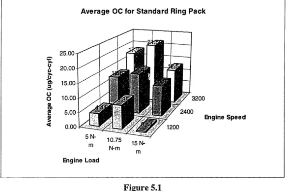
The primary focus of this study is the evaluation of oil consumption and lube oil derived particulate emission rate characteristics for a direct injection diesel engine. Ring pack configurations, air intake manifold pressures, engine speed and engine load were varied to obtain a general cause-and-effect relation. A Real Time Oil Consumption (RTOC) Sulfur Dioxide-based measurement technique was used to measure oil consumption (OC). A scaled down version of the EPA Constant Volume Sampling System was used to measure the total particulate emission rate (TPR). The dilution tunnel used by Laurence [2] was modified to dilute the entire exhaust flow as opposed to only a fraction. Three ring pack and three air intake manifold pressure configurations were studied during steady state operation, at three varied speeds and loads, in an effort to 1) validate the relationship between OC and the particulate emissions, and 2) develop an empirical correlation between the OC and the lube oil derived TPR. Four tests were conducted for each speed and load combination and air intake pressure for ring pack one and for ring pack two for two speeds and loads (total of 98 particulate samples). Two tests were run for ring pack three at two speeds and loads (total of 8 particulate samples). Each particulate sample was collected on a 47mm teflon coated glass fiber filter and analyzed via a soxlet extraction method [ORTECH] for determination of the soluble organic fraction (SOF). Further analysis was conducted of specific samples for determination of the lube oil contribution to the SOF.

A secondary study was also completed in conjunction with the above which evaluated comparisons between a portable Gaseous Emissions Detector ENERAC 2000ET M

, which utilizes electrochemical sensors, and the MIT Gas Cart, which utilizes a combination of infrared, polarographic and chemiluminesent sensors, to identify the relativistic trends of the two machines. Good correlation between the two apparatus will assist the Coast Guard's effort to validate the use of electrochemical sensors for monitoring mobile sources of gaseous emissions.

Thesis Advisor: Alan J. Brown

Title: Professor, Department of Ocean Engineering Thesis Supervisor: Victor W. Wong

DEDICATION

The completion of this document is dedicated to five very important people in my life. First, to my Grandmother, the late Margaret Miller. A true Academe in every sense of the word who passed away during the spring of 1995. She would truly have enjoyed seeing the evolution and completion of this thesis and my graduation from such a prestigious institution.

To my Mom and Dad, who instilled in me over the years the character, drive, and dedication that my Coast Guard career requires, this Institution demands, and that my family life will strive and grow with for years to come. Thank you!

To my wife, Gail, you have been my inspiration since February 22, 1989. I would not have believed it if I had not experienced it, but as it has been said, "Behind every man is a great woman." I'm everything I am because of you! Your support, encouragement, sense of humor and love made this advanced world of study bearable.

Finally, to my daughter Annie who'was born July 25, 1995 during the final summer term at MIT. You have truly made my life sparkle. Although your too young to understand what is happening, you unknowingly provided a daily reality check that allowed me to leave the rigors of work behind and to enjoy the truly important things in life.

ACKNOWLEDGEMENTS

The completion of this thesis would not have been possible without the help of many different people. First, to the faculties and staffs of the Ocean Engineering and Mechanical Engineering Departments and the Sloan Automotive Laboratory. The education I received from you at this Institution goes far beyond any classroom lecture. You have provided me with the knowledge and resources a sound Engineer needs to practically approach and solve engineering problems with confidence. I am certain that I will be afforded the opportunity to employ this newly acquired expertise during my Coast Guard Career and future endeavors. I thank you.

To Captain Alan Brown and Dr. Victor Wong, I truly appreciate the patience, guidance and time that you both afforded me during the completion of this academic milestone. Thank you. Also special thanks to Professor John Heywood for providing an invaluable reference.

To Nancy Cook and Brian Corkum of the Sloan Automotive Laboratory Staff, you two are invaluable resources within this lab! Nancy, your administrative expertise and EREQ assistance made my life so much easier. Brian, your patience and willingness to teach is unsurpassed. You taught me a great deal about diesel engine operation and practical engineering which is greatly appreciated. Thank you to you both.

To my Coast Guard Colleagues:

To Lee Boone. Lee, I could not have completed these two years of study without you. Thanks for sharing in the "Odd" miseries of MIT, the rigors of academe, and the subtle niceties of the Muddy. See you in D.C.

To Mark Jackson, it was truly a rewarding experience working with you throughout our thesis work. I feel very fortunate to have been a member of this research team, and really appreciate your flexibility and understanding when my February schedule changed so abruptly. Thanks, I could not have competed this research without you. From the future Commander of the USCGC Big Brown Desk, I wish you Fair Winds and Following Seas. Good Luck!

To the Coast Guard Officers who came before me, Dan Pippenger, Rob Wilcox, Doug Schofield, and Eric Ford, thanks for showing me the way.

To all the Navy Officers, Tom Moore, Bob Meyer, Chris Trost. Tim McCue and others, its been a pleasure. Good Luck.

To the Sloan Laboratory Researchers, Mark Kiesel, Alan Shihadeh, Bouke Noordzij, and Tian Tian, it has been a pleasure working with you. Good Luck in your future endeavors.

Special thanks to ORTECH Corporation, specifically, John Lopatynski for the efficient and professional laboratory analysis you conducted. You provided timely assistance and that is greatly appreciated.

This project was primarily sponsored by the Maritime Administration (MARAD) with support from the United States Coast Guard (USCG) under contract DTMA 91-95-00051. Special thanks to Dan Leubecker of MARAD and Dr. Alan Bentz of the USCG Research and Development Center for their guidance and support. This project is also supported by the Consortium of Lubrication in Internal Combustion Engines, whose members include Dana Corporation, Peugeot, Renault, and Shell Oil

Table of Contents Abstract Dedication Acknowledgments Table of Contents List of Abbreviations List of Figures List of Tables Chapter 1 -Chapter 2 -Chapter 3 -Chapter 4 -Chapter 5 -Chapter 6 -Chapter 7 -Appendix I Appendix II Appendix III -Introduction Motivation Experimental Set Up Calculations

Results and Analysis

Conclusions and Recommendations References

Specific OC Data Std. Ring Pack

Std. Ring Pack: Varied Intake Press. Varied RP (1200 RPM-Low Load) Varied RP (1200 RPM-Med Load) Varied RP (2400 RPM-Low Load) Varied RP (2400 RPM-Med Load) Particulate Rate Data

Raw Particulate Data L/O SOF vs. OC

Std. Ring Pack (1200 RPM)

Std. Ring Pack: Varied Intake Press. Std. Ring Pack (2400 RPM)

Std. Ring Pack (3200 RPM) Varied RP (1200 RPM-Low Load) Varied RP (1200 RPM-Med Load) Varied RP (2400 RPM-Low Load) Varied RP (2400 RPM-Med Load) L/O SOF vs. OC

Calibration Curves for Emission Analyzers Volumetric Flow Meter Calib. MIT Gas Cart Calibration Curves

CO2 CO NO Section Page # 3 5 7 9 13 16 19 21 23 26 50 59 95 103 105 106 107 108 109 110 111 113 114 116 117 118 119 120 121 122 123 124 126 127 128 129 130

Table of Contents

Appendix III

Appendix IV

Calibration Curves for Emission Analyzers (Continued)

NO, 131

02 132

ENERAC 2000ETM _{Calibration Curves}

CO 133

NO 134

NOX 135

02 136

Sensor Comparison Curves. 138

Steady State Operating Conditions:

CO2: 1200 RPM 5 N-m 139 CO: 1200 RPM 5 N-m 140 NO: 1200 RPM @ 5 N-m 141 NO,: 1200 RPM @ 5 N-m 142 CO2: 1200 RPM @ 10.75 N-m 143 CO: 1200 RPM 10.75 N-m 144 NO: 1200 RPM 10.75 N-m 145 NO,: 1200 RPM 10.75 N-m 146 CO2: 1200 RPM @ 15 N-m 147 NO: 1200 RPM @ 15 N-m 148 NO,: 1200 RPM @ 15 N-m 149 CO2: 2400 RPM 5 N-m 150 CO: 2400 RPM @ 5 N-m 151 NO: 2400 RPM @ 5 N-m 152 NO,: 2400 RPM@5 N-m 153 CO2: 2400 RPM 10.75 N-m 154 CO: 2400 RPM 10.75 N-m 155 NO: 2400 RPM 10.75 N-m 156 NO,: 2400 RPM 10.75 N-m 157 CO2: 2400 RPM @ 15 N-m 158 CO: 2400 RPM @ 15 N-m 159 NO: 2400 RPM @ 15 N-m 160 NO,: 2400RPM @ 15 N-m 161 CO₂: 3200 RPM @ 5 N-m 162 CO: 3200 RPM 5 N-m 163 NO: 3200 RPM @ 5 N-m 164 NO,: 3200 RPM @ 5 N-m 165 CO₂: 3200 RPM @ 10.75 N-m 166 CO: 3200 RPM 10.75 N-m 167 NO: 3200 RPM 10.75 N-m 168 NO,: 3200 RPM @ 10.75 N-m 169 Section Page #

Table of Contents

Section Pa~~~~~~~~~~~~~~~~~~~~~~~~~~~~~~~~~~~~~~~~~~~ne

Appendix IV

Appendix V

Sensor Comparison Curves (Continued) Steady State Operating Conditions: CO,: 3200 RPM @ 15 N-m NO: 3200 RPM @ 15 N-m NOx: 3200 RPM @ 15 N-m

Load Transient Operating Conditions: CO2: 5 to 10.75 N-m; 2400 RPM CO: 5 to 10.75 N-m; 2400 RPM

NO: 5 to 10.75 N-m; 2400 RPM

NOx: 5 to 10.75 N-m; 2400 RPM Speed Transient Operating Conditions: CO2: 3200 to 2400 RPM; 5 N-m CO: 3200 to 2400 RPM; 5 N-m NO: 3200 to 2400 RPM; 5 N-m NOx: 3200 to 2400 RPM; 5 N-m Gaseous Emission Data

170 171 172 173 174 175 176 177 178 179 180 182 Section

Page #

List of Abbreviations Abbreviation Meaning MIT OC RTOC TPR EPA GC MS SOF Non-SOF mm MARAD TPM CO

Co,

Massachusetts Inst. of Technology Oil Consumption

Real Time Oil Consumption Total Particulate Rate

Environmental Protection Agency Gas Chromatography

Mass Specification Soluble Organic Fraction Insoluble Organic Fraction Millimeter

Maritime Administration Total Particulate Matter Carbon Monoxide Carbon Dioxide Oxygen Nitric Oxide Nitrogen Dioxide Nitrogen Hydrogen Sulfur Dioxide

Revolutions Per Minute Revolutions Per Second Minute

Number of Cylinders Mass Flow Rate of Exhaust Mass Flow Rate of Intake Air Volumetric Flow Rate of Fuel Fuel Density

Weight of Water in Air

Weight fraction of Water in Air

Molar Concentration due to Combustion Exhaust Content as a Weight Percent Hydrogen to Carbon Fuel Ratio C02 Concentration in Exhaust CO Concentration in Exhaust Actual Air to Fuel Ratio

# of Carbon Atoms / Fuel Molecule # of Hydrogen Atoms / Fuel Molecule Molecular Weight of the Exhaust

mg/cyl/cycle mg/cyl/cycle Percentage Percentage grams Rev/min Rev/sec Minute cm3/min kg/m3 Percent Percent Percent Percent Percent Percent kilogram Units

Abreiaio M U

S02 Exhaust Flow Rate

Output of Detector With Sample Output of Detector With Span Gas S02 Concentration in Span Gas

Sulfur Content in Fuel Oil Sulfur Content in Lube Oil

Output Voltage of Cell Air Detector # of Cycles per Revolution

Total Sample Mass Final Filter Mass Initial Filter Mass Dilution Ratio Sample Density Ambient Air Density Exhaust Density

Mass Flow Rate of Sample Volumetric Flow Rate of Sample Total Sample Time

Total Particulate Mass

International Standards of Operation Standard Ring Pack

Varied Ring Packs Fuel to Air Ratio Sexhaust Sample,,lt Spanvolt Spanppm Fuelppm Lubeppm Airvolt nr msampletotal mfinal minitial rd Psample Pair Pexhaust Qsample Vsample tsample mparticulate ISO SRP VRP F/A volts volts ppm ppm ppm volts cyc/rev grams grams grams kg/m3 kg/m3 kg/m3 kg/sec liter/sec sec grams

List of Figures

Figure Description Page #

2.1 Relation Between OC and Oil Derived Particulate 24

3.1 OC Sampling System 28

3.2 Particulate Formation Process 30

3.3 Particuiate Sampling System 34

3.4 Test Matrix Labeling System 38

3.5 Oil Consumption @ 1200 RPM-Low Load 41

3.6 Oil Consumption @ 1200 RPM- Medium Load 41

3.7 ENERAC 2000ETM Set Up 47

3.8 MIT Gas Cart Set Up 48

4.1 OC Calculation Flow Chart 50

4.2 Particulate Rate Calculation Flow Chart 56

5.1 OC Comparison Between Test Conditions 59

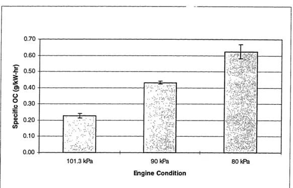
5.2 Specific OC Trends for Std. Ring Pack 60

5.3 Specific OC Trends for SRP w/ Varied Intake Press. 61

5.4 Specific OC Trends Between RP (1200 RPM-Low) 62

5.5 TPR Comparison (2400/200 RPM-Varied Load) 63

5.6 TPR Composition (1200 RPM: Varied Intake Air Press.) 64

5.7 Validity Comparison with Laurence 67

5.8 Specific Oil Derived SOF vs. OC 70

5.9 Specific Oil Derived SOF vs. Engine Condition 71

5.10 Particulate Rate & L/O SOF Comparison 72

5.11 L/O SOF Percent of Engine OC 73

5.12 L/O SOF Percent of Engine OC: Varied Intake Air Press. 74 5.13 L/O SOF vs. OC; RP Comparison (1200 RPM-Low Load) 75 5.14 L/O SOF vs. OC; RP Comparison (2400 RPM-Low Load) 75

5.15 CO2Dependence On 02 Concentration 78

5.16 CO2 Sensor Repeatability @ 3200 RPM-Medium Load 79

5.17 Average CO2Readout @ 3200 RPM-Medium Load 79

5.18 CO2 Sensor Response to Load Transient 80

5.19 CO2 Sensor Response to Speed Transient 80

5.20 CO Sensor Repeatability @ 3200 RPM-Medium Load 82

5.21 Average CO Readout @ 3200 RPM-Medium Load 83

5.22 CO Sensor Response to Load Transient 83

5.23 CO Sensor Response to Speed Transient 84

5.24 NO Sensor Repeatability @ 3200 RPM-Medium Load 85

5.25 Average NO Readout @ 3200 RPM-Medium Load 86

5.26 NO Sensor Response to Load Transient 86

5.27 NO Sensor Response to Speed Transient 87

List of Figures (Continued)

Pae #

@

Average NO, Readout ( 3200 RPM-Medium Load NO Sensor Response to Load Transient

NO Sensor Response to Speed Transient

02 Sensor Repeatability

@

@

Specific OC for Specific OC for Specific OC for Specific OC for Specific OC for Specific OC for

Standard Ring Pack

Standard Ring Pack: Varied Intake Press. Varied Ring Packs

Varied Ring Packs Varied Ring Packs Varied Ring Packs

(1200 (1200 (2400 (2400 Specific L/O SOF vs. Specific OC: SRP, 1 Specific L/O SOF vs. Specific OC: SRP, ' Specific L/O SOF vs. Specific OC: SRP, 2 Specific L/O SOF vs. Specific OC: SRP, 3 Specific L/O SOF vs. Specific OC: VRP, Specific L/O SOF vs. Specific OC: VRP, I Specific L/O SOF vs. Specific OC: VRP, Specific L/O SOF vs. Specific OC: VRP,, Specific L/O SOF vs. Specific OC: Genere Volumetric Flow Meter Calibration Curve

RPM-Low Load) RPM-Med Load) RPM-Low Load) RPM-Med Load)

200 RPM laried Itk. Press.

400 RPM 3200 RPM 1200 RPM-Low 1200 RPM-Med 2400 RPM-Low 2400 RPM-Med al Trend

CO2 Sensor Calibration Curve (Gas Cart) CO Sensor Calibration Curve (Gas Cart) NO Sensor Calibration Curve (Gas Cart) NOx Sensor Calibration Curve (Gas Cart)

02 Sensor Calibration Curve (Gas Cart) CO Sensor Calibration Curve (ENERAC) NO Sensor Calibration Curve (ENERAC) NO Sensor Calibration Curve (ENERAC)

02 Sensor Calibration Curve (ENERAC) Sensor Comparison Sensor Comparison Sensor Comparison Sensor Comparison Sensor Comparison Sensor Comparison Sensor Comparison Sensor Comparison Sensor Comparison

(CO2) 1200 RPM-Low Load (CO) 1200 RPM-Low Load (NO) 1200 RPM-Low Load (NO,) 1200 RPM-Low Load (CO2) 1200 RPM-Med Load (CO) 1200 RPM-Med Load (NO) 1200 RPM-Med Load (NO,) 1200 RPM-Med Load (COD 1200 RPM-High Load

90 90 91 91 93 93 95 106 107 108 109 110 111 116 117 118 119 120 121 122 123 124 127 128 129 130 131 132 133 134 135 136 139 140 141 142 143 144 145 146 147 Figure Descrintion 5.29 5.30 5.31 5.32 5.33 5.34 5.35 A-I-i A-I-2 A-I-3 A-I-4 A-I-5 A-I-6 A-II-2 A-II-3 A-II-4 A-II-5 A-II-6 A-II-7 A-II-8 A-II-9 A-II-10 A-III-1 A-III-2 A-III-3 A-III-4 A-III-5 A-III-6 A-III-7 A-III-8 A-III-9 A-III- 10 A-IV-1 A-IV-2 A-IV-3 A-IV-4 A-IV-5 A-IV-6 A-IV-7 A-IV-8 A-IV-9 - --- -

-List of Figures (Continued) Descrintion

Sensor Comparison (NO) 1200 RPM-High Load Sensor Comparison (NO) 1200 RPM-High Load Sensor Comparison (CO2) 2400 RPM-Low Load Sensor Comparison (CO) 2400 RPM-Low Load Sensor Comparison (NO) 2400 RPM-Low Load Sensor Comparison (NO) 2400 RPM-Low Load Sensor Comparison (CO2) 2400 RPM-Med Load Sensor Comparison (CO) 2400 RPM-Med Load Sensor Comparison (NO) 2400 RPM-Med Load Sensor Comparison (NOx) 2400 RPM-Med Load Sensor Comparison (CO2) 2400 RPM-High Load Sensor Comparison (CO) 2400 RPM-High Load Sensor Comparison (NO) 2400 RPM-High Load Sensor Comparison (NOx) 2400 RPM-High Load Sensor Comparison (CO2) 3200 RPM-Low Load Sensor Comparison (CO) 3200 RPM-Low Load Sensor Comparison (NO) 3200 RPM-Low Load Sensor Comparison (NO) 3200 RPM-Low Load Sensor Comparison (CO2) 3200 RPM-Med Load Sensor Comparison (CO) 3200 RPM-Med Load Sensor Comparison (NO) 3200 RPM-Med Load Sensor Comparison (NOx) 3200 RPM-Med Load Sensor Comparison (CO2) 3200 RPM-High Load Sensor Comparison (NO) 3200 RPM-High Load Sensor Comparison (NO) 3200 RPM-High Load Sensor Comparison (CO2) Load Trans: 2400 RPM, L-M Sensor Comparison (CO) Load Trans: 2400 RPM, L-M Sensor Comparison (NO) Load Trans: 2400 RPM, L-M Sensor Comparison (NO) Load Trans: 2400 RPM, L-M Sensor Comparison (CO2) Speed Transt: 3200-2400, Low Sensor Comparison (CO) Speed Transt: 3200-2400, Low Sensor Comparison (NO) Speed Trans: 3200-2400, Low Sensor Comparison (NO) Speed Trans: 3200-2400, Low

Figure Page # A-IV-10 A-IV- 11 A-IV-12 A.,IV-13 A-IV-14 A-IV-15 A-IV-16 A-IV-17 A-IV-18 A-IV-19 A-IV-20 A-IV-21 A-IV-22 A-IV-23 A-IV-24 A-IV-25 A-IV-26 A-IV-27 A-IV-28 A-IV-29 A-IV-30 A-IV-31 A-IV-32 A-IV-33 A-IV-34 A-IV-35 A-IV-36 A-IV-37 A-IV-38 A-IV-39 A-IV-40 A-IV-41 A-IV-42 148 149 150 151 152 153 154 155 156 157 158 159 160 161 162 163 164 165 166 167 168 169 170 171 172 173 174 175 176 177 178 179 180

List of Tables

Table Description Page #

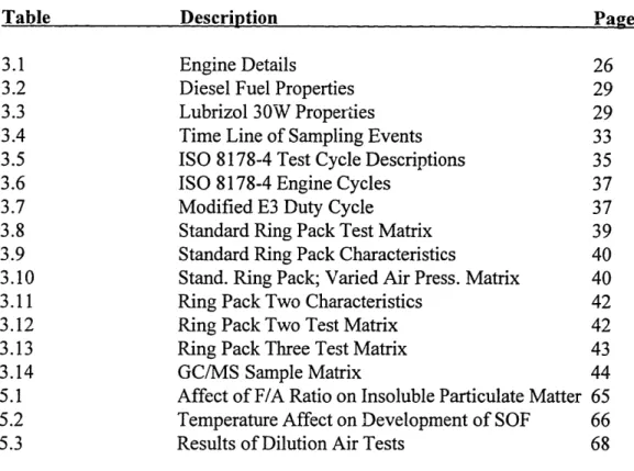
3.1 Engine Details 26

3.2 Diesel Fuel Properties 29

3.3 Lubrizol 30W Properties 29

3.4 Time Line of Sampling Events 33

3.5 ISO 8178-4 Test Cycle Descriptions 35

3.6 ISO 8178-4 Engine Cycles 37

3.7 Modified E3 Duty Cycle 37

3.8 Standard Ring Pack Test Matrix 39

3.9 Standard Ring Pack Characteristics 40

3.10 Stand. Ring Pack; Varied Air Press. Matrix 40

3.11 Ring Pack Two Characteristics 42

3.12 Ring Pack Two Test Matrix 42

3.13 Ring Pack Three Test Matrix 43

3.14 GC/MS Sample Matrix 44

5.1 Affect of F/A Ratio on Insoluble Particulate Matter 65

5.2 Temperature Affect on Development of SOF 66

Chapter 1

INTRODUCTION

1.1 Background.

The primary motivation for this research project stems from the International Maritime Community's interest in reducing air pollution from ships, specifically, MARPOL Annex VI - "The Prevention of Air Pollution From Ships". In an effort to obtain a clear insight into the pollution characteristics of diesel engines (particularly those in marine applications), the United States Coast Guard in conjunction with the Maritime Administration (MARAD) co-sponsored the research project "Characterization and Assessment of Diesel Particulate Emissions Reduction Via Oil Consumption Control", MARAD Contract/Grant Number: DTMA91-95-H-00051.

This thesis focuses on two topics that influence the control of air pollution from ships. The primary area of study is determining the relationship between the lubricating oil derived particulate emission rate and the engine oil consumption. If such a relation does exist, then by controlling oil consumption, particulate emissions can be attenuated.

The secondary area of study attempts to provide equivalence data for the ENERAC 2000ETM portable gaseous emissions detector, which utilizes electrochemical sensors, by comparison with validated analyzers that employ infrared, polarographic and chemiluminesent sensors. The validation of this briefcase-sized detector for shipboard applications will allow for simple adaptation to any vessel for the monitoring of air pollutants emitted by engine exhaust.

1.2 Previous Works.

The reduction of particulate emissions from diesel engines has been the subject of many studies in recent years. Diesel particulate matter is a complex mixture of organic and inorganic compounds in the solid and liquid phases that can be described as any exhaust component, other than uncombined water, that collects on a filter in a dilution tunnel at a temperature < 52 C [1]. Some of the many products of incomplete combustion of the diesel fuel and engine oil absorb onto the carbonaceous material of the particulate. This fraction, which is extractable in an organic solvent, is termed the soluble organic fraction [14]. It has been shown that, dependent on the operating condition, between 30 and 80 percent of the soluble organic fraction (SOF) is derived from lubricating oil [9] and that substantial reductions of the total particulate rate (TPR) could be achieved by controlling oil consumption [12].

Studies dating back to the early 80's have shown that engine lubricant consumption contributes siginificantly to diesel exhaust particulate emissions. The problem is less severe at high loads, as most of the consumed oil is oxidized due to higher temperatures. The general observation is that the lubricant fraction of particulates is greatest at light to medium load conditions where combustion chamber temperatures are less capable of oxidizing the lubricant that finds its way into the combustion gases. Conclusions in recent reports [21] indicate that it is necessary to further reduce lube oil consumption to reach mandated diesel particulate emission levels.

It has also been shown that for boats and ships maneuvering in harbors and ports, marine engines are operated at predominantly low speed and low to medium load conditions [19] that favor the "survival" of oil particulate in the exhaust and inhibit their oxidation.

The results of these previous works indicate that the particulate rate decreases with theoretical decreases in oil consumption. This conclusion suggests that particulate rate data needs to be collected simultaneously with oil consumption data to better understand and quantify the relationship.

Chapter 2

MOTIVATION

2.1 Motivation.

Air pollution is a growing problem in today's in, :astrialized society. Movements to control this ever-increasing danger to the environment and the health of workers throughout the world have become extremely prevalent. Of particular interest are particulate emissions from diesel engines. Diesel exhaust particulate is considered a potential health hazard due to its association with some polycyclic aromatic compounds (PAC) that are present in the soluble organic fraction (SOF). The emission of some of the PACs to the environment constitute the largest group of carcinogens among environmental chemical groups [9].. Approximately 90 percent of diesel particulate encompass a size range of 0.0075 to 1.0 microns. Due to the ability of these particles to be inhaled and eventually trapped in the bronchial passages and alveoli of the lungs, particulate matter poses a very serious health concern [21].

Other studies focusing on non-cancer health effects have raised equally alarming concerns. By correlating daily weather, air pollutants and mortality in five U.S. cities, scientists have discovered that non-accidental death rates tend to rise and fall in near lockstep with daily levels of particulate (more so than with other pollutants) [29]. Confirmation of these findings make airborne particulate levels the largest known "involuntary environmental insult" to which Americans are exposed [29]. This pollutant clearly affects a wide variety of people whose livelihood links them to these possible dangers of particulate emissions. Without control of diesel particulate emissions, the potential health hazard will get much worse as diesel vehicle use continues to grow throughout the world.

These reasons alone demand that research be continued to determine means of controlling particulate emissions. The Environmental Protection Agency (EPA) has issued stringent regulatory controls, as required by the Clean Air Act, requiring severe

reductions in particulate emissions from heavy duty diesels. Specifically, a 1994 heavy duty diesel standard of 0.10 g/bhp-hr and a 1996 urban bus standard of 0.05 g/bhp-hr [21,29] were enacted. Therefore, it is imperative that the research and development of particulate emission reduction strategies be continued in order to meet these standards.

The heaviest portions of the extractable particulate material have properties very much like those of engine oil. This fact has led to the qualitative conclusion that much of the extractable portion of the particulate emissions may be derived from the consumed engine oil [30]. Therefore, particulate emissions could be effectively reduced if OC is decreased. Figure 2.1 displays the effect of oil consumption on oil derived particulate emissions for one engine operating condition [17]. The trend supports the theory that reduction of oil consumption would result in significant reductions in particulate emission.

Figure 2.1

Relationship Between OC and Oil Derived Particulate

(Reproduced from SAE 900591)

(Reproduced from SAE 900591)

60

f5o

+

This study attempts to quantitatively describe the relationship between oil consumption and the lube oil derived particulate rate by simultaneously collecting OC and TPR data. The specifics of data collection, oil consumption calculation, and particulate rate calculation are described in Chapters 3 and 4.

The second portion of this study focuses on the comparison of gaseous emissions results of two measurement systems, the ENERAC 2000ETM _{and the MIT Gas Cart, in an}

effort to validate the use of the ENERAC, a briefcase-sized electrochemical sensing unit. The ENERAC was originally designed for monitoring emissions from stationary land based sources. Recent studies have attempted to gain EPA recognition, for shipboard use, by demonstrating that the portable analyzers results are comparable to much larger, rack mounted devices used on shore, and the multiple instruments used by Lloyd's Register aboard ship. The increasingly stringent emission standards demand the testing of ship emissions to determine the magnitude of emission problems and the monitoring of the effects of reduction strategies [20]. Shipboard application of emissions monitoring equipment will always be space limited and could therefore be very costly if modification is required to accommodate the equipment. For these reasons, it is important that the device be compact to limit any potential impact on the operation of the vessel thereby making the ENERAC an ideal choice. To this end, additional equivalence data must be collected from other methods of analysis to validate the shipboard application of the ENERAC 2000ETM _.

Chapter 3

EXPERIMENTAL SET UP

3.1 Test Bed.

An experimental Ricardo Hydra single cylinder, direct injection, naturally aspirated diesel engine, developed by Cussons Technology, was utilized as the test bed for this research project. The engine specifics are listed in Table 3.1.

Standard D1 Hydra 80.26 mm

Stroke: 88.90 mm

# Cylinders: 1

Swept Volume: .4498 liters

Compression Ratio: 19.8:1

Aspiration: Natural

Rated Speed: 4500 RPM

H20 Out Temp: 85 C

Oil Inlet Temp: 850 C

Tappet Clearances: 0.4 mm

Valve Timing: IO - 100 BTDC IC - 41°ABDC

EO - 58° BBDC EC - 11°ATDC

Fuel: Ultra Low Sulfur Diesel (< 0. Ippm)

Oil: Lubrizol 30W

Table 3.1 Engine Details

The engine's lubricating system had previously been modified to allow for separation of the piston/ring pack lubrication system from the valve train lubrication system. This ensured that the oil consumption being measured was strictly from the engine cylinder operation. However, the intent of this project is to relate the lube oil derived particulate rate characteristics at various speeds and loads to the overall engine oil consumption, not oil consumption due to just ring and piston dynamics. Therefore, it was

determined that the lubricating systems would be operated as one system and not isolated for the purposes of this study.

An ultra low sulfur diesel fuel (<0.5ppm), supplied by Cummins Engine Company, was used to ensure that the fuel contributions to the sulfur level of the exhaust would be insignificant (< 5%). The low level sulfur content in the fuel also reduces the particulate rate by reducing the amount of SO4 that is contributed to the TPR. Conversely, a high sulfur oil (-1.27% sulfur by weight), the details of which will be described in section 3.2, was used.

The engine was fitted with two additional measurement apparatus. A sulfur dioxide-based real time oil consumption measurement system (RTOC) (see section 3.2) and a particulate emission measurement system (see section 3.3).

3.2 Oil Consumption Measurement System.

3.2.1 System Description.

A sulfur dioxide-based diagnostic system was fitted to the engine to measure real time oil consumption (RTOC). An exhaust sample was taken from the engine exhaust manifold and drawn through a furnace that heats the sample to 10000 C to completely oxidize any sulfur compounds and bum off carbon based particles. From the furnace, the sample flows through two parallel 60 micron filters, and a heated line to the sulfur dioxide analyzer where the sulfur dioxide level is recorded by a data acquisition system. The output voltage, which corresponds to the sulfur dioxide level in the exhaust is then converted to oil consumption via the calculations in Chapter 4. Complete descriptions of the RTOC system operation can be found in Diesel Engine Instantaneous Oil Consumption Measurements using the Sulfur Dioxide Tracer Technique, by Schofield, May 1995 [4] and in Assessment of a Sulfur Dioxide Based System in Characterizing Real Time Oil Consumption in a Diesel Engine, by Jackson, May, 1996 [3]. A detailed

r

take

uypabZ I_

Injection - =Thermocouple

KEY j=Pressure Gauge

PjFlow Meter

Figure 3.1

S02 Based Real Time Oil Consumption Measurement System

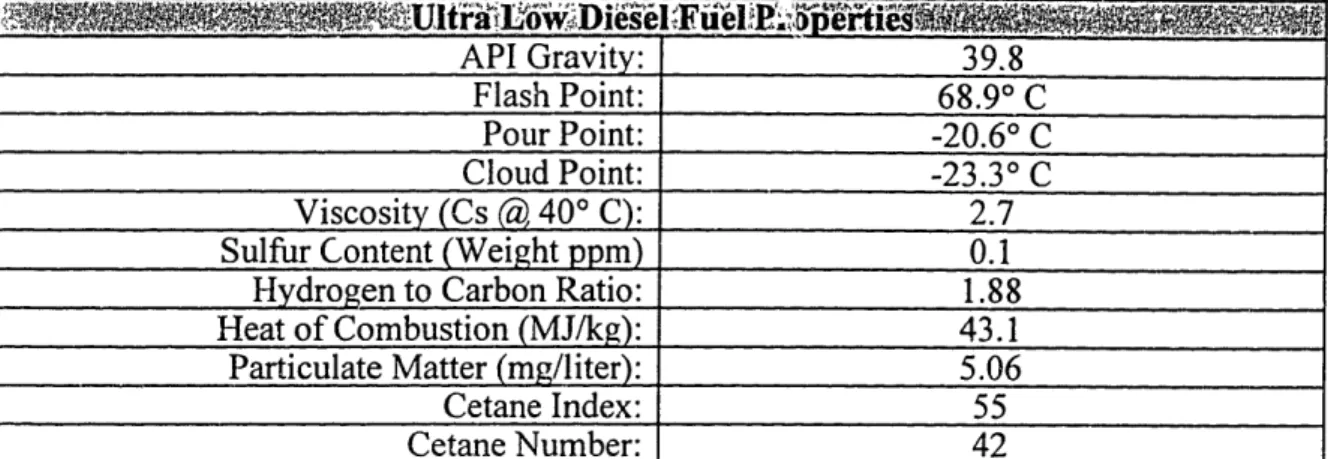
Lubrizol 30W oil was used in the engine during testing. Lubrizol 30W provided two advantages for the SO2 RTOC system. The first is that Lubrizol possesses a consistent sulfur content throughout the distillation fractions with good material balance (sulfur recovery). This eliminates the potential for false measurement of the oil consumption by ensuring that sulfur components do not vaporize and detach from the oil even though the oil is not consumed [10]. Secondly, since it was important to maximize (in comparison with other sources) the sulfur content in the engine oil, Lubrizol 30W with sulfur content - 1.27% sulfur by weight was ideal when used in conjunction with the ultra low sulfur fuel. The engine was run for 50 hours prior to conducting any testing to allow sufficient break in time for the oil. Table 3.2 and 3.3 provide lists of the fuel and oil properties.

MOPUlt

rao~DieserlrluelP:.:eit

-,

~.

I

i

'

Sulfur Content (Weight ppm) 0.1

Hydrogen to Carbon Ratio: 1.88

Heat of Combustion (MJ/kg): 43.1

Particulate Matter (mg/liter): 5.06

Cetane Index: 55

Cetane Number: 42

Table 3.2

Diesel Fuel Properties

Brand Lubrizol High Sulfur

Type SAE 30W

Sulfur Content (% by weight) 1.27

Table 3.3

Lubrizol 30W Properties

3.2.2 Sampling Procedures.

The SO2 analyzer was calibrated each day prior to testing. Detailed calibration and operating procedures can be found in Assessment of a Sulfur Dioxide Based System in Characterizing Real Time Oil Consumption in a Diesel Engine, by Jackson, May, 1996 [3]. The engine was run at 3200 RPM at high load (15 N-m) for approximately 45 minutes so that conditions would stabilize. Typically, once the SO2 system was calibrated, the engine conditions were stable and data collection commenced. Immediately after opening the engine sample pneumatic valve, bypass flow was adjusted to at least 1.5 liter/min. This was accomplished by throttling the flow of the engine exhaust, thereby producing sufficient back pressure to force the required bypass flow through the SO2 system. Exhaust manifold pressures were monitored to ensure that the engine operating conditions were not affected by the exhaust back pressure. Changes in exhaust back pressures were found to be insignificant for all operating conditions. OC I

data was collected for 40 minutes, the duration of one test sequence. Upon changing test conditions, the engine parameters (primarily oil out and exhaust temperatures) were again allowed to stabilize prior to resuming OC measurements.

3.3 Particulate Sampling System.

3.3.1 Particulate Sampling Theory.

Diesel particulate matter is composed of a carbonaceous core whose building blocks are carbon particles formed in the cylinder during combustion. These particles adhere to one another forming agglomerates that form the core of the diesel particulate of solids (SOL) [1, 14]. Once exhausted to the atmosphere, the exhaust gas is cooled and diluted by ambient air which initiates the adsorption and condensation process. At this point, some of the many products of incomplete combustion of the diesel fuel and engine oil absorb onto the carbonaceous material of the particulate. Figure 3.2, a reproduction from reference [1], displays the particulate formation process.

Time

Hydrocarbons

Cylinder

Dilution Tunnel

Figure 3.2

Particulate Formation Process

Nucleation Surface Growth I Agglomeration Adsorption and Condensation _ - - I --i I !

The objective of most particulate measurement techniques is to determine the amount of particulate being emitted to the atmosphere [1]. The intent of the dilution tunnel sampling system is to simulate release of the exhaust gases to the atmosphere. The exhaust is cooled by ambient air to a temperature of 52 C or less [1], initiating adsorption and condensation, and completing the particulate formation process. Particulate samples are then be collected by filtering the dilute exhaust gases. The specific procedure is described in section 3.3.2.

3.3.2 System Description.

A Mini Dilution Tunnel was constructed by Laurence [2] and used to collect particulate samples. This system was a scaled down version of an EPA Constant Volume Sample Dilution Tunnel similar to the one described by Wong [31]. However, the dilution tunnel was modified to dilute the entire exhaust flow vice only a fraction.

Particulate samples are collected simultaneously with oil consumption data during steady state operation of the engine at various speeds, loads, air intake pressures and with various piston ring configurations. The exhaust is directed through flexible stainless steel tubing into the main stream of the dilution tunnel. Previously, Laurence [2] and Ford [5] had used the dilution air as a means of creating suction, through a venturi, to draw the sample into the dilution tunnel, and as a temperature stabilizer. However, due to the need for a specified flow through the RTOC system, all the exhaust is directed into the dilution tunnel in order to provide sufficient back pressure and generate sufficient flow through the SO2 RTOC system. Therefore, the dilution air serves primarily as a temperature stabilizer for the exhaust stream. The dilution air, provided by shop air compressors, is filtered with a 2 inch Balston A15/80-DX filter to remove oil and moisture from the air (the stated removal effectiveness of the filter is 93% [2]). Concentrations of carbon dioxide are measured in both the raw and diluted exhaust lines to determine the dilution ratio. A sample of the exhaust mixture is then drawn through a 3/8" 316 stainless steel line, through a Pallflex Teflon coated 47mm glass fiber filter, P/N TX40HI20WW, mounted in a Graseby Anderson 316 stainless steel filter holder, P/N SE273. For better particulate adhesion, the Pallflex filters are installed in the holder with the teflon side of

the filter exposed to the sample flow. A Precision Scientific Petroleum Instruments Company Wet Test Meter is used in line, after the particulate filter, to measure the volumetric flow of the sample. A positive displacement vacuum pump is used to draw the sample through the collection system.

3.3.3 Sampling Procedures.

Initially, system calibrations were completed. The Wet Test Gas Meter was calibrated in accordance with ASTM D-1071 "Standard Test Methods for Volumetric Measurement of Gaseous Fuel Samples" [32]. A siphon was used to draw air through the meter which displaced a measured amount of water. The amount of water displaced is equivalent to the amount of air (gas) drawn through the meter. Several data points were collected and a calibration curve was developed, applied to the particulate sample volume data and is included in Appendix III. Additionally, the wet test gas meter was fitted with a telemetry system. This system was used to count the number of revolutions of the large pointer on the meter which was converted into the sample volume. As soon as the OC system was on line and sampling, a filter was loaded into the holder and wrench tightened to avoid o-ring bleed. The initial position of the large pointer of the wet test gas meter and sample start times were recorded. Sample collection was initiated by energizing the vacuum pump and opening the sample line isolation valve. Depending on the testing condition, the sample times ranged from 5 to 20 minutes. Adjusting the dilution ratio lengthened and/or shortened the required sample time. CO2 concentrations were

measured every three minutes for the duration of the test period. Halfway through the period, the CO₂sample was switched from raw to dilute via the three way valve shown in Figure 3.2 to obtain the dilution ratio. Once the system (between the sample isolation valve and the wet test gas meter) had stabilized, system temperatures were recorded. Close attention was paid to the line temperatures before and after the filter to ensure temperatures were below 52 C [1] throughout the duration of sample collection. Maintaining the filter face temperature below 52 C helped to ensure the proper adsorption and condensation of hydrocarbon on the carbonaceous fraction of the particulate [14]. Additionally, it was attempted to maintain the filter face temperatures

constant at +/- 2 C between repeated test conditions. This has been reported to aid in obtaining consistent particulate data. It has been shown that dilution tunnel temperature has a greater effect on the process of adsorbing hydrocarbons onto solids (producing SOF) than does the actual hydrocarbon concentration in die tunnel. More consistent data was obtained when the filter face temperatures were held constant [14]. However, for this system, adjusting the dilution tunnel temperature during particulate collection would have altered the sampling conditions thereby providing erroneous results. Therefore, dilution tunnel and engine operating conditions were closely monitored and reproduced to obtain the constant filter face temperature between repeated test runs. The results showed that approximately 60% of the test conditions maintained filter face temperatures within +/- 2° C, while the remaining 40% were within 6°C.

At the completion of the sampling period, the final position of the large pointer of the wet test gas meter and the total number of meter revolutions were recorded and the filter was placed back into its casing, taped closed, doubled sealed in ziploc bags, and placed in storage at a temperature of less than 4° C. At this point a second filter was placed in the holder and the procedure was repeated. Two particulate samples were collected per test run for each test condition for ring pack one. One particulate sample was collected per test run for each test condition for ring packs two and three. The typical time sequence of events is outlined in Table 3.4.

ifitioy nuraio

Minute 0 Commenced Emissions Measurement. 40 min (3 min intervals)

Minute 1 Set up for Particulate Sampling. 1 min

Minute 2 Commenced Particulate Sampling #1. 15 min

Minute 15 Recorded all Pertinent Data. 1 min

Minute 17 Secured Particulate Sampling #1. 2 min

Minute 18 Switched to Dilute Emission Measurement 1 min

Minute 20 Commenced Particulate Sampling #2. 15 min

Minute 35 Secured Particulate Sampling #2. 5 min

Minute 40 Secured from Test Sequence

Table 3.4

A diagram of the dilution tunnel is shown in Figure 3.3. Particulate C::l&-- llees. . h h Figure 3.3

Particulate Sampling System

3.3.4 Sample Analysis.

Batches of 25 filters were sent to ORTECH Corporation for analysis. ORTECH Corporation was contracted to determine filter loading, soluble organic fraction (SOF), fuel / lube oil contributions to the SOF and to conduct Gas Chromatographic / Mass Spectrometry (GC/MS) analysis on specified samples. Upon receipt, ORTECH placed all the samples in a climate controlled conditioning room to equibrilate overnight. Samples were then examined, weighed to determine filter loading and prepared for extraction. Extraction was completed with 100% Methylene Chloride which partitioned the sample into a soluble fraction and a dry insoluble fraction. Each sample was again conditioned and the extracted weight was determined in order to tabulate the soluble organic fraction (SOF) and the insoluble fraction (Non-SOF).

A quantitative analysis of specified samples was then conducted to determine what percentage of the SOF was derived from the lubricating oil that had been consumed.

The fractions of fuel and lubricant in the particulate samples were determined using a ratio of integrated times obtained from chromatograms of three samples; 1) the extracted SOF, 2) the "topped" fuel, and 3) the new !ube oil. (The "topped" fuel is the remainder of the fuel after 30% by volume is distilled.) [18] The precision of the lubricant derived portion of the SOF results is on the order of 0.001 g/bhp-hr.

3.4 Test Matrix Development.

The test matrices were developed based on a duty cycle that models near land and maneuvering type operating conditions. In order to determine what a "complete" marine duty cycle would be, ISO 8178 Part 4, "Reciprocating Internal Combustion Engines-Exhaust Emission Measurement" [24] was evaluated. Although these cycles do not effectively describe the duty cycles of Coast Guard and Naval vessels, ISO 8178-4 is the only current standard available for commercial ships. The test cycles for different engine applications as outlined in ISO 8178-4 are shown in Table 3.5. The cycle definitions are listed in Table 3.6.

A Reference cycle for vehicle engines

B Universal cycle, applications similar to on-road service

C1 Off-road vehicles and industrial equipment, med and high load C2 Off-road vehicles and industrial equipment, low load

D1 Constant speed applications, power plants

D2 Constant speed applications, generator sets with intermittent load El Marine engine applications, pleasure craft engines

E2 Marine engine applications, constant speed engines for ship E3 Marine engine applications, heavy-duty propulsion engines

F Locomotive applications

G1/G2 Small engines, utility lawn and garden G3 Small engines, hand held equipment

Table 3.5

The duty cycles considered to be applicable for simulation of low speed marine diesel engine operations were cycle E2 (Marine applications, constant speed engines for ship propulsion) and cycle E3 (Marine applications, heavy duty propulsion engines). Cycle E2 applies to constant speed diesel engines and is not applicable to this study. The unmodified version of the E3 duty cycle would require four engine testing speeds and loads as shown in Table 3.6. However, time constraints demand that the scope of this study be limited to ensure ample time for data analysis. Therefore, a modified version of the E3 duty cycle was selected to model operating conditions for low speed marine diesel engines.

The lowest recommended test speed for the E3 duty cycle, 63% of maximum, does not adequately model near land or maneuvering operating conditions. For this reason, an "idle" speed was added at 35% of maximum rated speed (1200 RPM). The Ricardo Hydra engine is a small bore, high speed diesel engine and the intent of this study was to model low speed marine diesel engines. For this reason, high end test speeds of 70% and 97% (2400 and 3200 RPM) vice 80%, 91% and 100% of maximum rated speed were incorporated. These chosen values matched the work completed by

Schofield [4] and Ford [5], which was ideal for evaluating repeatability of test results, and they sufficiently cover the suggested E3 duty cycle test speeds. The modified E3 duty cycle utilized in this study included three test loads vice two. A mid-range test load was added to provide a more complete range of loading conditions. This approach met the requirements for this study and sufficiently incorporated the guidance of ISO 8178 Part 4.

>2v0.

rI,

eD

3t>1ST8178V4

iffe r

Idle 60 Percent of Rated Speed Rated Speed

Cycle _{_ ~:¥ :? ,}: ~ _, " ' _{i . , ,:: "'} Percent Load _{e c n ,a ~~':: ~/ '"?~? '} i ~ ~:_{... ''}

Table 3.6

ISO 8178-4 Engine Cycles

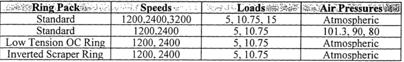
Table 3.7 outlines the specific testing conditions contained in the modified E3 duty cycle. The four resultant test matrices and labeling system are further described in the following sections.

*Wows

tRinga .

s Speeds-,

Lob

.

;Air

Pressures

Standard 1200,2400,3200 5, 10.75, 15 Atmospheric

Standard 1200.2400 5, 10.75 101.3, 90, 80

Low Tension OC Ring 1200, 2400 5, 10.75 Atmospheric

Inverted Scraper Ring 1200, 2400 5, 10.75 Atmospheric

Table 3.7

Modified E3 Duty Cycle

3.4.1 Test Matrix Labeling.

In order to effectively track each test condition, a labeling system was developed. This allowed for easy recognition of test conditions, and ensured that all conditions were covered prior to and during testing. To this end, the following system of letters and numbers worked very effectively. It is important that this system be described to ensure a

clear understanding of the test matrices. There were three primary types of test conditions; 1) Standard runs, 2) Load transients, and 3) Speed transients. The standard runs consisted of a specific speed, load and intake manifold air pressure. No particulate data was collected during the transient conditions. Details of those matrices can be found in Jackson [3]. Figure 3.4 describes the labeling system for each test matrix used in this study.

Standard Runs.

I - A - I - A - 1

Number Letter Number Letter Number

Ring Speed Load Air Run

Pack Pressure

Definition of Numbering and Lettering System.

Ring Pack: 1 = Standard Ring Pack 2 = Low Tension OC Ring 3 = Inverted Scraper Ring Speed: A = 1200 RPM

B = 2400 RPM C = 3200 RPM Load: I = Low Load (5 N-m)

2 = Medium Load (10.75 N-m) 3 = High Load (15.1 N-m)

Air Pressures: A = Standard Air Pressure - 101.3 kPa B = 90 kPa

C = 80 kPa Run Number: I = Run One

2 = Run Two 3 = Run Three 4 = Run Four

Figure 3.4

Test Matrix Labeling System

3.4.2 Test Matrices Descriptions. Standard Ring Pack Test Matrix.

The standard ring pack test conditions were varied for three speeds and loads in an attempt to model near land / in port operating conditions of a marine diesel. Initial intentions were to obtain data for each condition of the three by three matrix, but as

testing progressed it became evident that the high load condition for low and medium speeds provided very erratic oil consumption data. The RTOC system quickly became saturated with heavy particulate deposits which resulted in several hours of run time to purge and return to normal sampling conditions. Time being a factor throughout testing, it was decided that the remaining high load operating conditions would be dropped for the low and medium speeds. At least one data point was collected for each high load condition. All other data points in the matrix were run four times for repeatability. The standard ring pack test matrix is shown as Table 3.8.

= Selected for Fuel/Lube Contribution Testing = Selected for G/MS Tstin

Speed Speed Speed

1200 Fil# Fil # MS 2400 Fil# Fil# MS 3200 Fil # Fil# MS

___ A 127 ^k XW JBIAI 17 8 11

Low IAIA2 39 40 25 25 VBA22 1 13 4

IA 1 A3 41 42 __ '_ M3MA ;,1M 52 I C 1 A3 7 38

1I A 4 69 70,X1 IB1 A4 53 54 C1 A4 63 62 IA2A1 9 10 X 1B2AI 5- 6 1C.2A 1 3 4

Med J12A;S1 24' 48 1 B2MA2 19 120% 'X 15 r6&.,!

1A2A3 49 50 ,lB2A,3 29 'go2A3O :1/0 18

1A2A4 67 68 1IB2A4 65 66 1C2A4 61 62

IA3A 1 35 36 61 B 31 3A1 21 22

High IA3A2 Deleted I'B3.A2. 34 _ 1C3A2 23 24

1A3A3 Deleted 1B3A3 Deleted 58

1A3A4 Deleted 1B3A4 Deleted :1G3~ 59i 60 X

Table 3.8

Standard Ring Pack Test Matrix

The ring pack configuration was the standard as set by the manufacturer's specifications. The first ring, or compression ring, was chrome plated and slightly rounded in shape. The second ring, or scraper ring, was beveled. The third ring, or oil control ring was chrome plated with two rails and a separate coil spring for tension control. Table 3.9 shows the manufacturer's specifications.

R~in ~ i< WDiamedtenmmi Cld a mmi

Compression 80.25 0.43 9.3

Scraper 80.25 0.43 8.2

Oil Control 80.25 0.51 53.8

Table 3.9

Standard Ring Pack Characteristics

Standard Ring Pack; Varied Air Intake Pressure Test Matrix.

The engine was run at low speed (1200 RPM) and at low load (5 N-mr) while the air intake manifold pressure was varied over three pressures; 1) 101.3 kPa, 2) 90 kPa and 3) 80 kPa. 1200 RPM was selected as the operating condition to vary air pressure since it had been shown that the particulate rate was greatest at low speed [5]. Time and quality of data being major factors, only the low load condition was tested as it provided very consistent oil consumption results compared with the medium load condition as shown in Figures 3.5 and 3.6. The ring pack characteristics are shown in Table 3.9. Each test was run four times for repeatability. The standard ring pack-varied air intake pressure test matrix is shown as Table 3.10.

1.-~ i= elected for GCIMS Testing

Speed 101.3 kPa Speed 90 kPa Seed 80 Pa

1200 Fi # Fil # MS 1200 Fil # Fil # MS 1200 Fil # Fi # MS

i191 27 1AIBI 43 44 _92=217 76

Low 1AIA2 39 40 1AI1B2 4 6 1AC2 77 78

IAIA3 41 42 K11ThIB3 7 1 A13 71 9 80

__

AN4!

69 WN

X

lai

73

l

2

Table 3.10

Standard Ring Pack, Varied Air Intake Pressure Test Matrix RA O WI = Selected for Fuel/Lube Contribution Testin ...

Oil Consumption Data for 1200 RPM - Low Load

__

Figure 3.5

Oil Consumption

@

Figure 3.6

Oil Consumption @ 1200 RPM - Medium Load

9 20 a 15 .o 0 E 0 5 O 0 O O O O O o O o o O o O o O O O o O O 0O cn ( 0CD ) N Uz W o - T (c C o N N u) - -" N N CS (f) M M (M V V U) LO L U) Time (sec)

Oil Consumption @ 1200 RPM - Medium Load

9 R 0.v a, 0 0. 0 5. 00 _{) (} 0 0 00 _{) N ND N- 0} 0 ₀ 0 0 00 0 _{r- 0 cO} 0 0 0 0 0 0 0 0_{c O 0 N to CO c o - ,,} rN N im (c) M s M e) M V U) U0 U) Time (sec) . _ _._ _ _ : , I , : : , i , ! i , i i i . , , i i i i i , ! I i i i , i i i i i i : : : : , ; , : : : 1 : : : : : 4 : 1 : : : : i : : : : :

Ring Pack Number Two Test Matrix (Low Tension OC Ring).

Testing was completed for two speeds and loads for the second ring pack configuration.. As was the case for the standard test matrix, the high speed and high load conditions were dropped for this testing matrix. The increase in oil consumption for each condition (not just high speed and load) was significant, and was initially off-scale with this system. Dilution of the exhaust sample with zero air (sulfur dioxide content < 0.5 ppm) brought the low / medium speed and load conditions back onto scale, while high speed and load remained off-scale. The ring pack specifications are shown in Table 3.11. All tests were run four times for repeatability. The ring pack number two test matrix is shown as Table 3.12.

Rn>

Di

ii

t&

. t

... W.

d

im'

siC

ok

Compression 80.25 0.43 9.3

Scraper 80.25 0.43 8.2

Oil Control 80.25 0.51 28.01

Table 3.11

Ring Pack Two Characteristics

= Selected for Fuel/Lube Contribution Testin Selected for GC/MS Tsting

_S Sveed SpeedSpeed

1200 Fil Fil # MS 2400 Fi# Fil M 3200 Fil# Fil # MS

2A1AI 83 2B1AI 91

Low SX 2B 1 A2 92 .

2A 1 A3 85 Btf3 9

2AI4 86 2BA4 2BA 4 94

2A2A1 87 2B2A1 95

Med 2A2A2 88 - 12 2,9 !5__ Not Tested

. 0-9' 2B2A3 97 Time Limitations

2A2A4 90 2B2A4 98 _

2A3A1 Deleted 2B3A1 Deleted __

High 2A3A2 Deleted 2B3A2 Deleted 2A3A3 Deleted 2B3A3 Deleted 2A3A4 Deleted 2B3A4 Deleted

Table 3.12

Ring Pack Number Three Test Matrix (Inverted Scraper Ring).

Testing was again completed over two speeds and loads for the third ring pack. The high speed and load conditions were dropped for the reasons outlined above for ring pack 2. Tests were run two times for repeatability as the time schedule did not allow for additional testing. The ring pack specifics are as shown in Table 3.9 with the scraper ring inverted. The ring pack number three test matrix is shown as Table 3.13.

= Selected for GC/MS Testing

Seed 101.3 k kPa Seed 8090 kPa

1200 Fil # Fil # MS 2400 Fil # Fil I MS 3200 Fil# Fil# MS

Low /g St. AF t,:Iq, CR ,990BEA-14

3 A1A2 106 3B1A2 100 Not Tested

Med J.03- A IS9 3B2A1 IIKS 101 Time Limitations

3A2A2 104 1kt.I IXfl32AL: OMN

Table 3.13

Ring Pack 3 Test Matrix

It should be noted that test runs for matrices two and three were consistently run back to back versus randomly. This had to be done in order to obtain a value for the

dilution ratio of the exhaust sample and injected zero air. Without this information, the OC results were unobtainable. The details of this procedure can be found in Jackson [3].

Gas Chromatographic / Mass Spectrometry Sample Matrix.

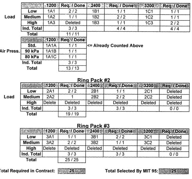
Particulate samples were selected for GC/MS testing in accordance with the Statement of Work for ORTECH Contract El 11B004895. The primary requirement of the contract was to conduct GC/MS analyses on 25 samples for the purpose of identifying specific compounds found in the SOF, and approximating their relative amounts. One of each set of 4 test runs from the standard test matrix was selected for analyses (9 total). A second sample was analyzed for 1) low speed-low load, 2) medium speed-medium load, and 3) high speed- high load for each ring pack (7 total) . A third set of samples was analyzed for the standard ring pack with varied air intake manifold pressures. One

sample from each condition (3 total). The remaining six samples were designated by this study. The matrix used for tracking the GC/MS samples is shown below in Table 3.14.

Ring Pack # 1

Load

Air Press.

Load

'~,~-,

200,

.ReI Done..

CRe

. Req,

.Done

,

0

"2

;Dh

Low 1A1 2/2 1B1 1/1 1ci 1/1

Medium 1A2 1 /1 182 2 /2 1C2 1 /1

High 1A3 Deleted 1B3 1 /1 1C3 2/ 2

Ind. Total 3/3 4/4 4/4

Total 11 /11 .... 1200 'Req/.DoneI

Std. 1A1A 1 / 1 <= Already Counted Above

90 kPa 1A1B 1 /1 80 kPa IA1C 1 / 1

Ind. Total 3/3

Total 13 /13

Rina Pack #2

'Y .200 'Req'. Don ., r.... : Don ,3200 Req. iDo, e

Low 2A1 2 / 2 2B 1 / 1 2C1 Deleted

Medium 2A2 1 2B2 2 /2 2C2 Deleted

High Delete Deleted Deleted Deleted Deleted Deleted

Ind. Total 3/3 3/3 0/0 Total 19 /19 Low 3A1200 Low 3A1 Medium 3A2 High Delete Ind. Total _ Total KIln , Re. cq!iDdone' 1/1

2/2

3/3

Deleted Deleted Deleted Deleted

3/3

0/0

Total Required in Contract: Total Selected By MIT 95:

Table 3.14 GC/MS Sample Matrix

3.5 ENERAC 2000ET' and MIT Gas Cart Set Up.

3.5.1 ENERAC 2000ETM_.

The ENERAC was set up to take samples from the exhaust mixing tank located in line with the engine exhaust. This location was selected for two reasons; 1) to simulate an engine exhaust stack found in shipboard applications; and 2) to ensure sufficient exhaust temperatures at the sample port to avoid condensation of the exhaust gases. To avoid damaging the probe, close attention was paid to the temperature surrounding the probe housing to ensure that it did not exceed 71° C, and to the temperature inside the mixing tank to ensure that the sintered filter was not exposed to temperatures in excess of 1038° C [23]. These temperatures were the maximums designated by instruction manual [23]. The sample was drawn through the probe housing which contains a permeation drier, whose function is to remove the excess water vapor that is present in the sample. Since NO2 dissolves readily in water, any condensation present in the hose assembly would result in erroneous readings [23]. A section of clear tubing is located immediately following the probe assembly for monitoring any condensation buildup in the hose assembly. The sample was drawn through the system via a double bellows pump located in the ENERAC briefcase. Gas passes through a Carbon Monoxide (CO) electrochemical sensor and then through an Oxygen (02) electrochemical sensor. The sample then enters a cavity inside the housing where the Nitric Oxide (NO) and Nitrogen Dioxide (NO2)

electrochemical sensors are exposed. NOx concentrations were calculated by the ENERAC by simply adding the concentrations of NO and NO₂. A diagram of the ENERAC set up is shown below in Figure 3.7.

The ENERAC was calibrated in accordance with the instruction manual procedures [23] prior to conducting testing. The following gases were used for the calibration; 1) 948 ppm NO, 979 ppm CO with less than 2 ppm NO2; and 2) 573 ppm NO2 with less than 1 ppm NO. The oxygen sensor was calibrated with ambient air, and with calibration gases containing 02 concentrations of 1.97% and 8.25%. The

concentration of CO2 is calculated by the ENERAC and it is only a function of the oxygen concentration and the type of fuel used in the engine. Therefore, the only

calibration requirement was the proper selection of fuel type. Selecting the proper fuel type is critical to the computation of CO2. The ENERAC has several factory set fuel types that list the respective heats of combustion. Fuel 1 had a heat of combustion of 43.3 MJ/kg and it was selected since the ultra low sulfur diesel fuel had a heat of combustion of 43.1 MJ/kg. The significance of this difference is addressed in Chapter 5. Midway through testing, calibration was checked and found to be within 10% of the calibration gas concentrations, which was consistent to the initial calibration values. Calibration curves were constructed for each ENERAC sensor, applied to the emission results and are included in Appendix III.

At the start of each day of testing, the ENERAC was auto-zeroed, allowed to properly warm up and stabilize prior to sampling. Gaseous emission data were collected simultaneously from the ENERAC and the MIT Gas Cart during steady state and transient operating conditions throughout the completion of the standard ring pack and standard ring pack with varied air intake pressure test matrices. CO, CO2, 02, NO and NOx were the five gases measured for this comparison. A statistical analysis was completed to determine the relativistic trends between the two gaseous emissions detector systems and can be found in Chapter 5. A description of the MIT Gas Cart set up is found in section 3.5.2.

ch

Figure 3.7

ENERAC 2000ETM _{Set Up}

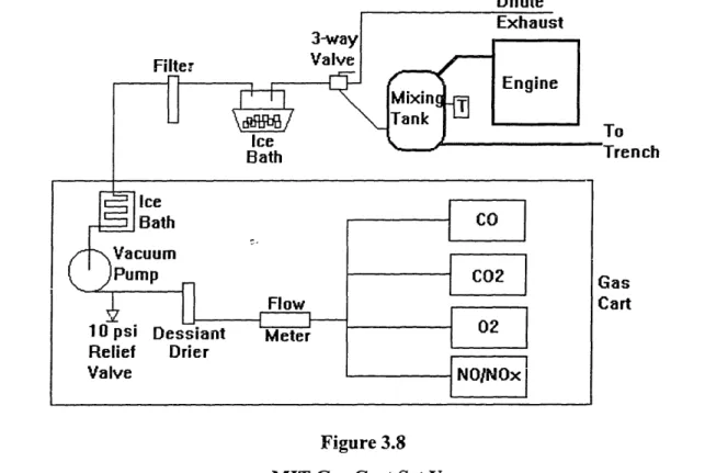
3.5.2 MIT Gas Cart Set Up.

The MIT Gas Cart utilizes a combination of infrared, polarographic and chemiluminescent sensors to detect CO (infrared radiation technique), CO2 (infrared radiation technique), 02 (polarographic partial pressure technique), NO (chemiluminescence) and NOx (chemiluminescence) in engine exhaust. The analyzers are rack mounted in a large semi-mobile cart. Exhaust samples were taken from the mixing tank in the same vicinity as the ENERAC connection. The heated line configuration used previously by Laurence [2] was removed as it was considered more of a fire hazard than a necessary requirement for exhaust sampling. A positive displacement vacuum pump draws the sample through a 3-way valve, used to control the selection of raw or dilute exhaust samples, and through an additional ice bath. This additional ice bath (external to the gas cart) Awas added to remove water vapor from the sample to avoid damaging the

vacuum pump. An additional filter was also added (external to the gas cart) prior to the vacuum pump to remove excessive particulate matter in the exhaust. Major vacuum pump overhaul was required midway through testing due to the extensive buildup of particulate matter at the intake and exit ports of the pump. The, addition of these two items allowed the system to operate without further problem. From the vacuum pump, the sample was directed through another ice bath and desiccant drier for conditioning, a flow meter and into each respective analyzer. The output read from the CO and CO2 analog meters was converted into concentrations via the corresponding Table 2 in the gas cart handbook [25]. Concentrations for 02, NO and NOx were read directly from the analyzer. A diagram of the gas cart set up is shown in Figure 3.8.

Dilute

0

rench

art

Figure 3.8 MIT Gas Cart Set Up

The gas cart was calibrated at the start of each day of testing. All sensors were initially purged with nitrogen to clean out any remaining exhaust sample and ambient air conditions. Sensors were then tuned, zeroed, and calibrated. Three calibration gases

were used for this process; 1) 8.08% CO2, 4.87% CO and 1.97% 02; 2) 3.07% CO2, 1.05% CO and 8.25% 02; and 3) 2692 ppm NO. The NOx sensor was calibrated with the same gas as the NO sensor as the NO2 concentration was less than 2 ppm. Calibration curves were constructed for each sensor, applied to the emission results and are included in Appendix III. Detailed instructions for the operation and calibration of the gas cart are found in "The MIT Gas Cart Operation Handbook", by Miller, May 1996 [25].