Adaptive Load Control of Microgrids
with Non-dispatchable Generation
by
Kevin Martin Brokish
B.S., University of Colorado (2007)
MASSACHUSETTS INSTfT E OF TECHNOLOGYAUG 0 7 2009
LIBRARIES
Submitted to the
Department of Electrical Engineering and Computer Science
in partial fulfillment of the requirements for the degree of
Master of Science in Electrical Engineering
at the
MASSACHUSETTS INSTITUTE OF TECHNOLOGY
June 2009
@ Massachusetts Institute of Technology 2009. All rights reserved.
A uthor ...
---..
..
..
..
. ..
..
..
..
.
Department of Electrical Engineering and Computer Science
May 8, 2009
Certified by....
Dr. James L. Kirtley, Jr.
Professor
Thesis Supervisor
/)
Accepted by.
/
Dr. Terry P. Orlando
Chairman, Department Committee on Graduate Theses
ARCHIVES
Adaptive Load Control of Microgrids
with Non-dispatchable Generation
by
Kevin Martin Brokish
Submitted to the Department of Electrical Engineering and Computer Science on May 8, 2009, in partial fulfillment of the
requirements for the degree of Master of Science in Electrical Engineering
Abstract
Intelligent appliances have a great potential to provide energy storage and load shed-ding for power grids. Microgrids are simulated with high levels of wind energy pene-tration. Frequency-adaptive intelligent appliances are deployed and optimized within the simulation, indicating the usefulness and feasibility of these loads on microgrids. The economic feasibility and implementation of these appliances is also discussed.
Thesis Supervisor: Dr. James L. Kirtley, Jr. Title: Professor
Acknowledgements
I would like to thank Dr. Jim Kirtley for his insight and guidance on this project. Once I had determined Markov Chains were incapable of modeling what I hoped they could, it was Dr. Scott Kennedy's idea that I write about it. The math in Chapter 2 came from brainstorming sessions with Ozan Candogan. Thanks to Dr.
Hatem Zeineldin and Dr. Mirjana Marden for their insights on microgrids. Finally, I am deeply grateful to the MIT-Portugal program for its sponsorship of this work.
Contents
1 Introduction
1.1 Description of FAPERs ...
1.2 Thesis Layout . . . .
2 Wind Power Modeling
2.1 Introduction...
2.2 How Markov Chains Work ...
2.2.1 Mathematical Description ...
2.2.2 Higher Order Markov Chains . . .
2.3 Using Markov Chains to Model Wind . . . 2.3.1 Markov Chain Creation ...
2.3.2 Wind Speed or Wind Power? . . .
2.3.3 Appeal of Markovian Wind ....
2.4 R esults . . . .
2.4.1 Autocorrelation ...
2.4.2 Autocorrelation Error ...
2.5 Why Markov Wind Models Are Dangerous
2.5.1 Underestimated Storage . . . . 21 . . . . 2 1 . . . . 2 1 . . . . . 2 2 . . . . . 23 . . . . . 23 . . . . 24 . . . . . 2 5 . . . . 26 . . . . 28 . . . . 29 . . . . 3 1 . . . . . 33 . . . . . 3 3 2.5.2 Not Accurate for FAPER Simulations . ... 33
3 Microgrid Model and Simulation 35
3.1 W hat is a M icrogrid? ... ... . 35 3.2 Simulated M icrogrid ... 37
3.2.1 Simulation Description ... .... .. . . ... . . 38
4 FAPER Model 41 4.1 Linear Approximation of Appliance Behavior .. ... 41
4.2 FAPER-capable Appliances . ... . . . ... . . . . 43
4.2.1 Refrigerators and Freezers ... ... . 43
4.2.2 Air Conditioners and Electric Heaters . . . ... . . 44
4.2.3 Hot Water Heaters, Clothes Driers, and Dish Washers . . . . . 44
4.2.4 Pool Heaters ... ... . . . 45
4.2.5 Shorten Time to Hibernate . ... . 45
4.2.6 Plug-in Hybrid Electric Vehicles ... . 45
4.3 FAPER Simulation Setup ... .. . . . . . 46
5 Insights to Optimal FAPER Control 49 5.1 Literature Survey ... ... .. ... ... ... . 49
5.2 Observations and Insights into FAPER Control . . .. . . . ... 51
5.3 Probabilistic Algorithm ... ... ... . .... ... 53
5.3.1 Optimization of Control Algorithm . . . ... ... . 55
5.3.2 Results and Comparison ... ... . . . . . . 57
6 Analysis of FAPER Behavior 59 6.1 Semi-Linearity ... .... . ... 59
6.1.1 Definition of Variables ... ... . . . .. . . . 59
6.1.2 Linear for Slow Frequency Changes ... .. . . .. .. .. 60
6.1.3 Nonlinear for Rapid Frequency Changes . . . . ... . 61
7 Viability and Implementation 63 7.1 Economic Viability ... ... ... . . . . . . . . 63
7.2 Implementation Via Retrofitting ... .. . . . . 64
7.3 Future Research ... ... ... . ... 66
7.4 Conclusion ... ... 67
A Wind Power Modelling 69
A .1 M atlab Code . . . 69
A.1.1 Profile Creation ... 69
A .2 Prim ary Script .. .. ... ... .. .. ... . . . .. .. .. 71
A.3 Markov Chain Generator ... 72
A.4 Monte Carlo Data Generator ... 73
B FAPER Simulation 75 B.1 M atlab Code . . . .. . . . 75 B .1.1 M ain . . . . 75 B .1.2 Setup . . . 77 B.2 Simulink Blocks ... 78 B.2.1 Appliance Block ... 78
B.2.2 Other Simulink Blocks ... 81
List of Figures
1-1 Sample FAPER Control Algorithm ...
2-1 A simple first-order Markov chain for wind power modeling . 2-2 Markov Chain Disparities ...
2-3 Autocorrelation Plot 1 . ...
2-4 Autocorrelation Plot 2 . ...
2-5 First Order Autocorrelation Error . ...
2-6 Second Order Autocorrelation Error . ...
2-7 Third Order Autocorrelation Error . . . .
2-8 Storage Estimates and RMS Error . ...
3-1 A Simple Microgrid ...
3-2 Simplified Simulation Block Diagram . . . . 3-3 Full Simulation Block Diagram . . . .
4-1 Household Electricity Consumption Makeup ...
5-1 Control Function from Homeostatic Utility Control 5-2 Control Function from Stabilization of Grid Frequency
namic Demand Control . ...
5-3 FAPER Instabilities ... 5-4 FAPER Clusters ...
5-5 New FAPER Algorithm ... 5-6 Pareto Frontier . ...
5-7 FAPER Temperatures Over Time . ...
. . . . 38
. . . . . 39 . . . . . 40
Dy-5-8 Non-Probabilistic FAPER Temperatures . . . . 5-9 Pareto Frontier Algorithm Comparison . . . . 6-1 Variables Used in FAPER Analysis for Small mbound 6-2 Variables Used in FAPER Analysis for Large mbound
B-1
B-2 B-3 B-4
Power Calculation Simulink Block . . . .. Droop Generation Simulink Block . . . ... Gain Calculation Simulink Block . . . ... Grid Frequency Simulink Block . ...
. . . . . 58 . . . . . . . 58 . . . . . 60 . . . . . 6 2 .. . . . . 81 .. . . . . 81 .. . . . . 82 ... . . . . . 82
List of Tables
Chapter 1
Introduction
The era of cheap fossil fuel energy is drawing to a close: fuel prices are becoming
increasingly volatile as global demand increases, the science behind dire ecological impacts of continued carbon emissions is generally accepted, and national energy
security permeates political discussions. Society places great hopes on renewable energy sources such as wind and solar, but these are non-dispatchable: they produce
predictable but variable quantities of power.
On hourly and daily timescales, non-dispatchable power generation must be bal-anced by other forms of power generation or by energy storage. On windless days in
Denmark, for example, energy is imported from neighboring countries, and on windy days, excess energy is exported [36]. Norway, which has the most hydro-powered gen-eration per capita in the world [39], can effectively act as energy storage for Denmark: hydro power generation is relatively easy to start and stop to balance wind, and while
it is stopped, energy is stored as water fills reservoirs. Not all countries have such resources at the necessary scale (or neighbors with such resources), and the risk and integration problems that come with high penetration of renewables has stimulated a flurry of research in microgrids.
Microgrids are essentially islandable partitions of a large power grid paired with an added layer of intelligence. The two chief benefits of microgrids are the ability to effec-tively integrate micro distributed generation, and the ability to intentionally island. The first is achieved because the microgrid appears like a single producer/consumer to
the rest of the power grid. The Consortium for Electric Reliability Technology Solu-tions (CERTS) Microgrid Concept paper claims that "the CERTS MicroGrid concept eliminates dominant existing concerns and the consequent approaches for integrating [distributed energy resources]" [32]. This is partially true in that microgrids effectively delegate protection and coordination issues to the microgrid managers rather than the utilities, and may open the door for more home generation such as photovoltaic roofs. The second benefit of microgrids is the ability to disconnect and function as an island, weathering catastrophic failures on the larger grid. This increases user reliability because without islanding capability, consumers on the microgrid would be dragged into a brownout or blackout along with the rest of the grid.
Microgrids, however, do not specifically solve the problem of balancing load and generation. Energy storage and backup generation on large scales are still required in
order to balance non-dispatchable sources of energy. In fact, on islanded microgrids
(and small power grids in general), regulation is also a problem on shorter timescales. If a cloud were to pass over a photovoltaic array connected to the vast Eastern In-terconnect power grid, the drop in power would go virtually unnoticed. But on an islanded microgrid, where generation from a PV array makes up a significant portion
of the generation, a cloud passing overhead could cause a major problem. Other gen-eration or energy storage must be available to provide a fast influx of energy. Neither
backup generation nor energy storage are appealing because the cost of renewable energy is already greater than the cost of energy produced by fossil fuels, and backup generation and storage add to the net cost of deploying non-dispatchable power
gener-ation. This is the motivation for researching "Frequency Adaptive Power and Energy Reschedulers" (FAPERs) [34].
1.1
Description of FAPERs
First introduced nearly 30 years ago by MIT professor Fred C. Schweppe, the FAPER concept is to turn people's temperature-bounded appliances into energy storage using grid frequency as a signal. Many homes have on/off loads that cool or heat water or
air within a given temperature range. They repeatedly heat until the upper bound
is reached and cool until the lower bound is reached. Air conditioners, electric space heaters, and refrigerators are the most obvious appliances to become FAPERs, but
there are others as well. These units all go through cycles of heating and cooling. It does not particularly matter when they are on or off-users would not notice if their
well-insulated refrigerator stayed off for an extra few minutes. FAPER appliances
would turn on and off as a function of their current temperature and power grid frequency, as illustrated in Figure 1-1. If there is not enough power generation on a
synchronous machine-driven power grid, the frequency decreases below the standard frequency of 60Hz (50Hz in most parts of the world). Conversely, if there is too much
power generation, the frequency increases above the standard frequency. In this way, FAPERs act as load shedding: they turn off when there is a power shortage (low
frequency). They also act as energy storage because extra cooling or heating occurs during high frequency periods so the unit can essentially ride through low frequency periods on the heat/coolness that it already has. In addition to the aforementioned appliances, FAPER candidates include other loads like pool heaters and even some non-heating/cooling loads such as electric vehicles.
Temperature
rF
Ai
Frequency
Figure 1-1: Control algorithm for a FAPER-enabled cooling appliance
The frequency of grids as large as the Eastern Interconnect do not deviate much from the nominal value, but the frequency of small microgrids in islanded mode will fluctuate wildly in comparison and may be a challenge to control. The typical way to compensate for sudden variations in power generation and load is with spinning reserve: partially loaded or idle generators that regulate frequency and can instantly
1
supply emergency power. That is an expensive solution, and it is a pollution-intensive solution that would become even more expensive in a country with a carbon tax or emissions trading scheme. Some have suggested battery banks or flywheels as an environmentally friendly alternative to spinning reserve, but both of these options are more expensive than spinning reserve at present.
Replacing spinning reserve with FAPERs on large grids has been cursorily ex-plored [37]. Master-slave with frequency droop control is the typical control method-ology for the control of microgrids, but there are others as well [26]. Even inverters can be controlled in a way such that they behave with a synchronous machine-like droop characteristic [13]. In Chapter 6, it is proven that, given steady state opera-tion, FAPERs act similarly to a distributed droop control. However, the response of FAPERs when the group of them is not in steady state is complicated, and undesir-able behaviors can arise. For example, cold load pickup[3]-like behavior can occur. Mitigating undesirable behaviors is one of the principle areas of study for this thesis. Little attention has been paid in the literature to optimizing control strategies of FAPERs. References [37] and [7] utilize algorithms that are either potentially unstable or too slow to respond in an effective manner on a microgrid. An experiment was carried out in [27] where simple under-frequency load shedding FAPERs were actually deployed. The new probabilistic algorithms in this thesis are able to control the frequency better than prior control methods.
1.2
Thesis Layout
Chapter 2 First, if FAPERs are to be tested as an enabler of non-dispatchable
renewable energy, the non-dispatchable generation must itself be modeled. Wind power was chosen because of its minute by minute variability-something FAPERs may be able to mitigate. Field data was donated from a utility company with the condition of anonymity. Typical synthetic wind power time series are generated from Markov chains, but it is shown that Markov chains are poor approximations for sampling periods under 15 minutes.
Chapter 3 The second piece of the foundation is the microgrid model. Modeled
wind and load data are fed into a microgrid model, which is accurate enough to assess the effectiveness of FAPERs, but simple enough that computation time is
minimal. The power imbalance impact on frequency (the droop characteristic) is the most important piece of the simplified microgrid model for FAPER simulations. This
chapter describes the simulation setup.
Chapters 4-6 Various FAPER-capable appliances, including refrigerators and air
conditioners, are discussed and simulated using various control strategies. Optimiza-tion loops are utilized as a means of determining optimal control algorithms for
FAPERs. Additionally, an approximate model of FAPER behavior is constructed and is proven mathematically to be similar to, but not equal to, frequency droop control.
Chapter 7 The economic viability of FAPERs on microgrids is discussed. A
high-level concept for a device that retrofits appliances into FAPERs is discussed. Finally,
Chapter 2
Wind Power Modeling
2.1
Introduction
Recent investment into wind power has led to speculation about what infrastructure will be needed to incorporate this nondispatchable generation reliably. How much
storage or spinning reserve is necessary? If a massive amount of wind speed/power data and load data has been collected for a specific location, then simulations with real wind data and virtual storage might yield quantitative requirements, but most locations lack this wealth of data. Time series simulations may yield storage estimates, but the estimates will be accurate only if realistic synthetic time series data can be generated for wind turbines. This chapter seeks to determine when Markov chains
are appropriate for modeling wind, and demonstrates the danger of inappropriately applied Markov models.
2.2
How Markov Chains Work
A Markov chain is a model for representing a stochastic process whereby a state changes at discrete time steps. A finite set of states is defined, and the Markov chain is described in terms of its transition probabilities, pij, which determine the probability of transitioning from state i to state j, regardless of previous states that were visited [6].
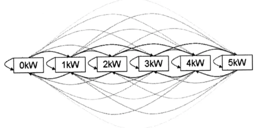
It is straightforward to represent wind data with Markov chains: each state is a wind speed [m/s] or a wind power [kW], and from any given speed/power, there is some probability distribution function of what the next speed/power will be.
Figure 2-1: A simple first-order Markov chain for wind power modeling
2.2.1
Mathematical Description
At its core, a Markov chain is a sequence of random variables (W1, W2, W3, ...) such
that future states (Wn+1, W.+2, ...) are dependent only upon the current state Wn
and are independent of all past states (W1, W2, ..., Wn-1).
Wn = Wjlwj E {w, W2, ... , WK-1, WK} (2.1)
Where {wl, w2,..., K-, WK} is the set of K discretized wind speeds or wind powers.
The transition probabilities between states can be represented by a transition matrix P such that the element pij is the probability of transitioning from state i to state j. Formally,
Pij = P (Wn+1= WjlWn = w) (2.2)
Since the transition probabilities from a given state must add to 1, it must be true that
(2.3)
-'Pid = 1
2.2.2
Higher Order Markov Chains
Though memoryless by mathematical definition since the current state solely
deter-mines the transition probability distribution, Markov chains can be created to have multiple time step memories. For a first order chain, each state represents a wind power value for a single time period, but it is possible to create an N-order Markov chain where each state is defined by a set of N wind powers. For example, a third order model (N = 3) would include states with three elements: {fn-2, Wn-1,
where wn is the value of the wind power at time step n. In this higher order case,
the next state's {wn-2, wn-} must equal the current state's {wn-1, wn}. The problem with higher order Markov models is that there are KN states, where K is the number of discretized wind powers and N is the order of the model, which is intractable for large N.
2.3
Using Markov Chains to Model Wind
In much literature, Markov chains have been proposed as a reasonably acceptable generator of synthetic wind speed data. Authors have used various transition matrix sizes, various time steps, and various orders:
* Jones et al. 1986 - Uses first-order 11 x 11 transition matrix for eight-hour means [19].
* Kaminsky et al. 1991 -Uses first-order and second-order 21 wind speed Markov chain at 3.5Hz. Correctly points out that the Markov model does not contain enough low-frequency data [20].
* Sahin et al. 2001- Uses first order 8 x 8 transition matrix for hourly time steps. States second and even third order autocorrelation coefficients are significant, and suggests higher order transition matrices for future work [33].
* Ettoumi et al. 2003 - Uses a highly discretized (3 x 3) Markov transition matrix for three-hour increments. Notes that measurements performed at h-6, h-9 are
non-negligible [14].
* Nfaoui et al. 2004 - Uses first-order 12 x 12 transition matrix for hourly means
[28].
* Shamshad et al. 2005 -Uses first and second-order Markov chains with 12 wind speeds for hourly means. This paper notes the autocorrelation plots are a poor match [35].
* Papaefthymiou et al. 2008 - Uses 35-state first through third-order Markov chains for 30-minute intervals [31].
For this study, Markov chains of various orders, various numbers of states, and various time steps were trained using months of high resolution power data from a 1kW wind turbine donated by a utility wishing to remain anonymous. These Markov chains were then used to generate synthetic wind data. Although the probability distribution of the wind power was correct in each model, the generated synthetic data often lacked other characteristics of the original data. In particular, time evolution characteristics of the wind data characterized by autocorrelation plots of synthetic wind speeds or wind powers generated by Markov chains are often very different
from the original data, especially for models with short time steps. Modeling wind with especially short time steps is vital for microgrid simulations, since microgrids have much lower inertia than larger grids, and will require agile automatic generation control or storage control. Additionally, power cannot be supplied to an islanded microgrid from elsewhere, so it is critical that the storage or backup generation be sized correctly.
2.3.1
Markov Chain Creation
The continuous spectrum of wind power levels must be discretized into K states.
Begin with a zero matrix M of length equal to K, the number of discrete wind power states, and of dimension equal to one plus the order of the model. For example,
a second order model with 32 discretized wind powers would begin with a zero matrix
M of dimensions 32 x 32 x 32.
Step through the real data, incrementing the "tally matrix" M. For example, if
the wind power is wi at time step n - 2, wj at time step n - 1, and Wk at time step
n, then mijk would be incremented.
The probabilities for state transitions are calculated from the frequency of tran-sitions, so it is necessary to normalize the matrix M into a probability transition matrix P. Each row of M along the highest dimension is divided by the sum of that row. Effectively, each highest dimension row then adds to 1, and is a valid probability mass function (PMF).
The transition matrix can then be used to simulate time series data. Given a number of "seed" wind powers equal to the order of the model, the matrix provides a PMF of what the next wind power will be. Using a random number generator in
conjunction with the appropriate PMF from the matrix, the next wind power, wn+l, is chosen. The process is continued indefinitely using the recently generated wind power states as inputs to the matrix to find the PMF of the next wind power.
2.3.2
Wind Speed or Wind Power?
Markov chains can be used to represent either wind speed or wind power. Many of the mentioned studies model wind speed instead of wind power. Luckily, it is straightforward to convert a wind speed Markov chain to a turbine power output Markov chain. The power contained in the wind is proportional to the velocity cubed:
Wind turbines have a minimum cut-in speed, a maximum power output, and a cut-out speed, which can all be incorporated using the function:
0 if v < Vcutin
Cv3 if vcutin < v < Pmax/C (2.5)
P = (2.5)
Pmax if /PmaxC < v < vctout 0 if Vcutout _ v
Where C, Pcutin, Pmax, and Pcutout are all properties of the wind turbine. Real wind
turbine power curves will not follow this exact theoretical curve since mechanical losses increase at higher wind speeds.
2.3.3
Appeal of Markovian Wind
Markov chains are intuitively appealing for modeling wind because given the current wind speed or power, one can guess the possibilities for the value a short while later: it will probably be slightly windier, slightly less windy, or about the same. Markov chains are able to model this because from every state, there is a set of probabilities of transitions to other states. The output of Markovian wind models are a giant improvement over a simple Monte Carlo approach with no temporal correlation.
A less intuitive appeal of Markov chains is that they nearly perfectly reproduce the PDF of the original data. What follows is a proof for the first order case.
Recall the "tally matrix" M from Section 2.3. In stepping through the data, the transition from wn-1 = wi to w, = wj is tallied by incrementing mij, and then the transition from w,, = wj to w,, = Wk is tallied by incrementing mjk, and so on. So
row j and column j of matrix M are both incremented because the wind transitioned to state j on one time step, and then from state j on the next time step. Also note that if the wind power remains the same for consecutive time steps (w-1 = wj and
wn = wj), mjj is incremented, and still both row j and column j of matrix M are
row and the column, but for large amounts of input data, the effect of these two individual data is diminished. Hence, for a large amount of input data,
(2.6)
Smij
mij ? i Define ci and cj as i = mij Cj = Zmij (2.7) (2.8) From Equation 2.6, ci Cj (2.9)Since row i of matrix M is tallied for every wind power state transition from state
i, the observed distribution from the real data is the Ci
7ri
-zci (2.10)
Next, it is shown that 7r of the actual data matches the stationary distribution
of the simulated data, referred to as fr. Recall transition matrix P is a normalized version of M, so each element of M must be divided by its row's sum, ci.
Pij = mij/ci PijCi
ZPij
Cj =mij = mij = cj (2.11) (2.12) (2.13)Substituting from Equation 2.9, one finds that CT is a left Eigenvector of P.
SPij
Ci cii
CT , CT p
(2.14)
The stationary probabilities of the Markov simulation, tr,[6] are also the left Eigen-vector of P with Eigenvalue of 1, such that
77 = rP (2.16)
So CT is approximately a scaled version of fr. fr is already scaled to sum to 1. Equation 2.10 defines 7r as CT but scaled to sum to 1. Since 7 is a unique solution to the stationary distribution of irreducible, aperiodic, recurrent Markov chains,
7r - r (2.17)
2.4
Results
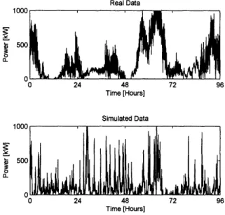
The difference between real data and synthetic data generated by a Markov chain using an overly short time step is clearly visible in Figure 2-2. This synthetic data
'C a Real Data Time [Hours] Simulated Data t nnn o 500 0 a. 24 48 Time [Hours] 72 96
Figure 2-2: Markov chains at small time steps clearly differ from the original data
was generated from a first order Markov model with a time step of 1 minute that was constructed from the historical data above it. As shown by the proof in Section 2.3.3, this synthetic data has the same PMF as the real time series data. However, the
1I~A~A
-simulated data lacks the persistence of the historical data and would clearly predict a radically different storage requirement for the system.
2.4.1
Autocorrelation
Autocorrelation is a good metric for the dynamics of time series data, and it is used
to analyze this Markov model. The autocorrelation function is calculated by
R[j] =
i-j
k=l
(2.18)
where c is the mean of
correlation between one
0.2
0
-0.2
-0
w [9]. Conceptually, the autocorrelation is a measure of the
data point and another that is j time steps ahead or behind
Autocorrelation: 5 Minute Sampling, 20 Wind Power Levels
- Original Data
- -. First Order Simulated Data
- - - Second Order Simulated Data
- - - Third Order Simulated Data
24 Time [hours] Figure 2-3: wind power Autocorrelation levels)
coefficients are too small at 5-minute time steps. (20
The autocorrelation of synthetic data drops off too quickly when short time steps are used, as shown in Figure 2-3. Clearly, the problem is worse for first order Markov chains than it is for higher-order ones. The reason for the steep decline of the first order model is that even if current wind is affected by the wind five minutes ago, it
c
--has little to do with the wind several hours earlier.
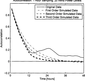
Autocorrelation: 1 Hour Sampling, 20 Wind Power Levels
---- Original Data
- - First Order Simulated Data
0.8. - -- Second Order Simulated Data
- - -Third Order Simulated Data
0.6 -C 0.4 0.2--0.2 0 12 24 36 48 Time [hours]
Figure 2-4: Surprisingly, autocorrelation coefficients can be too large at longer time steps. (Hourly time steps, 20 wind power levels)
Interestingly, the autocorrelation for short lags under 12 hours is too large when longer time steps are used, as is shown in Figure 2-4. Here the third order Markov chain does a better job of mimicking the early curve of the actual autocorrelation data.
In both cases, the third order model is generally better at replicating the original data than the first or second order models. Because the size of transition matrices
is K(N+I) where K is the number of wind powers and N is order, orders higher than
N = 3 were not tried.
Since Markov chains have only a short order/memory (one to three time steps in this study), it is impossible to model daily trends with time steps shorter than several hours. The local maximum around 24 hours in Figure 2-3 and Figure 2-4 occurs because afternoons are typically windier than mornings or nights at this wind turbine's location. As a result, the model is not valid for producing time series data for longer lengths of time. Interestingly, the first order model in Figure 2-4 is actually a better match in the hourly case if the averaging occurs over 24 hours because of its abnormally high autocorrelation, which passes through the daily local maximum of
the real data.
2.4.2
Autocorrelation Error
In order to clearly determine the effect of various Markov chain parameters on the au-tocorrelation, a metric was developed for judging the accuracy of the autocorrelation function of the synthetic data: the RMS error of the autocorrelation values between 0 and 12 hours. Formally,
E = T (2.19)
where T is the number of time steps in the 12-hour window and R is the autocorre-lation data.
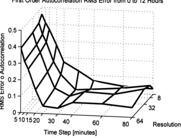
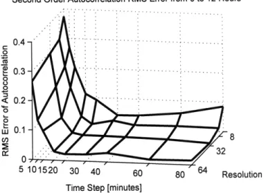
Figure 2-5, Figure 2-6, and Figure 2-7 display error as a function of time step and wind power resolution (the number of discrete wind power states) for first, second, and third order Markov models.
First Order Autocorrelation RMS Error from 0 to 12 Hours ... ... 0.5 . 0.3 S0.2 o 0.1 O.. 32 5101520 30 40 6(
Time Step [minutes]
80 64 Resolution
Figure 2-5: First Order Autocorrelation Error
The important result is that higher order models reproduced the autocorrelation characteristics of real data down to the lower time step limit of 15 minutes.
Second Order Autocorrelation RMS Error from 0 to 12 Hours 0.4 -C " 0.3-3 0 < 0.2Uij 0.1 -C/ 8
/
32
5 101520 30 40 60 80 64 ResolutionTime Step [minutes]
Figure 2-6: Second Order Autocorrelation Error
Third Order Autocorrelation RMS Error from 0 to 12 Hours
c 0.3 ... .... .3 2 <0. -0 6 5101520 30 40 60 80 Resolution
Time Step [minutes]
Figure 2-7: Third Order Autocorrelation Error
In Figure 2-5, the 80-minute model with eight wind states has less error than the model with 16. Also, small time steps are obviously inaccurate, but steps larger than an hour are not necessarily optimal, either. This is shown in Figure 2-6, where the 8-state, 80-minute Markov model has more error than the 8-state 30-minute Markov model. Despite these exceptions, it is fairly clear that the best model is the third order model with many wind power states.
2.5
Why Markov Wind Models Are Dangerous
Dynamic wind data has multiple applications, including reliability studies as well as sizing storage and spinning reserve for grids with a high penetration of wind power. In order to determine whether or not the accuracy of the model actually matters, a simplified storage simulation was created.
2.5.1
Underestimated Storage
A hypothetical situation was modeled, in which a purely wind-powered microgrid was islanded for 12 hours. It is assumed that the average power generated by the wind model during this period perfectly matches the microgrid's perfectly flat load
profile. The storage required by this situation was calculated by first integrating the generation minus the load to yield the energy stored as a function of time. Then the
storage size was determined by subtracting the minimum energy from the maximum energy. Using the storage necessary to cover the worst case would have been highly susceptible to outliers, so the 95% tile was used instead-the amount of storage that would be able to supply the load in 95% of cases. This process was tried on both real and synthetic data. The synthetic storage values were then divided by the real
storage value, yielding a storage fraction where 1 is a perfect estimate.
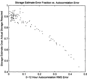
Figure 2-8 is a plot of the storage fraction and the RMS error of the autocor-relation. Interestingly, all models underestimated the amount of storage necessary. Clearly the models with a low 12-hour autocorrelation RMS error yielded more accu-rate storage estimates. The higher error models grossly underestimated the storage
necessary.
2.5.2
Not Accurate for FAPER Simulations
Markov models, while properly reflecting the probability density function of wind data, are not necessarily appropriate in generating synthetic data for simulations in which time evolution of the data is important for determining artifacts such as the need for storage. This is particularly true for short simulation time steps. While
Storage Estimate Error Fraction vs. Autocorrelation Error • -0.9 ,. . 0 0.8-1 < 0.7 0.6 0.5 0.4 0 0.1 0.2 0.3 0.4 0.5
0-12 Hour Autocorrelation RMS Error
Figure 2-8: Storage estimates and RMS error are strongly correlated.
this study used anecdotal data from a single turbine, it was determined that the limit was about fifteen minutes. Even well-fitted Markov models cause simulations
to underestimate energy storage requirements.
New methods need to be developed for the generation of short time step synthetic
wind speeds and powers-methods that can replicate an autocorrelation function while simultaneously retaining the correct probability distribution of the original data. ARMA models have been used in the literature, but these do not necessarily retain the probability distribution of the original data. Further study is also needed for large wind farms with many turbines, which will likely have smoother characteristics. For the remainder of this thesis, real wind power data was used to ensure correct autocorrelation.
Chapter 3
Microgrid Model and Simulation
3.1
What is a Microgrid?
Generally, a microgrid is a small power grid. The exact size of grid denoted by the term "microgrid" is the cause of much debate. Microgrids might be low voltage (LV), usually below 1kV, or medium voltage (MV), usually between 1kV and 69kV [17]. The amount of power on a microgrid is typically around 2MW, but theoretically a
microgrids could be as small as a few houses (10kW) or as large as an entire college
campus (over 20MW). Isolated microgrids have existed since the days of Tesla and Edison, but the interconnected microgrid concept has recently garnered attention because small partitions of the grid might intentionally "island" from the main grid
and weather a large-scale blackout.
Today in large systems, an outage on a transmission system unequivocally causes
outages on the distribution systems connected to that transmission system. One reason for this is that a tremendous amount of local generation would be required to provide enough power for the local load on a distribution system. While DG is still a small fraction of generation today, the increased penetration of distributed re-newables through incentives such as California's Million Solar Roofs Plan may shift this paradigm [30]. More important than the present low penetration, however, is the precaution on behalf of the power grid repair team-it would be an unpleasant surprise if part of a downed system were still, in fact, energized. Modern day
dis-tributed generators, such as grid-connected solar roofs, are equipped with various anti-islanding schemes to ensure that they disconnect from the local grid in the event of an upstream disconnect from the main grid [11]. Basic anti-islanding techniques
include monitoring for frequency and voltage drifts, and more advanced active tech-niques include intentional variations from a 50/60Hz sine wave, which would impact the stability of islanded grids triggering the unit to disconnect [40].
Recently there has been a trend towards increased penetration of distributed gen-eration. For example, in Ota, Japan, there were 550 of rooftop solar installations in a half square kilometer area of the city at the end of 2005 [18]. Intentionally islanding part of the grid in a blackout would increase reliability for the users on that islanded grid. Current thought on microgrids implies that a distribution system might be its own islanded microgrid. This is a logical choice because distribution systems (unlike transmission systems) are typically radial in nature, so it is relatively easy to define a single primary connection point to the medium or high voltage grid.
The chief control strategy of microgrids is known as "single master" or "master slave." In this configuration, most DGs are set to current mode, and a single "master" is responsible for keeping voltage and frequency at their target values. This master DG may or may not also direct other DGs to start, stop, or even change set points, hence the name "master slave." An alternate configuration includes multiple master DGs, appropriately named, "multi-master" control. Both control methods generally use frequency droop control, so power output is a function of grid frequency [26].
On large grids like the Western or Eastern Interconnect, second-to-second varia-tions in load are extremely small compared to the amount of power being consumed because of the law of large numbers. Islanded microgrids will have a much higher per unit fluctuation in load so the frequency and voltage will not be as stiff. On such microgrids, a great deal of load-following will be necessary, hence the reason for this study. Automatic generation control (AGC) is a function of both interconnection power flow measurements and grid frequency, so FAPERs can provide services on full-sized grids as well [12].
Sometimes a distribution system is at the end of a undersized transmission line that
becomes a bottleneck during periods of high load. This problem cannot be sensed purely through the voltage or frequency at the outlet-it is an issue the ISO or RTO must sense and correct with load shedding or DG in the critical area. Besides, FAPERs perform load adding and shedding to balance generation/load on a shorter time step (minutes) than would be necessary for reducing line flows all afternoon on a hot day (hours). Other demand response technologies such as dishwashers or laundry
machines that can wait for hours are better solutions than FAPERs for this problem.
3.2
Simulated Microgrid
For this study, many iterations of lengthy simulations were required to test the
vir-tual appliances. The simulations are calculation-intensive for a two reasons. First, simulation time steps on the order of 100ms are required for accurate grid frequency
calculations, yet appliances have cycle times of up to an hour, requiring long simula-tions with short time steps. Second, "bang-bang" (on-off) appliance logic dictates 500 Boolean decisions be made each iteration of an ordinary differential equation solver, which is inherently more conducive to continuous functions than discrete functions. For these reasons, the simplest microgrid is modeled (Figure 3-1): there are no power lines and no reactive power. The simplification was necessary for simulation efficiency, but can be rationalized as follows:
* Distribution systems are geographically dense, so power lines are short and therefore less inductive.
* FAPER appliances are in houses distributed throughout the microgrid, so heavy loading of individual lines on the microgrid should not occur.
When FAPER load shedding occurs, inductive compressors in cooling appliances will be turned off so the voltage of the distribution system is necessarily likely to rise slightly. The impact of demand response on system voltage is suggested at a future area of research.
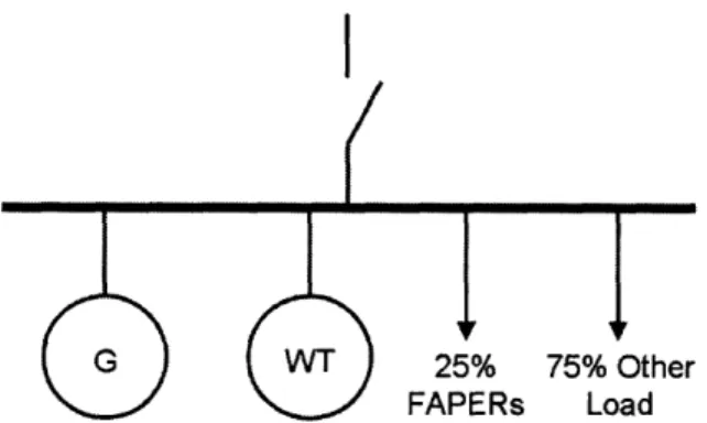
G WT 25% 75% Other
FAPERs Load
Figure 3-1: A simple microgrid was used for simulations. The key equation relating power to grid frequency is the following [22]:
2H dw Pin - Pout
(3.1)
wo dt PB
This is implemented in Appendix B in Figure B-4.
It has been argued that inverters have no inertia, and that power on inverter-based microgrids will be correlated to voltage instead of frequency. While the natural
effect on overloaded power electronics is a voltage drop, voltage source inverters can be controlled to behave like synchronous machines [8][15][24]. The relevance to this study is that frequency-droop control will likely be used for microgrid control, so frequency-responsive FAPERs will work on the system.
It was shown in Chapter 2 that traditional wind power modeling tools are unable to reproduce realistic wind speed trends at short time steps. Accordingly, the code in Section A.1.1 was used to extract real wind and real load data, both donated by
a utility wishing to remain anonymous. This code is necessary to convert the dead band-recorded data, which was recorded each time a value exceeded bounds around the previously recorded value, into data with a regular time step.
3.2.1
Simulation Description
The wind turbine and load data are fed to the code in Section B.1.1, which initializes and runs the Simulink model below in Figure 3-3. A simplified version of the Simulink model is displayed in Figure 3-2
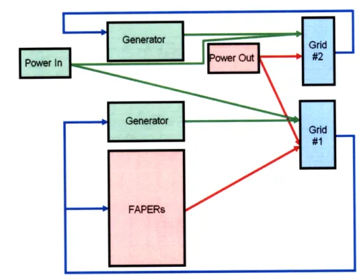
Figure 3-2: Simplified Simulation Block Diagram: Green lines indicate generation, red lines indicated load, and blue lines indicate frequency.
The sub-blocks in Figure 3-3 can be found in Section B.2. The Simulink model contains both an experimental grid and a control grid (Grid 1 and Grid 2). Both have identical frequency-droop generators and both are fed the same inputs, except that a portion of the experimental group's load is FAPER load rather than the load data. The color scheme and layout for the Simulink diagram is the same as the simplified diagram in Figure 3-2. Many of the miscellaneous white blocks are gain calculations.
For this simulation, the penetration of wind is 25%, meaning 25% of the energy comes from wind over the course of the simulation (as opposed to capacity). 25% penetration was chosen because beyond this penetration, serious storage is required. Except for Maine, states with renewable portfolio standards typically have goals of 25% or less. Minnesota, Oregon, and Illinois all have the ambitious goal of 25% renewable energy by 2025.
Droop gains for the frequency-droop controlled generators were simply increased until the grid frequency range of the control grid (without FAPERs) remained within
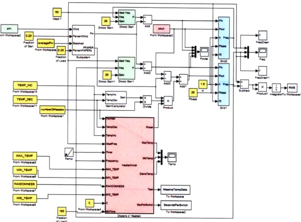
of Lod
Figure 3-3: Full Simulation Block Diagram: Green blocks are generation, red blocks are load, blue blocks are the grids, yellow blocks are inputs, grey blocks are outputs, and white blocks are miscellaneous.
about 0.1Hz. Chapter 4 contains more details about the FAPER part of the simula-tion.
Chapter 4
FAPER Model
As described in Chapter 1, the FAPER concept is to turn people's temperature-bounded appliances into energy storage using grid frequency as a signal. FAPERs act as load and generation shedding: they turn off when there is a power shortage (low frequency) and on when there is a energy surplus (high frequency). They also act as energy storage because extra cooling or heating occurs during high frequency periods so the units can essentially ride through low frequency periods on the heat/coolness
that they already have.
FAPERs are chosen over "Voltage Adaptive Power and Energy Reschedulers" (VAPERs) because voltage is a poor indicator of the generation-load balance. Low voltage can be solved by adding reactive power to the system or by changing a tap changer setting. Locally, low voltage may occur when a high-current device (e.g. a vacuum) turns on and causes a voltage drop across household electrical lines.
4.1
Linear Approximation of Appliance Behavior
The cooling appliance model proposed in Constantopoulos et al. in 1991 is the fol-lowing [10]:
T is the cooling compartment temperature at time ti, E is the system inertia, and
depends on the insulation A, the thermal mass inside the appliance me, and the time span 7 between the two time points ti and ti+l. Parameter qj denotes the electrical power required when the device is on; effectively this will be a square wave. 'q is the efficiency of the cooling device, and To describes the ambient temperature.
This function can be approximated by a (linear) triangular wave when the co-efficient converting energy into power does not change much from the beginning of the cooling cycle to the end, and when the warming coefficient does not change much from the beginning of the warming cycle to the end. In other words, letting
ATi = max {T)} - min {T}:
AT << TO - Ti (4.2)
AT, << T - T o - A (4.3)
Intuitively, more heat seeps into an ice box when the temperature is very different between the inside of the fridge and the outside. That difference does not change much, though: room temperature is roughly 22 degrees C and refrigerators oscillate
between 1.5 and 3.5 degrees C, so the change in fridge temperature is very small compared to the difference between the fridge and the outside (AT = 2 and T - T =
19.5). Additionally, a 50% duty cycle means that n1 = 2 (TO - T), so
ATs << T - To - 7 )
AT << T (To - 2 To - T) (4.4)
AT << TO - T, which we know is true
In conclusion, the linear triangular wave used to model appliance temperatures is a good approximation of real appliance behavior.
4.2
FAPER-capable Appliances
Figure 4-1 details which appliances can be easily turned into FAPERs. The following subsections describe the behaviors of various appliances and how they might be made into FAPERs.
Percent of Total Electricity Consumption in US Housing Units, 2001
Refrigerators and Freezers 14% Other 32% Air Conditioners and Electric Heaters TV 22% 2%
Electric Hot Water Range Heaters
4% 8%
Furnace Fan 7% Clothes
3% Pool Heaters Dryers and 1% Dish
Washers
Figure 4-1: Household Electricity Consumption Makeup [1]. The complete data can be found in Appendix C
4.2.1
Refrigerators and Freezers
Refrigerators and freezers make up 17.2% of residential load [5]. They are excellent candidates for FAPERs and have been the focus of several dynamic demand papers
[37] [38].
One study assumes that refrigerators and freezers stay on for 10 to 30 minutes at a 50% duty [29]. A different study assumes a distribution where the mean on time for refrigerators is 30 minutes and the mean off time is 103 minutes [38]. In a statistically insignificant number of trials, it was concluded that the first study by Nipkow in 2002
more closely represents typical appliances.
In discussions with an expert in refrigeration cycle analysis, it was determined that restarting a compressor within about 3 minutes of shutting it off may cause mechanical problems since pressures may have not equalized [4]. While relatively benign to the physical components, short cycling, the act of stopping the compressor cycle early, reduces the efficiency of the appliance [2]. A tradeoff must be made between decreasing cycle times and increased FAPER effectiveness. This tradeoff is explored in Chapter 5.
4.2.2
Air Conditioners and Electric Heaters
Space heating and cooling comprises 26.1% of residential load [5]. Air conditioners and heaters are other excellent opportunities for implementing FAPER technology. Unfortunately, the duty cycle times of air conditioning systems are largely undoc-umented. One reason for this is the highly variable setups: air conditioners range from small window units to giant central units. Because of the lack of data, this
study assumes they have similar characteristics to refrigeration cycle times. This is a worst-case scenario, since it increases the odds of uniform grouping explored in Section 5.2.
4.2.3
Hot Water Heaters, Clothes Driers, and Dish Washers
Hot water heaters are 9.1% of residential load, and clothes driers and dish washers make up 8.3% of residential load [5]. Electric hot water heaters are sporadic in their energy use: they do most of their heating while the resident is bathing/showering or while other appliances use hot water.
Though hot water heaters do keep a temperature between two bounds, they are not ideal candidate for FAPERs as described in this thesis since the user would likely notice the curtailment. Because of the high power usage however, these appliances are good candidates for helping in emergency situations. Pacific Northwest National Laboratory ran a study in which hot water heaters and clothes driers turn off for a
brief time when the frequency drops to an emergency threshold [23]. This emergency
operation mode is fundamentally different from the constant delicate balancing of frequency by a large group of FAPERs explored in this thesis. Nonetheless, it is clear from the PNNL study that appliances such as these can aid in frequency regulation.
4.2.4
Pool Heaters
Pool heaters make up only 0.9% of residential load [5]. Despite the small percent of total load, pool heaters are ideal FAPER candidates because of the high power draw per device and the regularity of the cycling (unlike typical hot water heaters). Additionally, the thermal mass of most pools is large compared to refrigerators, and
pool temperatures are non-critical, so the delay of heating is unlikely to be noticed by users.
4.2.5
Shorten Time to Hibernate
The concept of shedding load based on frequency is not restricted to temperature bounded appliances. One application might involve a computer that switches to hibernate mode on low frequency if it has been inactive for some period of time. Or, since lighting is 8.8% of load [5], motion detectors could be combined with frequency sensors to turn off lights in empty rooms on low frequency.
Proximity sensor lights and other hibernating appliances cause a conflict of interest between energy efficiency and FAPER technology. If it has been decided that no one
is in the room, the energy saved by shutting the appliance off immediately is likely more profitable to the consumer than any payment they would get for the ancillary
service that FAPERs would provide.
4.2.6
Plug-in Hybrid Electric Vehicles
One study estimates the market share of plug-in hybrid electric vehicles (PHEVs) will reach 25% by the year 2020 [16]. PHEVs are in a unique position, along with dishwashers, to aid both economic dispatch and regulation: they can wait until the
middle of the night to charge, and then while they are charging they can "stutter" their power usage to help regulate the grid [21]. Since PHEVs have very different characteristics than typical FAPER appliances, and since they have not penetrated markets yet, they are not modeled in this study. Nonetheless, one day electric vehicles may play a role in providing ancillary services for the power grid.
4.3
FAPER Simulation Setup
For this study, electric heating, air conditioning, and refrigeration are lumped into one group of loads. The cycle times of these appliances are roughly similar, where on times are typically over 10 minutes and complete cycle times are generally under one
hour. Since appliances on microgrids would not be identical, the heating and cooling time are randomized in the simulation using the following code:
Randomnessl = 1/TempInc* ...
(1 + RANDOMNESS*(1-2*rand(size(HeatArray)))); Randomnessl = Randomnessl. ^(-1) - TempInc;
Randomness2 = 1/TempDec* ...
(1 + RANDOMNESS*(1-2*rand(size(HeatArray))));
Dec = Randomness2. ^ (-1);
IncMinusDec = TempInc+Randomnessl-Dec;
where RANDOMNESS determines the amount of randomness among appliances, Dec is
moff, and IncMinusDec is mon - moff.
The inverse of the slopes 1/mon and 1/mff are uniformly distributed, centered around the ideal 1/mon and 1/moff that cause a cycle time similar to those found in the literature [29]. Effectively, the on and off times are both uniformly distributed in this study from 10 minutes to 30 minutes. mon and moff are uncorrelated, and it can be shown that the average on time in this "varied appliance" case is still 50%:
Letting mon and moff vary from mo - Am to mo + Am
1 jmo+Am Mmo+Am mo dmof fdo
S dmoffdmn o dmffdm
4Am2 Jmo-Am Jmo-Am mon+ moff
1 mo+Am mon mon mo
4Am2 fmo-Am mo-Am mon + moff f off mon
= (1)dmof fdmon
4Am2 mo-Am 1
mo-Am
1 /mo+Am
4A 2 o-Am (mon - (mo0 - Am)) dmon
4Am2 > (4.5) (4.6) (4.7) (4.8) (4.9)
500 units with identical peak power consumption (as opposed to average power consumption) were chosen as the result of a tradeoff between smoothed group behavior
and fast simulation time. Simulations containing fewer appliances owed too much of their behavior to individual appliances in the system. More than 500 appliances did not significantly change simulation results but greatly slowed the processing time.
The temperatures of the appliances are normalized on a scale of 0 to 1. When the
appliances are on they tend towards 1 at predefined slope mon, and when they are off they tend towards 0 at slope moff. In other words, heaters' hottest temperatures are 1, and cooling appliances coldest temperatures are 1. The minimum appliance off
time was limited to 180 seconds, so that cooling appliances' compressors would not be damaged by leftover pressure from previous cycles.
Special attention was paid to the initial state of the appliances. The temperature bounds at 60Hz are calculated and appliances are distributed randomly across the window with the appropriate fraction turned on. For an average duty cycle of 50%, simply half of the units are on at the beginning of the simulation.
By constructing the set of 500 digital appliances as described in this chapter, paired with the microgrid of Chapter 3, a complete simulation is formed, the results of which are discussed in the following chapter.
Chapter 5
Insights to Optimal FAPER
Control
This chapter discusses various FAPER control schemes. First a literature survey is
conducted, and then a new probabilistic algorithm is described and its parameters are optimized using a Monte Carlo approach.
5.1
Literature Survey
* Homeostatic Utility Control [34]
This is the first article to suggest frequency adaptive loads. The article, by
Schweppe et al., gives an example of an industrial melt pot: a giant load re-sponsible for keeping a metal's temperature between two bounds. Schweppe et al. note the difference between governor function and spinning reserve. In one embodiment, the loads constantly balance the frequency. In another embod-iment, the loads trigger only on extreme frequency fluctuations. It is argued that FAPERs could eliminate the need for AGC, leaving generators responsible for 5 minute adjustments, not constant adjustments.
The algorithm proposed by Schweppe, et al. includes changing temperature bounds: high frequency increases the minimum temperature bound of heaters,
Temperature
Frequency
Figure 5-1: The Control Function in Homeostatic Utility Control [34]
causing many units to turn on and heat, whereas low frequency decreases the upper bound, forcing many units to turn off and cool.
* Stabilization of Grid Frequency through Dynamic Demand Control [37]
This article, by Short et al., includes a relatively detailed model of refrigerators and a simple FAPER (called DDC: dynamic demand control) algorithm, shown in Figure 5-2. The paper details the improved system response to a sudden loss of generation.
This control method differs from the one in Figure 5-1 because in normal op-eration (e.g. the center frequency where f = 60Hz) the temperature limits are somewhat restricted. The advantage of this is that the power response to a fre-quency change is potentially increased: for example, on a frefre-quency rise, both more units turn on and fewer units turn off. In Figure 5-1, only more units turn on-the number of units turning off is not affected. The disadvantage of this control method is that the cycles of appliances are decreased, potentially reducing the life of the appliance.
* Demand-based Frequency Control for Distributed Generation [7]
This article by Black, et al., suggests that FAPERs (called DBFC devices: de-mand based frequency control devices) sample grid frequency at regular intervals and respond only when the frequency deviates from a predetermined window. The benefit of this approach is that the sampling times guarantee a temporally distributed response.
Temperature
Teprtr
A
I
Frequency
Figure 5-2: The Control Function in Stabilization of Grid Frequency Through
Dy-namic Demand Control [37]
Design Considerations for Frequency Responsive Grid FriendlyTMAppliances
[27]
This article examines WECC frequency data and examines what control pa-rameters might be used for FAPERs (called FR-GFAs: frequency responsive Grid Friendly AppliancesTM). The paper focuses on under-frequency events: the authors, Lu at al., define a minimum grid frequency, which must be ex-ceeded for a predefined triggering delay, for the unit to shut off. A reset delay is also discussed to avoid responding chaotically to frequency oscillations.
5.2
Observations and Insights into FAPER
Con-trol
In the control algorithm presented in [34] and [37], temperature limits vary directly with frequency. In simulations, this had the potential to cause three major problems. First, high gains can result in an unstable system. A rise in frequency causes too many FAPERs to turn on, which overloads the system, causing a drop in frequency, which causes even more FAPERs to turn off, which causes an even sharper drop in load and hence a larger frequency rise etc. This behavior can be seen on the left side of Figure 5-3.
Second, when the frequency swings both high and low within a short duration of time, FAPERs as a group become unresponsive because the hottest units are already cooling and the coldest units are already heating. Slightly shifting the temperature