Publisher’s version / Version de l'éditeur: Technical Report, 2012-11-01
READ THESE TERMS AND CONDITIONS CAREFULLY BEFORE USING THIS WEBSITE.
https://nrc-publications.canada.ca/eng/copyright
Vous avez des questions? Nous pouvons vous aider. Pour communiquer directement avec un auteur, consultez la première page de la revue dans laquelle son article a été publié afin de trouver ses coordonnées. Si vous n’arrivez pas à les repérer, communiquez avec nous à [email protected].
Questions? Contact the NRC Publications Archive team at
[email protected]. If you wish to email the authors directly, please see the first page of the publication for their contact information.
NRC Publications Archive
Archives des publications du CNRC
For the publisher’s version, please access the DOI link below./ Pour consulter la version de l’éditeur, utilisez le lien DOI ci-dessous.
https://doi.org/10.4224/21263086
Access and use of this website and the material on it are subject to the Terms and Conditions set forth at
Correlation of model-scale to full-scale ice piece size
Lau, Michael; Wang, Jungyong; Seo, Dongcheol; NRC Ocean, Coastal and River Engineering
https://publications-cnrc.canada.ca/fra/droits
L’accès à ce site Web et l’utilisation de son contenu sont assujettis aux conditions présentées dans le site LISEZ CES CONDITIONS ATTENTIVEMENT AVANT D’UTILISER CE SITE WEB.
NRC Publications Record / Notice d'Archives des publications de CNRC:
https://nrc-publications.canada.ca/eng/view/object/?id=8d2bad29-7115-49ab-8a35-9436569b7696 https://publications-cnrc.canada.ca/fra/voir/objet/?id=8d2bad29-7115-49ab-8a35-9436569b7696
Report Documentation Page REPORT NUMBER OCRE-TR-2012-30 PROJECT NUMBER A1-00765 DATE November 2012
REPORT SECURITY CLASSIFICATION
Unclassified
DISTRIBUTION
Unlimited
TITLE
CORRELATION OF MODEL-SCALE TO FULL-SCALE ICE PIECE SIZE
AUTHOR(S)
Michael Lau, Jungyong Wang and Dongcheol Seo
CORPORATE AUTHOR(S)/PERFORMING AGENCY(S)
NRC Ocean, Coastal and River Engineering – St. John’s, NL
PUBLICATION
SPONSORING AGENCY(S)
Canadian Coast Guard
RAW DATA STORAGE LOCATION(S) PEER REVIEWED
MODEL # PROP # EMBARGO PERIOD PROJECT A1-00765 GROUP Research PROGRAM Arctic Operations FACILITY Ice Tank KEY WORDS
Model Test, Sea Trial, Correlation, Polar Icebreaker, Piece Size PAGES iv, 20 FIGS. 14 TABLES 6 SUMMARY
This document summarizes the model-scale to full-scale ice piece size correlation performed at the National Research Council’s Ocean, Coastal, and River Engineering (NRC-OCRE) St. John’s Ice Tank. This correlation work supports the NRC-OCRE CCGS Polar Icebreaker model test program; it is based on an earlier investigation by Lau et al (1999) on the influence of ice thickness on piece size during icebreaking by sloping structures. For this study, additional data from the CCGS R-Class icebreakers and the USCGC icebreakers Healy and Polar-Star are examined. The study is focused on the scaling performance of NRC-OCRE EG/AD/S model ice with respect to piece size generation. This study has shown the non-dimensional piece size decreases and approaches that found in full scale beyond a certain thickness, i.e., ~ 9 cm. We tested the Polar Icebreaker model in EG/AD/S model ice at 8 cm and 10.4 cm, and at this range we expect the similar thickness
dependency follows. However, the bow breaking pattern of the Polar icebreaker model produced much larger pieces in comparison with other more conventional icebreaking bows, i.e., the R-Class, tested in similar ice thickness. It points to a need for further assessment of the bow shape influence on broken piece size, as the Polar icebreaker designs have bow geometry significantly diverse from the traditional icebreaker bow forms that may contribute to different icebreaking patterns and hence piece size.
ADDRESSES:
NRC - Ocean, Coastal and River Engineering St. John's
Arctic Avenue, P. O. Box 12093, St. John's, NL A1B 3T5
Ottawa
1200 Montreal Road, Building M-32 Ottawa, Ontario K1A 0R6
National Research Council Canada
Ocean, Coastal and River Engineering
Conseil national de recherches Canada
Génie océanique, côtier et fluvial
CORRELATION OF MODEL-SCALE TO FULL-SCALE ICE PIECE
SIZE
OCRE-TR-2012-30
Michael Lau, Jungyong Wang and Dongcheol Seo
ABSTRACT
This document summarizes the model-scale to full-scale ice piece size correlation performed at the National Research Council’s Ocean, Coastal, and River
Engineering (NRC-OCRE) St. John’s Ice Tank. This correlation work supports the NRC-OCRE CCGS Polar Icebreaker model test program; it is based on an earlier investigation by Lau et al (1999) on the influence of ice thickness on piece size during icebreaking by sloping structures. For this study, additional data from the CCGS R-Class icebreakers and the USCGC icebreakers Healy and Polar-Star are examined. The study is focused on the scaling performance of NRC-OCRE
EG/AD/S model ice with respect to piece size generation. This study has shown the non-dimensional piece size decreases and approaches that found in full scale
beyond a certain thickness, i.e., ~ 9 cm. We tested the Polar Icebreaker model in EG/AD/S model ice at 8 cm and 10.4 cm, and at this range we expect the similar thickness dependency follows. However, the bow breaking pattern of the Polar icebreaker model produced much larger pieces in comparison with other more conventional icebreaking bows, i.e., the R-Class, tested in similar ice thickness. It points to a need for further assessment of the bow shape influence on broken piece size, as the Polar icebreaker designs have bow geometry significantly diverse from the traditional icebreaker bow forms that may contribute to different icebreaking patterns and hence piece size.
TABLE OF CONTENTS
ABSTRACT ... I LIST OF FIGURES ... III LIST OF TABLES ... IV
1 INTRODUCTION ... 1
2 SIZE OF ICE PIECES GENERATED AT ICEBREAKER BOW ... 2
2.1 Key finding from previous work on broken ice parameter LL/Ic ... 2
2.2 Re-examined and supplemented model- and full-scale data from CCGS R-Class icebreakers ... 5
2.2.1 Effect of ship parameters on piece size ... 5
2.2.2 Effect of ice thickness on piece size ... 7
3 SIZE OF ICE PIECES GENERATED ALONGSIDE ICEBREAKER ... 10
3.1 Summary of icebreaker USCGC Polar-Star sea trial ... 10
3.2 Image analysis procedure ... 13
4 CORRELATION OF MODEL- AND FULL-SCALE CHANNEL WIDTH DATA... 16
5 CONCLUSIONS ... 17
LIST OF FIGURES
Figure 1. Characterization of a broken ice piece ... 2
Figure 2. Ratio of ice piece size to characteristic length, LL/lc, versus ice thickness for seven sets of model test data with sloping structures (Lau et al, 1999) ... 4
Figure 3. Model/full scale icebreaker test results for varying speeds in urea and sea ice showing the effect of ice thickness on the ratio of ice piece size to characteristic length, LL/lc. (Lau et al, 1999) ... 5
Figure 4. Bow print of 1:8 scale R-Class model tested in 0.09 m EG/AD/S model ice. Arrows indicate secondary breaking. ... 6
Figure 5. Bow print of the CCGS icebreaker Sir John Franklin taken during its 1991 sea trials ... 7
Figure 6. Non-dimensional piece size defined as A/(h2 ) as a function of ice thickness ... 9
Figure 7. Non-dimensional piece size defined as Lo/h as a function of ice thickness . 9 Figure 8. Comparison of R-Class dataset with , LL/lc – h (Lau et al, 1999) ... 9
Figure 9. Comparison of bow prints of two icebreakers in EG/AD/S ice ... 10
Figure 10. Broken cusps observed alongside the USCGC Polar Star ... 11
Figure 11. Camera installation on board the USCGC Polar Star ... 12
Figure 12. Typical snap shot captured from the Polar Star Video (red grid is reference scale) ... 13
Figure 13. Series of 6 stitched images showing an icebreaking pattern ... 15
Figure 14. Channel width created by the Healy on a straight run during sea trials (Tucker, 2001) ... 16
LIST OF TABLES
Table 1. Dimensionless R-class data ... 8 Table 2. Ice Measurement of Core 032, Site 18: air temperature 0.5◦C, snow depth
0.05 m, ice thickness 2.35 m ... 12 Table 3. Ship Distance and Speed ... 13 Table 4. Cusp dimensions with non-dimensional piece size values of the Polar Star
dataset ... 14 Table 5. Summary of channel width created by the Healy model ... 17 Table 6. Summary of channel width created by the Polar icebreaker model ... 17
CORRELATION OF MODEL- SCALE TO FULL-SCALE ICE PIECE SIZE
1 INTRODUCTION
This document summarizes the model- to full-scale ice piece size correlation
performed at the National Research Council Ocean, Coastal, and River Engineering (NRC-OCRE) St. John’s Ice Tank. This correlation work supports the NRC-OCRE CCG Polar Icebreaker model test program; it is based on an earlier investigation by Lau et al (1999) on the influence of ice thickness on piece size during icebreaking by sloping structures. For this study, additional data from the CCGS R-Class
icebreakers and the USCGC icebreakers Healy and Polar-Star are examined. The study is focused on the scaling performance of NRC-OCRE EG/AD/S model ice with respect to piece size generation. A standardized solution1 of ethylene glycol, aliphatic detergent and sugar (EG/AD/S) was used to make model-scale ice. A companion report (Lau and Wang, 2012) summarizes the model-scale/full-scale correlation of ship performance data obtained at the NRC-OCRE Ice Tank. The mechanical and physical properties of EG/AD/S model ice have been well investigated since its introduction in 1986 and extensive data have been reported (Timco, 1986 and 1992). In 1990, Spencer and Timco (1990) introduced the variety of EG/AD/S ice called Correct Density (CD)-EG/AD/S ice to reduce the density of model ice to that of sea ice by trapping air bubbles in it. Besides controlling density, CD-EG/AD/S model ice has several advantages compared to EG/AD/S model ice: improved visibility, higher elastic modulus to flexural strength E/f ratio, and lower
fracture toughness. Lau et al (2007) performed a state-of-the-art review of the existing model ice used in different ice modeling facilities, including CD-EG/AD/S and AARC2 FGX, and their relative scalability was assessed against mechanical properties of sea ice.
Section 2 focuses on the broken ice piece size generated at a ship’s bow. It
highlights the finding reported by Lau et al (1999) regarding the scalability of model ice piece size generated during icebreaking using EG/AD/S ice and presents further full- and model-scale test data from the CCGS R-Class icebreakers to assess Lau et al’s finding. Section 3 documents the result of video analysis of ice piece size
observed alongside the USCGC icebreaker Polar-Star and Section 4 summarizes the model-scale/full-scale correlation of channel width created by the USCGC
icebreaker Healy. Conclusions are given in Section 5 and references are provided in Section 6.
1
IOT Standard Test Method: Environmental Modeling – Ice, GM-4. 2
2 SIZE OF ICE PIECES GENERATED AT ICEBREAKER BOW
The correlation of model- to full-scale ice piece size generated at the bow depends on the properties of the model ice. In the following sections, a key finding demonstrates a trend in correlation between EG/AD/S ice pieces and sea ice and this trend is supported by additional data from model and full-scale tests in Section 2.2.
2.1 Key finding from previous work on broken ice parameter LL/Ic
Lau et al (1999) consolidated and analysed icebreaking pattern and piece size data from a variety of tests with sloping structures, including icebreakers. The factors influencing the icebreaking pattern were examined, and the relationship between ice piece size and the ice thickness was established.
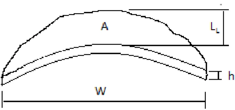
Broken ice pieces can be represented simplistically as rectangular or triangular in shape. In that study, the longest dimension is defined as width W and the
perpendicular dimension as length LL as shown in Figure 1. Most data on piece size
were reported as piece area A, LL, W, LL/W ratio and ice thickness h.
Figure 1. Characterization of a broken ice piece
The scalability of EG/AD/S ice was first examined using piece size data from a variety of simple sloping structures including measurements from three multifaceted cones (Metge and Tucker, 1990; Irani and Timco, 1992; and Lau et al, 1993), three smooth cones (Lau et al, 1988; Lau and Williams, 1991; and Sodhi et al, 1985) and a sloping plane (Timco, 1984). These model tests were performed in standardized
urea ice or EG/AD/S ice, with the exception of Metge and Tucker’s tests which were conducted in thick naturally grown saline ice. Despite slight differences in model shape, these tests were conducted in targeted ice and structure conditions similar to one another.
The problem of predicting ice piece size has generally been considered using the theory of an elastic thin beam (or plate) resting on an elastic foundation (Hetenyi, 1946). In the case of a semi-infinite plate, this theory stipulates that the length of the broken pieces LL is governed by its characteristic length lc as given below
(Cammaert and Muggeridge, 1988):
4 1 2 3 1 12 4 4 w c L v Eh l L (Eq. 1)where E is the elastic modulus of ice, is the Poisson ratio (assumed to be 0.3), and w is the specific weight of water. This lc is related to the thickness of the ice since it
is proportional to h3/4. It is usually measured in the tank as the purely elastic portion of the ice deflection although there are also some primary creep components that affect the loading process. Nevertheless, it is an important index to characterize the flexural deformation of the ice sheet taking account of its flexural rigidity as well as the stiffness of the water foundation.
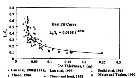
Lau et al (1999) presented the piece size data as the ratio of piece size to characteristic length, LL/lc, as a function of ice thickness for the seven sets of model
test data as shown in Figure 2. The data indicate a clear relationship between the LL/lc and ice thickness despite of a large variation of ice strength.
.
Figure 2. Ratio of ice piece size to characteristic length, LL/lc, versus ice thickness for
seven sets of model test data with sloping structures (Lau et al, 1999) Simple elastic thin plate theory predicts a value of 0.78 for the ratio LL/lc, and the
value is independent of ice thickness (Afanas’ev et al, 1971). However, Figure 2 shows that this is valid only for very thin ice, and the ratio decreases with increasing ice thickness. The dependency of piece size on ice thickness reflects the complexity of the icebreaking process and contributes to the scale effect. Nevertheless, the data also suggest a lower limit of 0.1 for the ratio LL/lc, and beyond a certain thickness
(~9 cm), the non-dimensional piece size approaches that found in full scale. The data suggested that scaling of piece size produced by similar flexural bending
process with model ice thicker than or equal to 9 cm may be considered satisfactory, despite the scale effect inherent in model ice. The tests conducted by Metge and Tucker (1990) and Lau et al (1993) with ice sheets thicker than 9 cm clearly reflect a similar viewpoint.
The failure process of the ice is highly inelastic and there is a large shear component in the ice when thickness increases so this greatly complicates things. Lau et al (1999) offers a hypothesis and preliminary analysis to explain this scale effect by including transverse shear action using thick beam theory. The readers are referred to the paper for details.
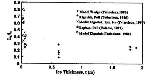
Further review of tests with icebreakers (both model and full scale) confirmed the above finding (Lau et al, 1999). Figure 3 shows the non-dimensional piece size observed in the wake of six icebreaker hulls (both model and full scale) taken from Tatinclaux (1986) with a model wedge and the Kigoriak in both model and full scale trials, and Valanto (1993) with the IB Kapitan Sorokin. This figure indicates a limiting value of 0.2 for LL/lc in thicker ice as shown by the figure. This value is higher than
0.1 associated with the cone tests. It may be due to the different icebreaking processes observed.
We therefore assume a value of 0.1 for conical structures and 0.2 for ships for the dimensionless quantity LL/lc based on Lau et al (1999).
Figure 3. Model/full scale icebreaker test results for varying speeds in urea and sea ice showing the effect of ice thickness on the ratio of ice piece size to characteristic
length, LL/lc. (Lau et al, 1999)
2.2 Re-examined and supplemented model- and full-scale data from CCGS R-Class icebreakers
Newbury (1989) performed preliminary investigation of model ice failure pattern and piece size generated by the CCGS R-Class icebreaker bow form. He analyzed high quality bow prints obtained from scaled R-Class model test performed in EG/AD/S model ice thickness (h) ranging from 1.1 cm to 9.2 cm and compared the results to those reported from both the CCGS icebreakers Kigoriak (h = 0.49 m to 0.74 m) and Pierre Radisson (h = 1 m) sea trials (Anonymous, 1984). In this study, these data were re-examined and supplemented with additional data on the 1:8 scaled R-Class model tests that extends the model test data range to 12.8 cm. It allows further examination of the trends reported by Lau et al (1999) as given in the previous section.
2.2.1 Effect of ship parameters on piece size
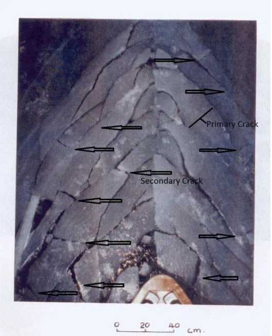
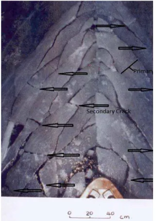
Figure 4 shows the breaking pattern made by the 1:8 R-Class model tested in 9 cm EG/AD/S model ice. This breaking pattern is typical of those made by conventional icebreakers. The size and shape of the broken ice pieces are influenced not only by ice properties, but also by ship parameters such as speed and bow geometry.
Newbury pointed out the importance of ship speed (or ‘velocity of attack’) in determining piece size. For example, the bow angle is smallest near the stem
entrance, which has the largest velocity of attack. This in turn effectively increases the stiffness of the elastic foundation on which the ice rests through increased water pressure and thus creates more cracks in ice and smaller ice pieces at the stem area. The slender ice pieces generated by primary cracking are prone to further breaking (especially along the long sides) due to large or sudden changes of bow curvature along their path and hence with further size decreases. Figure 4 also shows the evidence of increasing secondary breaking when the broken pieces slide along the bow (increased intensity is indicated by increased concentration of
arrows).
Figure 4. Bow print of 1:8 scale R-Class model tested in 0.09 m EG/AD/S model ice. Arrows indicate secondary breaking.
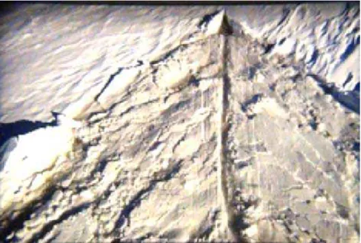
Figure 5 shows a bow print made by the CCGS Sir John Franklin during its 1991 Notre Dame Bay trials (Williams et al, 1992) where the ice thickness was between 0.5 to 0.6 m. Although the crack pattern was obscured by snow cover, we can still discern the general breaking pattern that was similar to that made by the R-Class model (see Figure 4).
Figure 5. Bow print of the CCGS icebreaker Sir John Franklin taken during its 1991 sea trials
2.2.2 Effect of ice thickness on piece size
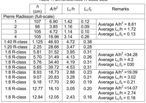
Table 1 summarizes the dimensionless R-Class data. The non-dimensional piece size (non-PS) is parameterized using A/h2, LL/h and LL/lc. In this analysis, the
dimensionless ratio LL/lc is calculated for comparison with Lau et al’s non-PS curve
(see Figure 1). To compare the Pierre Radisson piece size data with the previous datasets in Figure 3, we compute lc and LL using Equation 1 assuming a Young’s
modulus of 4 GPa in the absence of a measure of Young’s modulus, as this value is usually between 3-5 GPa for sea ice with salinity of 5 ppt at -10oC (Gagnon and Jones, 2001). For 1-m sea ice, lc is equal to 13.8 m.
For this dataset, the average values of A/h2, LL/h and LL/lc are equal to 8.61, 1.72
and 0.13, respectively, for the Pierre Radisson sea trials conducted in 1-m sea ice, while these values increase to 14.07, 2.74 and 0.18, respectively, for the 1:8 scaled model tested in 0.128 m (1.02 m full-scale) EG/AD/S model ice. The increases amount to 63%, 59% and 38%, respectively. For the ice-thickness-scaled
parameters, if we compare piece size directly as a function of scaled ice thickness, the simulated piece size is about 60% bigger in terms of both broken piece area A or
length LL. Newbury offered an explanation of the moderately larger than expected
piece sizes observed in model tests by pointing out the cracks visible in the broken model ice pieces that indicate a tendency toward smaller piece sizes in EG/AD/S model ice, which would give a closer agreement with the full scale observation.
Table 1. Dimensionless R-class data h
(cm) A/h
2
LL/h LL/lc Remarks
Pierre Radisson (full-scale)
1 107 6.90 1.42 0.12 Average A/h2 = 8.61 Average LL/h = 1.72 Average LL/lc = 0.13 2 98 3.85 1.16 0.09 3 105 4.72 1.14 0.10 4 105 18.96 3.14 0.26 1:40 R-class 1.125 46.93 4.72 0.38 1:20 R-class 2.25 28.66 3.47 0.28 1:8 R-class 5.81 31.52 3.95 0.31 Average A/h2 =34.28 Average LL/h = 4.2 Average LL/lc = 030 1:8 R-class 5.70 31.49 4.13 0.26 1:8 R-class 5.76 34.40 4.19 0.31 1:8 R-class 5.65 39.72 4.53 0.31
1:8 R-class 8.93 18.73 2.88 0.23 Average A/h2 =19.09
Average LL/h = 3.02
Average LL/lc = 0.21
1:8 R-class 9.07 20.83 3.28 0.21
1:8 R-class 9.18 17.70 2.90 0.19
1:8 R-class 12.77 16.10 3.05 0.20 Average A/h2 =14.07
Average LL/h = 2.74
Average LL/lc = 0.18
1:8 R-class 12.84 12.05 2.43 0.16
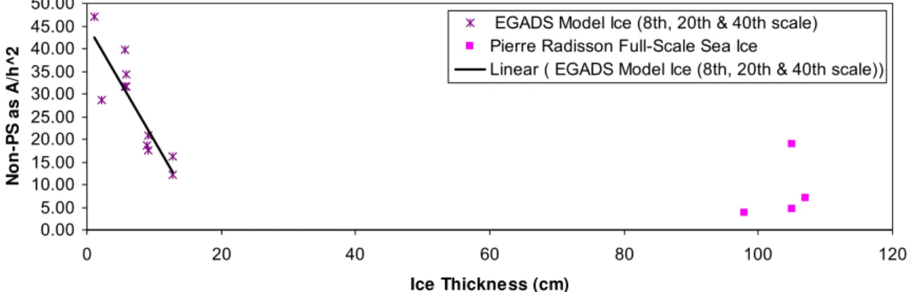
Figures 6, 7 and 8 further show the influence of ice thickness h, on the non-dimensional piece size (non-PS) variable A/h2, LL/h and LL/lc, respectively, for the
same dataset. In Figure 8, the R-Class dataset (highlighted) is compared with the other datasets report earlier by Lau et al (1999). These figures show a strong piece-size dependency on ice thickness in keeping with the trend exhibited by other
0.00 5.00 10.00 15.00 20.00 25.00 30.00 35.00 40.00 45.00 50.00 0 20 40 60 80 100 120 Ice Thickness (cm) N o n -P S as A /h ^ 2
EGADS Model Ice (8th, 20th & 40th scale) Pierre Radisson Full-Scale Sea Ice
Linear ( EGADS Model Ice (8th, 20th & 40th scale))
Figure 6. Non-dimensional piece size defined as A/(h2) as a function of ice thickness
0.00 0.50 1.00 1.50 2.00 2.50 3.00 3.50 4.00 4.50 5.00 0 20 40 60 80 100 120 Ice Thickness (cm) N on-P S a s LL /h
EGADS Model Ice (8th, 20th & 40th scale) Pierre Radisson Full-Scale Sea Ice
Linear ( EGADS Model Ice (8th, 20th & 40th scale))
Figure 7. Non-dimensional piece size defined as LL/h as a function of ice thickness
It should be noted that the 1:8 scale R-Class model test were performed at NRC-OCRE Ice Tank with ice properties similar to that used in the Polar icebreaker tests. We tested the Polar Icebreaker model in EG/AD/S model ice at 8 cm and 10.4 cm, and at this range we expect the similar thickness dependency. However, the bow breaking pattern of the Polar icebreaker model produced larger pieces in
comparison with the R-Class as shown in Figure 9, in which the bow print of the Polar icebreaker model tested in similar ice thickness of 10.4 cm is given. It points to a need for further assessment of the bow shape influence on broken piece size. The bow prints shown in Figure 9 are at the same scale to assist reader’s
comparison.
(a) 1:8 scale R-Class model in 9 cm (b) Polar icebreaker model in 10.4 cm
Figure 9. Comparison of bow prints of two icebreakers in EG/AD/S ice
3 SIZE OF ICE PIECES GENERATED ALONGSIDE ICEBREAKER
The Canadian Coast Guard (CCG) has requested additional analysis of the icebreaking pattern and piece size observed alongside the USCGC icebreaker Polar Star during its 1994-1995 Antarctic Expedition (Keinonen, 1998). This section describes the dataset, analysis procedure and the resulting piece size information.
3.1 Summary of icebreaker USCGC Polar-Star sea trial
In the sea trial of 1994/1995, there were ice measurement activities such as ice thickness, density, salinity and temperature to support the environmental data for
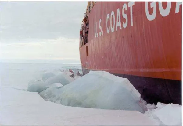
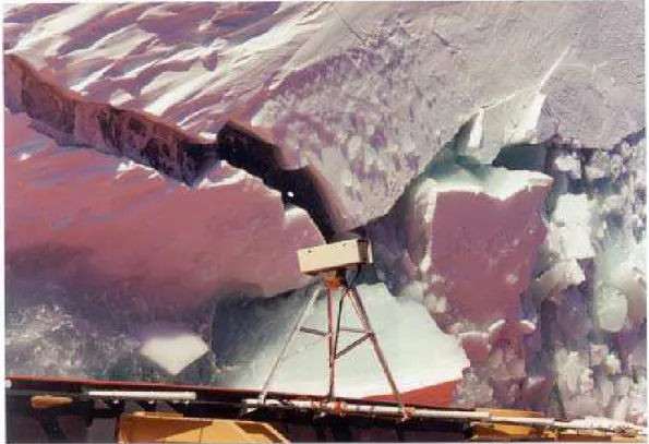
the propeller performance evaluation. Figure 10 shows typical cusps observed during the sea trial. A total of 18 videos (NRC, 1995) were recorded using the side-view camera. Among 100 hours of videos, raw footage was extracted from the first 5 minutes of recording taken from coring site no. 18. Figure 11 shows the location of camera installation on board the vessel. Table 2 shows ice measurement results at the coring site (Newbury and Kirby, 1995).
Figure 11. Camera installation on board the USCGC Polar Star
Table 2. Ice Measurement of Core 032, Site 18: air temperature 0.5◦C, snow depth 0.05 m, ice thickness 2.35 m
Depth (cm) Ice Temp
(◦C) Salinity (ppt) Flexural Strength (kPa) 5 -0.6 1.38 219 15 -1.6 4.62 228 25 -1.9 4.27 294 35 -2.1 4.96 282 45 -2.0 6.19 216 55 -2.1 7.95 174 65 -2.2 5.97 248 75 -2.3 6.49 239 85 -2.4 5.97 271 95 -2.4 5.90 274 105 -2.3 5.97 260 115 -2.4 5.25 304 125 -2.4 4.75 331
3.2 Image analysis procedure
Figure 12 shows the typical view of recorded videos. From GPS information (time and position) annotated in the videos, the ship’s speed and position are estimated and summarized in Table 3.
Figure 12. Typical snap shot captured from the Polar Star Video (red grid is reference scale)
Table 3. Ship Distance and Speed Stitched Image No. Distance (m) Speed (m/s) 1 93.0 1.86 2 66.3 1.33 3 79.3 1.59 4 62.3 1.25 5 86.3 1.73 6 76.9 1.53
From this grid in Figure 12, the scale ratio between image pixels and meters is calculated and applied to compute the size of ice pieces. For convenience, snap-shots in one second intervals were captured from the movie file prior to image processing. The still images were then stitched together to identify the cusps which
were too large to be captured in a single image. Fiji toolkit was used for stitching and processing images. The stitching uses smooth boundary connections and common specific image features like ice cracks. A spline curve was then generated from this image mosaic to estimate the broken cusp size. The final composites are shown in Figure 13.
To extract piece size data, care was taken to identify full cusps that were generated. Due to the lower velocity of attack at the shoulder as explained in Section 2.2.1, the piece size generated at this location is expected to be bigger than those generated from the bow; nevertheless, it provides valuable estimate of piece size to compare with other datasets.
Table 4 summarizes the measured length and width of each cusp taken from each respective photo. The area A of each cusp was estimated by assuming the cusp can be idealized as an arc segment of a circle with height equal to LL and width equal to
W. Table 4 also gives the values of non-dimensional piece sizes, A/h2 and LL/h, for
this dataset. Despites this approximation, the dimensionless variables A/h2 and the
LL/h obtained from the Polar Star at 2.35 m sea ice were 7.33 and 1.59, respectively,
in comparison with their corresponding values of 8.61 and 1.72 for the Pierre Radisson.
For details of the image stitching procedure, please refer to Preibisch et al (2009). Table 4. Cusp dimensions with non-dimensional piece size values of the Polar Star
dataset Image No. Cusp No. W (m) LL (m) A (m2) A/h 2 LL/h 1 1 21.90 3.96 46.34 15.70 1.69 2 1 14.00 2.34 18.89 5.93 1.00 3 1 22.25 3.99 47.82 16.08 1.70 4 1 23.67 4.10 54.06 17.57 1.74 5 1 19.55 4.05 37.12 14.34 1.72 2 25.10 4.37 60.80 19.86 1.86 6 1 13.66 3.34 18.27 8.26 1.42
(1) (2) (3) (4) (5) (6)
4 CORRELATION OF MODEL- AND FULL-SCALE CHANNEL WIDTH DATA
Channel width depends on the icebreaking process. Extensive full-scale ice trials of USCGC Healy (Sodhi et al., 2001) were performed in 2000 shortly after its delivery to the US Coast Guard. The ice thickness was in the range of 0.6 to 1.75 m and the ice flexural strength varied from 190 to 400 kPa. During two trials, the width of the broken channel created by the ship after a series of continuous icebreaking tests was measured to compare with the respective model test; this was used to validate the icebreaking processes simulated at model scale. The width of the channel was measured at a spacing of 1 m for a distance of 67 m on May 4 and 100 m on May 6 by stretching a rope across the channel. Figure 14 shows plots of channel width reported by Tucker (2001). The average ice thicknesses on these two days were, respectively, 1.35 and 1.73 m, and the channel widths Wc were 32.28 and 31.36 m.
The gap Gc between the sides of the ship to the edge of intact ice is half the
difference between the average channel width and the maximum ship’s beam (25 m). The ratio of gap to ice thickness (Gc/h) was 2.77 for 1.35 m thick ice sheets
and 1.83 for 1.73 m thick ice sheets.
Figure 14. Channel width created by the Healy on a straight run during sea trials (Tucker, 2001)
Following the full-scale trials, a complete set of resistance, propulsion, and manoeuvring model tests with a 1:23.7 scale model of the ship were performed in
scaled ice conditions at the NRC-OCRE Ice Tank for correlation with the full-scale data (Jones and Moores, 2002 and Lau, 2006). Broken channel width was measured at 2-m intervals after tests in three level ice sheets and these are summarized in Table 5. For 0.031-m (0.73 m scale), 0.0424-m (1.00 m full-scale) and 0.0418-m (0.99 m full full-scale) ice sheets, the ratio of gap to ice thickness was 2.56, 2.02 and 2.56, respectively, which are within the range of the full scale values, i.e., 1.83 to 2.77.
Table 5. Summary of channel width created by the Healy model Test # of data points h (m) Wc (m) Gc (m) Gc/h Healy_16 12 0.031 1.21 0.080 2.56 Healy_17 8 0.042 1.22 0.086 2.02 Healy_18 22 0.041 1.26 0.107 2.56
The channel width data for the Polar icebreaker model tests were also analyzed in the same way as the Healy model tests for the straight ahead runs B3_126, B3_128 and B4_133, in which channel measurements were performed at 2-m intervals along the broken ship track and the ratio of gap to ice thickness Go/h ranged from 1.10 to
1.45. The result is summarized in Table 6.
Table 6. Summary of channel width created by the Polar icebreaker model Test # of data points h (m) Wc (m) Gc (m) Gc/h B3_126 17 0.100 1.40 0.142 1.42 B3_128 12 0.100 1.34 0.110 1.10 B4_133 12 0.090 1.38 0.131 1.45
The channel width created by the model of Healy compared well with those measured during its ice trials with the ratio of gap to ice thickness within the range of full-scale data. This gives additional support to the validity of simulated icebreaking processes during model tests. On the other hand, the Polar icebreaker gives a smaller gap to thickness ratio ranging from 1.1 to 1.45. This difference in channel width may suggest a large influence of the hull geometry on the icebreaking process.
5 CONCLUSIONS
Icebreaking is a complex process: the size and shape of the resulting ice pieces are influenced not only by ice properties but also by ship parameters such as speed and bow geometry. This study is focused on ice properties, in particular the correlation of model-scale EG/AD/S ice to full-scale sea ice; the effect of ship parameters on piece size was not examined. A review of the model-scale/full-scale correlation study on data with five icebreakers (Lau and Wang, 2012) has shown a good agreement
between NRC-OCRE performance predictions from model test data and full-scale measurements in resistance, power and manoeuvring. To add to this work, we have examined the scalability of EG/AD/S model ice regarding broken piece sizes,
focusing on limited datasets collected from conventional icebreakers operating in the Canadian Arctic.
This study has shown the non-dimensional piece size decreases and approaches that found in full scale beyond a certain thickness: in particular, the scaling of piece size with model EG/AD/S ice equal to or thicker than 9 cm thick may be considered satisfactory despite the scale effect inherent in model ice.
Analysis of R-Class and Polar Star data further substantiates the aforementioned trend. In the case of R-Class model tests that were conducted at a thickness range used in the Polar icebreaker model test program, the simulated piece size scales to about 60% bigger at full scale. Evidence of secondary cracking captured on bow prints of model tests also indicates a tendency toward smaller piece sizes in EG/AD/S model ice, which would give a closer agreement with the full scale
observation. We expect the EG/AD/S ice would scale piece size within this level of accuracy.
We tested the Polar Icebreaker model in EG/AD/S model ice at 8 cm and 10.4 cm, and at this range we expect similar thickness dependency. However, the bow breaking pattern of the Polar icebreaker model produced much larger pieces in comparison with the R-Class tested in similar ice thickness. It points to a need for further assessment of the influence of bow shape on broken piece size, as the Polar icebreaker designs have bow geometry which significantly diverge from the
traditional icebreaker bow forms that may contribute to different icebreaking patterns and hence piece size.
6 REFERENCES
Afanas’ev, V.P., Dolgopolov, Y.V., and Shvaishstein, Z.I., 1971. Ice pressure on individual marine structures, in Studies in Ice Physics and Ice Engineering, Edited by G.N. Yakovlev, Published by Israel Program for Scientific Translations, Jerusalem, Israel, pp. 50-68.
Anonymous,1984. Modelling the broken channel, final report prepared for the Canadian Coast Guard by Arctec Canada Limited and Dome Petroleum Limited, Transportation Development Centre Report TP5373E, Montreal.
Cammaert, A.B. and Muggeridge, D.B., 1988. Ice Interaction with Offshore Structures, Published by Van Nostrand Reinhold, New York.
Gagnon, R. and Jones, S.J., 2001. Elastic properties of ice, Chapter 9 of Handbook of Elastic Properties of Solids, Liquids and Gases, ed. Levy, Bass and Stern, Vol. III: Elastic Properties of Solids: Biological and Organic Materials, Earth and Marine Sciences: 229-257.
Hetenyi, M., 1946. Beam on Elastic Foundations, University of Michigan Studies, Scientific Series, Vol. XVI, The University of Michigan Press.
Howard, D. and Abdelnour, R., 1987. The testing of the 1:8 scale model of the R-class in level ice, Transportation Development Centre Report TP8828E, Submitted by ARCTEC Newfoundland Limited, Transportation Development Centre, Quebec. Irani, M.B. and Timco, G.W., 1993. Ice loading on a multifaceted conical structure, Proc. 3rd International Offshore and Polar Engineering Conf., Singapore, Vol. 2, pp. 520-558.
Jones, S.J. and Moores, C., 2002. Resistance tests in ice with the USCGC Healy, IAHR 16th International Symposium on Ice, Dunedin, New Zealand, Vol. 1, p. 410-415.
Keinonen, A., Browne, R.P., Edgecombe, M.H. and Revill, C.R., Ritch, R., 1998. USCGC Polar Star propeller ice load measurements, 1994-1995 : trials, analysis and results Vol. 1, Transportation Development Centre Report no. TP13268E, Transport Canada.
Lau, M., 1999. An analysis of icebreaking pattern and ice piece size around sloping structures, 18th International Conference on Offshore Mechanics and Arctic Engineering - OMAE99, Paper OMAE-1151, St. John’s, Newfoundland, Canada. Lau, M. and Wang, J.Y., 2012. A brief summary of model-scale/full-scale correlation of OCRE’s model test results in supporting the CCG Polar Icebreaker model test data evaluation, OCRE-TR-2012-28, National Research Council Canada
Lau, M., Wang, J.Y. and Lee, C.J., 2007. Review of ice methodology, Proc. 14th
International Conference on Port and Ocean Engineering under Arctic Conditions, Dalian, China, pp. 350-362.
Lau, M., Jones, S.J., Tucker, J.R., and Muggeridge, D.B., 1993. Model ice ridge
forces on a multi-faceted cone, Proc. 12th International Conference on Port and
Ocean Engineering under Arctic Conditions, Vol. 2, Hamburg, pp. 537-546.
Lau, M., Muggeridge, D.B., and Williams, F.M., 1988. Model tests of fixed and free
floating downward breaking cones in ice, Proc. 7th International Conference on
Offshore Mechanics and Arctic Engineering, Houston, pp. 239-247.
Lau, M. and Williams, F.M., 1991. Model ice forces on a downward breaking cone, Proc. 11th International Conference on Port and Ocean Engineering under Arctic Conditions, Vol. 1, St. John’s, pp. 167-184.
Maattanen, M., 1986. Ice sheet failure against an inclined wall, Proc. 8th IAHR Ice Symposium, Vol. 1, Iowa City, pp. 149-158.
Metge, M. and Tucker, J.R., 1990. Multifaceted cone tests -- Year two, 1989-1990, Technical Report, Esso Resources Canada Limited, Calgary, Alberta.
Newbury, S. 1989. A preliminary investigation of model ice failure pattern and piece
size generated by an icebreaker bow form, Proceeding of 22nd American Towing
Tank Conference, 8-11 August 1989, St. John's, Newfoundland.
Newbury, S. and Kirby, C., 1995. Ice measurements in support of propeller load evaluation on the USCGC Polar Star in the Antarctic summer environment 1995, TR-1995-15, National Research Council Canada.
NRC, 1995. Video of the USCGC Polar Star Antarctic trials during December 1994/January 1995, Archived footage, National Research Council Canada.
Preibisch, S., Saalfeld, S. and Tomancak P., 2009. Globally optimal stitching of tiled 3D microscopic image acquisitions, Bioinformatics, 25(11): 1463-1465.
Sodhi, D.S., Griggs, D.B. and Tucker, W.B., 2001. Healy ice trials: Performance
tests in ice, Proc. 16th International Conference on Port and Ocean Engineering
under Arctic Conditions, Vol. 2, pp.893-907,
Sodhi, D.S., Morris, C.E. and Cox, G.F., 1985. Sheet ice forces on a conical
structure - An experimental study, Proc. 9th International Conference on Port and
Ocean Engineering under Arctic Conditions, Vol. 2, Narssarssuaq, pp. 643-655. Tatinclaux, J.C., 1986. Ice floe distribution in the wake of a simple wedge, Proc. 5th International Conference on Offshore Mechanics and Arctic Engineering, Vol. 4, Tokyo, pp. 622-629.
Tucker, T., 2001. Ice conditions and properties during the Healy ice trials, US Army ERDC-CRREL, in USCGC Healy Ice Trials 2000 Consolidated Report USCG-ELC-023-01-09, October 2003 and Associated Reports CD.
Timco, G.W., 1992. Second report of the IAHR working group on ice-modelling
materials, Proc. 11th IAHR Symp. on Ice Problems, Banff, Canada.
Timco, G.W., 1986. EG/AD/S: A new type of model ice for refrigerated towing tanks, Cold Regions Science and Technology, 12: 175-195.
Timco, G.W., 1984. Model Tests of ice forces on a wide inclined structure, Proc. 7th IAHR Ice Symposium, Vol. 2, Hamburg, pp. 89-96.
Valanto, P., 1993. Investigation of icebreaking pattern at the bow of the IB Kapitan
Sorokin on the Yenisei River Estuary in May 1991, Proc. 12th International
Conference on Offshore Mechanics and Arctic Engineering, Vol. 4, pp. 127- 134. Williams, F.M. et al, 1992. Full scale trials in level ice with Canadian R-Class