Publisher’s version / Version de l'éditeur:
Vous avez des questions? Nous pouvons vous aider. Pour communiquer directement avec un auteur, consultez la première page de la revue dans laquelle son article a été publié afin de trouver ses coordonnées. Si vous n’arrivez pas à les repérer, communiquez avec nous à [email protected].
Questions? Contact the NRC Publications Archive team at
[email protected]. If you wish to email the authors directly, please see the first page of the publication for their contact information.
https://publications-cnrc.canada.ca/fra/droits
L’accès à ce site Web et l’utilisation de son contenu sont assujettis aux conditions présentées dans le site LISEZ CES CONDITIONS ATTENTIVEMENT AVANT D’UTILISER CE SITE WEB.
6th Transportation Specialty Conference [Proceedings], pp. 188-1-188-10,
2005-05-01
READ THESE TERMS AND CONDITIONS CAREFULLY BEFORE USING THIS WEBSITE. https://nrc-publications.canada.ca/eng/copyright
NRC Publications Archive Record / Notice des Archives des publications du CNRC : https://nrc-publications.canada.ca/eng/view/object/?id=22883f39-5070-45af-a9c5-7cc1f126ba44 https://publications-cnrc.canada.ca/fra/voir/objet/?id=22883f39-5070-45af-a9c5-7cc1f126ba44
NRC Publications Archive
Archives des publications du CNRC
This publication could be one of several versions: author’s original, accepted manuscript or the publisher’s version. / La version de cette publication peut être l’une des suivantes : la version prépublication de l’auteur, la version acceptée du manuscrit ou la version de l’éditeur.
Access and use of this website and the material on it are subject to the Terms and Conditions set forth at
Effectiveness of predictive models for estimating asphalt concrete
complex modulus
http://irc.nrc-cnrc.gc.ca
N a t i o n a l R e s e a r c h C o u n c i l C a n a d a
Effe c t ive ne ss of pre dic t ive
m ode ls for e st im at ing a spha lt
c onc re t e c om plex m odulus
N R C C - 4 7 6 8 3
Z e g h a l , M . ; A d a m , Y . E . ;
E l H u s s e i n H . M o h a m e d
A version of this document is published in / Une version de ce
document se trouve dans:
6
thTransportation Specialty Conference, Toronto, Ontario,
June 2-4, 2005, pp. 1-10
6th Transportation Specialty Conference 6e Conférence spécialisée sur le génie des transports
Toronto, Ontario, Canada
June 2-4, 2005 / 2-4 juin 2005
EFFECTIVENESS OF PREDICTIVE MODELS FOR ESTIMATING
ASPHALT CONCRETE COMPLEX MODULUS
M. Zeghal1, Y.E. Adam2 and H.H. Mohamed1
1. National Research Council Canada, Institute for Research in Construction, Ottawa, ON, Canada 2. Carleton University, Ottawa, ON, Canada
ABSTRACT: The complex modulus has been identified as a suitable mechanistic characterisation
technique for asphalt concrete because of its ability to capture the visco-elastic response of the material and has since been incorporated in the new AASHTO 2002 road design guide. The pavement research group of NRC developed a laboratory testing protocol involving a wide range of loading frequencies and temperature conditions to satisfy requirements of a variety of analytical models. The high cost of the test motivated developers of the ASSHTO guide to implement predictive models as an alternative to actual laboratory test results in lower design levels. This paper discusses results of the tests performed at NRC on typical asphalt concrete mixes and calls for establishing a material library for Canadian users of the ASSHTO guide. The predictive equation came short of accurately estimating laboratory measured dynamic modulus. The generic material properties listed in the library could be used instead of the ASSHTO predictive equation.
1. INTRODUCTION
Gaps in the knowledge base delayed the development of effective analytical models for road design and analysis using sound principles of mechanics and dictated reliance on empirical procedures. These empirical design procedures were based on some indices, and at best, on physical properties to characterize the different materials used in building roads. This approach was applied to asphalt concrete where attempts are made to use the mix design process to produce a material with adequate resistance to known forms of damage, mainly rutting. The process is done completely in isolation from the structural design process, which is supposed to consider the characteristic response of the material. Attempts to overcome limitations of the current practice led to the development of the AASHTO 2002 new design guide where the asphalt concrete materials are mechanistically characterised using the complex modulus concept. The complexity and time consuming nature of the laboratory test adopted in the advanced design (level 1) motivated developers of the AASHTO 2002 design guide to introduce two more basic designs (level 2 and 3) which do not require mechanistic material data and hence, no testing to characterise asphalt concrete materials. More precisely, level 2 and 3 were designed to rely on predictive equations to evaluate the complex modulus of asphalt concrete materials. Due to the limited capabilities of current asphalt concrete (AC) testing systems available in Canada, it is expected that level 3 design will be relied upon by practitioners. Hence the effectiveness of the predictive model incorporated in AASHTO 2002 guide to estimate the complex modulus was evaluated in this paper. The evaluation process relied on comparison between model predictions and laboratory measurements of dynamic modulus of asphalt concrete materials.
2. THE COMPLEX MODULUS 2.1. Concept
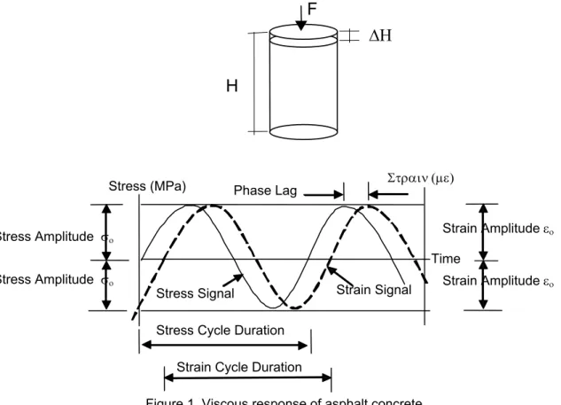
Characterisation of asphalt materials focussed on capturing the known viscoelastic behaviour of the material. Within this viscoelastic domain, the response of an asphalt concrete material to sinusoidal loading is also sinusoidal but with a phase lag (Sayegh 1967) as shown in Figure 1.
F
ΔΗ
H
Stress Amplitude σο
Stress Signal Strain Signal Stress (MPa)
Stress Cycle Duration
Στραιν (με)
Strain Cycle Duration Phase Lag
Time Stress Amplitude σο
Strain Amplitude εο
Strain Amplitude εο
Figure 1. Viscous response of asphalt concrete
Simulating traffic loading in the laboratory involves subjecting asphalt concrete to sinusoidal loadings at different frequencies within the linear viscoelastic range. Loading could be performed under either a stress- or strain-controlled mode. In the first case, a specific stress value is applied and the corresponding strain is obtained, while in the other case, specific strain amplitude is applied and the corresponding stress is recorded. Equations 1 to 5 describe the viscoelastic approach mathematically (Heck et al. 1998, Richard et al. 2003, Ferry 1980 and Sayegh 1967)
In the stress-controlled case the stress applied is given by: [1] σ = σ0Sin (ω.t)
And the corresponding strain is given by: [2] ε = ε0Sin (ω.t-φ)
In the strain-controlled case the applied strain is expressed as: [3] ε = ε0Sin (ω.t
And the corresponding stress is given by: [4] σ = σ0Sin (ω.t+φ)
where σ0 is the stress amplitude, ε0 is the strain amplitude (see Figure 1) and ω is the angular velocity
related to the frequency f by Equation 5: [5] ω = 2πf 3.5
φ is the phase angle related to the time that the strain lags the stress (see Figure 1). The phase angle is an indicator of the degree of the viscoelastic behaviour of asphalt concrete mix. The phase angle φ values are limited to between 0 and π/2. A value of 0 is an indicator of a purely elastic behaviour, while a value of π/2 is an indicator of a purely viscous behaviour
It is useful to express the sinusoidal relations in the complex notation in which they are commonly dealt with. Hence, the previous functions can be rewritten as follows:
In the stress-controlled case the applied stress function is given by Equation 6: [6]
σ σ
=
0.
e
iwtThe corresponding strain is given by Equation 7: [7]
ε ε
=
0.
e
i wt( −φ)In the strain-controlled case, the function of the applied strain is expressed as: [8]
ε ε
=
0.
e
i wt( )And the corresponding stress is given by [9]
σ σ
=
0.
e
i wt( +φ)There is general agreement among researchers about the effectiveness of the complex modulus concept in evaluating the fundamental stress-strain response of asphalt concrete mixes. The modulus is a complex number, which defines the relationship between the stress and strain for a linear viscoelastic material subjected to sinusoidal loading. The real part of the complex modulus is a measure of the material elasticity and the imaginary part is a measure of the viscosity. The complex modulus is defined (by analogy to the Young modulus of elasticity) as shown in Equation 10 (Witczak and Root 1974):
[10] 0 1 2 0
* (
)
iE
iw
σ σ
e
φE
iE
ε
ε
=
=
=
+
The ratio of the stress to strain amplitudes defines the absolute value of the complex modulus which is known as the dynamic modulus and is expressed by Equation 11:
[11] * 0
0
E
σ
ε
=
2.2. Laboratory testing technique
The complex modulus test is included in the AASHTO 2002 guide as a mean for characterising asphalt concrete materials and results are used as input for the advanced design (level 1). To determine the dynamic modulus in the laboratory, a test protocol was developed which involved examining the impact of temperature and loading conditions.
The sensitivity of AC materials to temperature requires controlling the temperature of the sample during the test. In this study, five temperatures were used in the test including -10, 0, 20, 30 and 40oC.
Loading was controlled by maintaining a displacement magnitude that produces a response within the linear viscoelastic range of the material. Further, simulation of traffic characteristics dictates controlling the loading frequency to account for different traffic speeds. Six frequencies (0.1, 0.3, 1, 5, 10 and 20 Hz) were used in this study.
A test setup was established to facilitate the necessary control over the above parameters and to collect the data necessary for capturing all components of the material response. The data acquisition system was designed to record the test history involving critical sampling rates capable of recording changes in the stress and strain condition. Laboratory test results, determined at the five temperatures and six frequencies, were used to gauge the effectiveness of the AASHTO 2002 predictive equations in estimating the dynamic modulus of the mix under investigation.
3. PREDICTIVE EQUATIONS
The best approach for obtaining the dynamic modulus of AC materials remains performing a complex modulus test in the laboratory. However, given the complexity and time-consuming nature of the laboratory test procedure, many predictive equations have been proposed to evaluate the dynamic modulus of asphalt mixes using the results of simple and commonly performed aggregate, binder and mix tests. In 1996, Fonseca and Witczak summarized the most important predictive equations developed since 1967 as they are reproduced here in Table 1 (Fonseca and Witczak 1996).
The models presented in Table 1 have several limitations. The major drawback of these equations is associated with the use of classical statistical principles to extrapolate parameters outside the range of the tests performed. The majority of test results were generated within a temperature range of 5 to 40oC. This resulted in unrealistically large and small predictive moduli for very cold and very hot conditions outside this range. Fonseca and Witczak observed that the majority of these predictive equations were based on the original bitumen properties, with the test temperature being the most important variable in the system. However, these predictive equations do not account for the hardening effects on binders, and consequently the AC properties associated with long-term aging.
In 1996, Fonseca and Witczak proposed a predictive equation for the dynamic modulus based on a reasonably large database. Improvements made to earlier models included taking into account hardening effects from short and long-term aging, as well as extreme temperature conditions. Based on the gradation of aggregates in the mix and asphalt binder properties, Witczak proposed the following dynamic modulus predictive model which is currently incorporated in the AASHTO design guide (Fonseca and Witczak 1996). [12] * 2 200 200 4 2 4 38 38 ( 0.603313 0.313351log 0.393532 log )
log
1.249937
0.029232
0.001767(
)
0.002841
0.058097
[3.871977
0.0021
0.00395
0.000017(
)
0.00547
]
0.802208
(
)
1
a beff f beff aE
P
P
P
V
P
P
P
V
V
e
− − − η= −
+
−
+
−
−
+
−
+
−
+
+
+
34V
P
where: *E
= Asphalt mix dynamic modulus, in 105 psi, η = Bitumen viscosity, in 106poise,
f = Loading frequency, in Hz,
Va= Percent air voids in the mix, by volume,
Vbeff = Percent effective bitumen content, by volume,
P34 = Percent retained on ¾-inch sieve, by total aggregate weight (cumulative),
P38 = Percent retained on 3/8-inch sieve, by total aggregate weight (cumulative),
P4 = Percent retained on No. 4 sieve, by total aggregate weight (cumulative), and
Table 1. Summary of dynamic modulus predictive equations
Equation
Number Equation model form
1 6 * 10 0 1 200 2 3 70:10 4
log
E
=
a
+
a p
+
a V
a+
a
η
+
a p
aca5
t
pa6
2log
10E
*= +
b
0b p
1 200+
b V
2 a+
b p
3 acb4(log
η
t) 5
b 3 * ( 2) 10 0 1log
E
=
c
*
c p
−tc 4 2 6 6 7 8 6 7 8 10 12 * 10 0 1 200 3 1 70:10 ( log ) ( log ) 5 9log
(
)
[
]
[
]
d a d d f d d d f d d d p ac p acE
d
d p
f
d V
d
d t
p
d t
p
f
d f
η
+ +=
+
+
+
+
+
+
11 5 4 5 6 * 10 0 1 2 70:10 3log
E
= +
e
e V
a+
e
η
+
e t V
pe beffe 6 6 2 6 8 9 11 8 9 13 * 10 0 1 200 3 4 70:10 5 ( log ) ( log ) 7 10log
(
)
][
12]
g g a g g f g g g f g p p ac optE
g
g p
f
g V
g
g f
g t
g f
t
p
p
g
η
+ +=
+
+
+
+
+
+
−
+
7 6 9 * 10 0 1 2 3 / 4 3 70:10 4 5 2 2 6 7 8 10 4 11 200log
log
(log
*
)
(
)
(
)
(
)
a p hp beff beffopt p beff abs
E
h
h V
h p
h
h t
h
f
h
f
t
h V
V
h
t
h V
p
h
p
p
η
=
+
+
+
+
+
+
+
−
+
+
+
8 6 * 2 2 10 0 1 2 3 200 4 4 5 6 7 8 9 2 2 2 2 2 2 10 200 11 3 / 4 12 3 / 8 13 4 14 15 70:10 16 17 3 / 8 18 3 / 8 19 3 / 4 4 20 3 / 8 4 21 3 / 8log
beff a abs p p beffabs beff beff abs
E
k
k V
k V
k p
k p
k p
k t
k f
k t
k V
k p
k p
k p
k p
k p
k
k f
k p V
k p V
k p
p
k p
p
k p
p
η
=
+
+
+
+
+
+
+
+
+
+
+
+
+
+
+
+
+
+
+
+
+
9 6 * 2 10 0 1 2 3 200 4 5 6 7 2 2 2 2 2 2 8 9 200 10 3 / 4 11 3 / 8 12 13 70:10 14 15 3 / 8 16 3 / 4 17 3 / 4 4 18 3 / 8 4 19 3 / 8log
(
)
beff a abs p p beff absbeff beff abs
E
l
l V
l V
l p
l p
l t
l f
l t
l V
l p
l p
l p
l p
l
l
f
l p
V
l p
V
l p
p
l p
p
l p
p
η
=
+
+
+
+
+
+
+
+
+
+
+
+
+
+
+
+
+
+
2+
10 6 9 * 10 0 1 2 3 70:10 4 5 2 2 6 7 8 10 4 11 200log
(
)
log
log( *
)
(
)
(
)
(
)
beff a p mp beff beffopt p beff abs
E
m
m V
m V
m
m t
m
f
m
f
t
m V
V
m
t
m V
p
m
p
p
η
=
+
+
+
+
+
+
+
−
+
+
+
In the equations shown in Table 1, the alphabetic letters subscripted with numbers are regression coefficients. The other variables have the following definitions and units:
6
70:10
η
= AC viscosity at 70oF (21.1oC), in 106 poiset
η
= AC viscosity at test temperature (t), in poisep
t
= Test temperature, in oFf
= Test frequency of load wave, in Hza
V
= Percent volume of air voids in the mixbeff
V
= Effective asphalt content of mix, by volume percentagebeffopt
V
= Effective optimum asphalt content of mix, by volume percentageabs
p
= Percentage asphalt absorptionac
p
= Percentage asphalt content, by weight of mixopt
3 / 4
p
= Percent weight (by total aggregate weight) retained on 3/4 inch sieve3 / 8
p
= Percent weight (by total aggregate weight) retained on 3/8 inch sieve4
p
= Percent weight (by total aggregate weight) retained on a No. 4 sieve200
p
= Percent weight (by total aggregate weight) passing through a No. 200 sieve4. EVALUATION OF THE PREDICTIVE EQUATION
Different binders, aggregates and mix designs were included in this study. Ministry of Transportation of Ontario (MTO) (1990) specifications were followed in determining the appropriate combinations of different aggregate fractions to achieve the job mix formulae that satisfied gradation requirements outlined for each specific HMA mix type. AASHTO specifications were followed to create job mix formulae that satisfied the gradation curves of SuperPave mix designs (AASHTO 1993). Test specimens were prepared using a hot mix asphalt (HMA 3) typically used as a surface course in Ontario and locally known as HL3. Evaluation of the predictive equation focused on the impact of the binder type only. Specimens from the HMA 3 mix were prepared using a binder content of 5±0.5% (selected using the Marshal mix design procedure). Dynamic modulus predictions produced for different test temperatures and loading frequencies using equation 12 were compared with results from mechanical tests performed according to the test protocol discussed above. Predicted and measured dynamic modulus values for three different temperature conditions (-10, 20 and 40oC) were compared. These temperatures were chosen to represent cold, moderate and warm service temperatures. The selected loading frequencies (0.1, 1 and 20 Hz) represent slow, medium and relatively fast vehicle speeds.
4.1. Physical properties
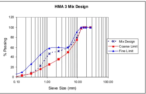
The gradation curve of HMA 3 is illustrated in Figure 2. The gradation fits well within the limits set by MTO for this mix type. Physical characteristics of this mixture are shown in Table 2.
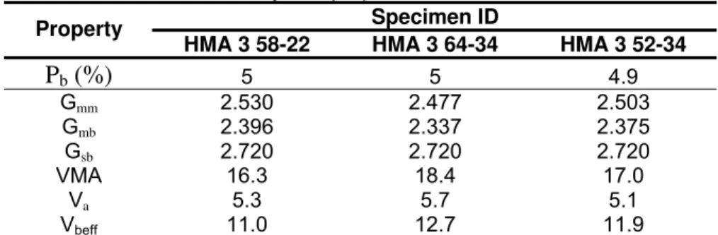
Table 2. Physical properties of HMA 3 mix
Specimen ID Property
HMA 3 58-22 HMA 3 64-34 HMA 3 52-34
P
b(%)
5 5 4.9 Gmm 2.530 2.477 2.503 Gmb 2.396 2.337 2.375 Gsb 2.720 2.720 2.720 VMA 16.3 18.4 17.0 Va 5.3 5.7 5.1 Vbeff 11.0 12.7 11.9 Where• (Pb): Binder content by total mass of mixture
• (Gmm): Maximum specific gravity of mixture
• (Gmb): Bulk specific gravity of compacted mixture
• (VMA): Voids in mineral aggregate as a percent of bulk volume • (Va): Air voids in compacted mixture as a percent of total volume
Figure 2. Gradation curve of HMA 3
4.2. Predicted vs. measured dynamic modulus
he absence of a wide range viscosity-temperature relationship was one of the main obstacles to the
ssessment of the accuracy of predictions performed on HMA 3 mixes prepared with two different binders
tatistical analysis, performed on the data pertaining to the two mixes presented in Table 3 confirmed that
Table 3. Statistical analysis results
Mean Abs ge Percent Error (%)
HMA 3 Mix Design
0 20 40 60 80 100 120 0. 10 1.00 10.00 100.00 Sieve Size (mm) % P a s si n g Mix Design Coarse Limit Fine L imit T
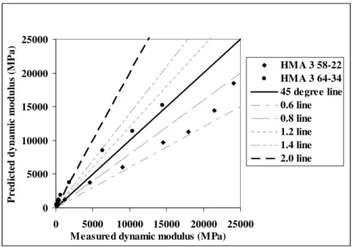
development of accurate predictive equations. This relationship is critical for accurately assessing the rheological behaviour of binders acting as part of the AC mix. In this study, the ability of the predictive equation to discriminate between different binder types was evaluated. A comparison between the predicted values and those determined using the complex modulus testing technique was conducted using the equality line drawn at 45o (see Figure 3). Points located above this line indicate that model predictions over-estimated the dynamic modulus value. Points below the equality line indicate under-estimated values. Actual coordinates of data points (measured and predicted) were used in this study to quantify deviation of predicted values from those measured in the laboratory. Lines that represent different percentages of deviations were used on both sides of the equality line to highlight deviation determined under different conditions. For example, a point falling between the equality line and the 0.8 Line represents less than 20% deviation in the form of under-estimation.
A
(PG 64-34 and PG 58-22) is given in Figure 3. The HMA 3 64-34 results indicate a trend towards over-prediction compared with the measured values, with a deviation of more than 200% within the low modulus state. In contrast, estimates of the HMA 3 PG 58-22 modulus values were mainly under-predicted (with a deviation of up to about 40%), except in the case of small modulus values for which over-predictions of less than 20% were observed.
S
the predictive equation possesses limited capabilities for predicting the dynamic modulus of mixes with engineered binders as reflected in the high average percent errors (169%). Predictions of the response for the mix with a conventional binders (PG 58-22) using equation 12, were better as indicated by lower average percent errors given in Table 3.
olute error (MPa) Avera Equation
HMA 3 64-34 HMA 3 58-22 HMA 3 64-34 HMA 3 58-22
0 5000 10000 15000 20000 25000 0 5000 10000 15000 20000 25000 Measured dynamic modulus (MPa)
Pr ed ic te d dy na m ic m o dul us ( M P a ) 1 HMA 3 58-22 HMA 3 64-34 45 degree line 0.6 line 0.8 line 1.2 line 1.4 line 2.0 line
Figure 3. Evaluation of predictions made for HMA 3 mix with different binder grades
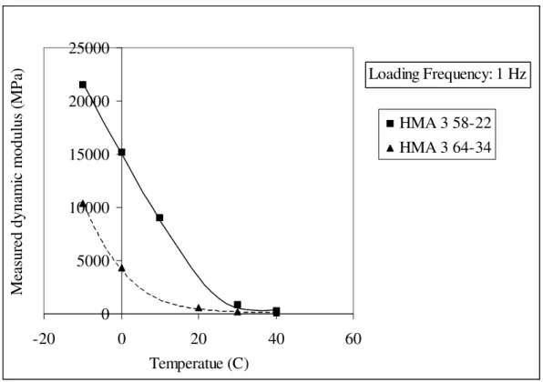
The impact of the binder grade on the mix response was further analyzed. The dynamic modulus values at different temperatures are shown in Figure 4 and 5 for the predictive equation and the laboratory test results, respectively. The results shown in these two figures indicate that the predictive equation managed to correctly rate the response at low temperatures associated with the two binders. However, the predictive equation under-estimated the difference between the two binders as quantified in the test results. The predictive equation showed a difference of only 27% compared with the measured response, which reflects a 100% difference.
0 4000 8000 12000 16000 -20 0 20 40 60 Temperature (C) P redi ct ed dynam ic m odul us ( M Pa) HMA 3 58-22 HMA 3 64-34 Loading Frequency: 1 Hz
0
5000
10000
15000
20000
25000
-20
0
20
40
60
Temperatue (C)
M
eas
ur
ed dyna
m
ic
m
odul
us
(
M
P
a)
HMA 3 58-22
HMA 3 64-34
Loading Frequency: 1 Hz
Figure 5. Measured dynamic modulus vs. temperature
It is clear from the test results that the engineered binder (PG 64-34) will fulfill its purpose, which aims for flexibility by reducing brittleness at low temperatures, hence reducing the potential for cracking. The measured dynamic modulus of the HMA 3 with PG 64-34 is half the value of the HMA 3 with PG 58-22 binder (see Figure 5). Both measured and predicted dynamic moduli of the two binders are identical at high temperatures, reinforcing the role-played by the aggregate skeleton at high temperatures.
5. CONCLUSION
The complex modulus concept is considered as a step forward towards mechanistic characterisation of asphalt concrete materials. In times of shrinking resources for Canadian jurisdictions, circumventing the need for a laboratory complex modulus test using predictive equations is considered a viable alternative. However, the predictive model incorporated in the AASHTO 2002 guide came up short of accurately estimating the dynamic moduli. The average percent errors of dynamic modulus estimation were found to be high for neat binders and unrealistically high for engineered binders. Although the predictive equation failed to quantify the dynamic modulus as measured in the laboratory, it successfully discriminated between the two uniquely different binder grades by rating them correctly with respect to each other. The predictive equation requires further development for effective estimation of the complex modulus and accurate performance determination of roads.
6. REFERENCES
AASHTO 1993. Standard Specifications for SuperPave Volumetric Mix Design. Designation MP2-02. Ferry, J.D. 1980. Visco-elastic properties of polymers. 3rd ed. Wiley, N.Y., USA.
Fonseca, O.A. and Witczak, M.W. 1996. A Prediction Methodology for the Dynamic Modulus of In Place Aged Asphalt Mixture. Journal of the Association of Asphalt Paving Technologist, Vol. 65, pp. 532-565.
Heck, J.V., Piau, J.M., Gramsammer, J.C., Kerzreho, J.P. and Odeon, H. 1998. Thermo- Visco- Elastic Modelling of Pavements Behaviour and comparison with Experimental Data from LCPC Test Track. 5th International Conference on the Bearing capacity of Roads and Airfields. Norway.
Ontario Ministry of Transportation (MTO). 1990. Ontario Provincial Standard Specification, OPSS 1149
-1152, Ottawa, Ontario, Canada
Richard, Y., Youngguk, K., King, M. and Momen, M. 2003. Dynamic Modulus Testing of Asphalt concrete in Indirect tension Mode. Submitted for presentation at the 2004 TRB Annual Meeting, Washington D.
C., USA.
Sayegh, G. 1967. Viscoelastic properties of bituminous mixtures. Proceedings of the 2nd International conference on structural design of asphalt pavement, pp. 743-755. Held at Rackham Lecture Hall,
University of Michigan, Ann Arbor, USA.
Witczak M.W., and Root, R.E. 1974. Summary of Complex Modulus Laboratory Test Procedures and Results. American Society for Testing and Materials, ASTM Special Technical Publication, Vol. 561, pp.