Design and Analysis of Thermal and Structural Systems Through Implementation of Open-Source Finite Element Software

(1)

Design and Analysis of Thermal and Structural Systems

Through Implementation of Open-Source Finite Element Software

Max Kessler May 17, 2019

2.S976 Finite Element Methods for Mechanical Engineers Professor Anthony Patera

Department of Mechanical Engineering Massachusetts Institute of Technology

(2)

Overview

This is the project report for 2.S976, Finite Element Methods for Mechanical Engineers, a course taught at the Massachusetts Institute of Technology (MIT) in spring 2019. The project used open-source finite element software developed in MATLAB to analyze various user-defined models. While some coding was performed, this report focuses on the formulation, implementation, and verification of the software. The report is motivated by the following questions [1]_:

• What mathematical equations can be used to describe the behavior of a system? • How can partial differential equations be strategically formulated?

• Does a design optimization satisfy problem constraints?

• How can the accuracy of the finite element solution be assessed?

In answering these questions, the finite element method (FEM) is shown to be a powerful tool for the design and analysis of mechanical systems common to engineering. This report is organized in five chapters. Chapter 1 explores the Rayleigh-Ritz method, which lays the foundation for FEM. Chapter 2 introduces the finite element method for one-dimensional (1D), second-order boundary value problems (BVPs). Chapter 3 adds time-dependency. Chapter 4 applies FEM to 1D, fourth-order BVPs. Chapter 5 was a design competition at the end of the course, and it is presented as a series of slides in the addendum.

While there exist very robust third-party finite element software packages capable of solving complex 3D problems, there is much to gain from using more simplistic software. Third-party software is often a black box with inflexible inputs and outputs that limit the types of problems able to be solved. Furthermore, the level of understanding required to implement FEM from the ground up gives an engineer an appreciation for the capabilities and limitations of the finite element method.

This project uses FEM to model the behavior of various thermal and structural systems. Problems include: analyzing heat transfer through frustums, fins, and walls; optimizing parameters

(4)

Chapter 1: The Rayleigh-Ritz Method

ABSTRACT

The Rayleigh-Ritz method is a powerful computational tool for modeling complex boundary value problems. This chapter implements the algorithm through two illustrative problems: the temperature profile of a conical frustum and the heat flux into a right-cylinder fin. The results provide confidence for the correct implementation of the method. The influence of key problem parameters on the accuracy of the approximation is also investigated.

INTRODUCTION

The first problem, Model I, describes quasi-1D conduction through a conical frustum with adiabatic lateral surfaces and heat fluxes through its end surfaces (Figure 1.1).

Figure 1.1: Frustum geometry of Model I.

The differential equation and boundary conditions for Model I are given by [2]_:

−𝑘 𝑑 𝑑𝑥(𝜋𝑅+,-1 + 𝛽 𝑥 𝐿1 ,_𝑑𝑢 𝑑𝑥3 = 0 in 𝛺 (1) 𝑘𝑑𝑢 𝑑𝑥 = −𝑞: on 𝛤: (2) −𝑘𝑑𝑢 𝑑𝑥 = 𝜂,(𝑢 − 𝑢?) on 𝛤, (3) where: 𝛺 = (0, 𝐿) is the domain in 𝑥

𝛤_: and 𝛤_, are the left and right axial surfaces, respectively 𝐿 is the length of the body [m]

𝑅₊ is the radius at 𝑥 = 0 [m] 𝛽 is central angle [radians]

(5)

𝜂_, is the heat transfer coefficient between the right surface and the air [W/m2_°C]

𝑞_: is the heat flux through the left surface the body [W/m2_]

𝑢_? is the ambient temperature [°C]

𝑢(𝑥) is the temperature profile of the body [°C] The exact solution to the frustum problem is:

𝑢 = 𝑢_?+𝑞:𝐿 𝑘 B 1 + 𝛽 + - 𝑘_𝜂 ,𝐿1 (1 + 𝛽), − -𝑥𝐿1 1 + 𝛽 -𝑥𝐿1C (4)

Note that for 𝛽 = 0, 𝑢 depends linearly on 𝑥: 𝑢 = 𝑢_?+𝑞:𝐿 𝑘 (1 + ( 𝑘 𝜂_,𝐿3 − 𝑥 𝐿3 (5)

The temperature at the left end of the frustum is the output of interest: 𝑠 ≡ 𝑢(𝑥 = 0)

𝑠FF _{≡ 𝑢}FF_{(𝑥 = 0)} (6)

where the superscript denotates functions derived from the Rayleigh-Ritz approximation.

The second problem, Model II, describes the heat transfer of a right-cylinder fin with constant temperature on its left surface and zero heat flux through its right surface (Figure 1.2).

Figure 1.2: Fin geometry of Model II.

The differential equation and boundary conditions for Model II are given by [2]_:

−𝑘AHI

𝑑2_𝑢

𝑑𝑥2+ 𝜂K𝑃HI(𝑢 − 𝑢?) = 0 in 𝛺 (7)

𝑢 = 𝑢MN on 𝛤: (8)

(6)

where the variables have the same assignments as Model I, except for: 𝐴HI is the cross sectional area of the body [m2]

𝑃_HI is the cross sectional perimeter of the body [m]

𝜂_K is the heat transfer coefficient between the right surface and the air [W/m2_°C]

𝑢_M_N is the temperature of the left surface of the body [°C]

A quantity of interest in Model II is the non-dimensionalized fin parameter, which describes the right surface (tip) condition. It is defined as:

𝜇+ =

𝜂_K𝑃_HI𝐿,

𝑘𝐴_HI (10)

The exact solution to the fin problem is given by: 𝑢 = 𝑢?+ P𝑢MN− 𝑢?Q

cosh(U𝜇₊-1 − 𝑥𝐿13 coshPU𝜇₊Q

(11) The heat flux into the left surface of the fin is the output of interest:

𝑠 ≡ −𝑘𝑑𝑢 𝑑𝑥(𝑥 = 0) 𝑠FF _{≡ −𝑘}𝑑𝑢FF 𝑑𝑥 (𝑥 = 0) (12) BACKGROUND

The Rayleigh-Ritz method is a powerful, numerical approximation tool that can be applied to the frustum and fin problems. In these cases, knowing the exact solutions provides a means to verify the results of the Rayleigh-Ritz method. In other cases, when an analytical solution is unknown or unsolvable, the Rayleigh-Ritz method may be the best approach for finding a solution. The method requires a candidate function, 𝑤, as a best guess for the unknown solution, 𝑢. The problem’s boundary conditions and 𝑤 are used to generate an energy functional, Π(𝑤), the total energy of the system. The Minimization Proposition says that the actual solution satisfies [3]_:

Π(𝑢) < Π(𝑤) ∀𝑤 ∈ 𝑋, 𝑤 ≠ 𝑢 (13)

This implies that given two approximations of 𝑢, 𝑤: and 𝑤,, if Π(𝑤:) < Π(𝑤,), then 𝑤: is a better

approximation of 𝑢. This means that a candidate function that minimizes the energy functional can be sought after without knowing the actual solution. The Rayleigh-Ritz method finds the best candidate function through the linear combination of a selection of functions with real coefficients. In other words, given 𝑛FF_{basis functions ^𝜓}

:, 𝜓,, … , 𝜓abbc, the objective is to find the

coefficients ^𝛼_:FF_{, 𝛼}

,FF, … , 𝛼aFFbbc that minimize the energy functional:

min Π fg 𝛼_hFF abb

hi:

𝜓_hj → 𝐴 𝛼FF _{= 𝐹} ₍₁₄₎

The protocol for evaluating the Rayleigh-Ritz coefficients depends on the problem’s boundary conditions. The formulation is examined in Chapter 2, where several types of boundary

(7)

conditions are defined. For now, the results are given. For Model I, the Rayleigh-Ritz approximation is: 𝑢FF_{(𝑥) = g 𝛼} hFF abb hi: 𝜓_h(𝑥) (15)

The energy functional is: Π(𝑤) =1 2m 𝑘𝜋𝑅+,-1 + 𝛽 𝑥 𝐿1 , (𝑑𝑤 𝑑𝑥3 , 𝑑𝑥 n + +1 2P𝜂,𝜋𝑅+,(1 + 𝛽),𝑤,(𝐿)Q − 𝑞_:𝜋𝑅₊,_{𝑤(0) − 𝜂} ,𝜋𝑅+,(1 + 𝛽),𝑢?𝑤(𝐿) (16) And the elemental matrices of Eq. (14) are:

𝐴_ho = m 𝑘𝜋𝑅₊,_{-1 + 𝛽}𝑥 𝐿1 ,_𝜕𝜓_h 𝜕𝑥 𝜕𝜓_o 𝜕𝑥 n + 𝑑𝑥 + 𝜂_,𝜋𝑅₊,_{(1 + 𝛽)},_𝜓 h(𝐿)𝜓o(𝐿) 1 ≤ 𝑖, 𝑗 ≤ 𝑛FF (17) 𝐹h = 𝑞:𝜋𝑅+,𝜓h(0) + 𝜂,𝜋𝑅+,(1 + 𝛽),𝑢?𝜓h(𝐿) 1 ≤ 𝑖 ≤ 𝑛FF (18)

For Model II, the Rayleigh-Ritz approximation is: 𝑢FF_{(𝑥) = 𝑢}

MN𝜓+(𝑥) + g 𝛼hFF abb

hi:

𝜓h(𝑥) (19)

The energy functional is: Π(𝑤) =1 2m t𝑘𝐴HI( 𝑑𝑤 𝑑𝑥3 , + 𝜂K𝑃HI𝑤,u 𝑑𝑥 n + − m 𝜂K𝑃HI𝑢?𝑤𝑑𝑥 n + (20) And the elemental matrices are:

𝐴ho = m 𝜕𝜓_h 𝜕𝑥 𝜕𝜓o 𝜕𝑥 + 𝜂_K𝑃_HI 𝑘𝐴HI𝜓h(𝑥)𝜓o(𝑥) n + 𝑑𝑥 1 ≤ 𝑖, 𝑗 ≤ 𝑛FF ₍₂₁₎ 𝐹_h = m𝜂K𝑃HI𝑢? 𝑘𝐴_HI 𝜓h(𝑥)𝑑𝑥 n + 1 ≤ 𝑖 ≤ 𝑛FF ₍₂₂₎ RESULTS Implementation of exactinclude

Two sets of basis functions are considered in Models I and II. The first one,

exactinclude, is a set of basis functions that includes the exact solution. In Model I,

exactinclude contains: 𝜓:(𝑥) = 𝑢(𝑥) of Eq. (4) and 𝜓,(𝑥) = 𝑥. The candidate function is 𝑤 =

𝛼_:FF_{𝑢(𝑥) + 𝛼}

,FF𝑥. The Minimization Proposition states that the energy functional is absolutely

(8)

|𝑠 − 𝑠FF_{| |𝑠|}_{⁄ with 𝑠 from Eq. (6). (Note: the relative output error is displayed in Figure 1.3 as}

9.5x10-16_{instead of 0. This is simply an artifact of MATLAB’s floating-point accuracy.)}

Figure 1.3: Results of exactinclude for Model I with 𝛽 = 0. The left plot shows

the contributions of 𝛼_:FF_𝜓

: and 𝛼,FF𝜓, to construct the Rayleigh-Ritz

approximation 𝑢FF_{. The right plot compares 𝑢}FF_{to the exact solution 𝑢.}

In Model II, exactinclude contains: 𝜓+(𝑥) = 𝑢(𝑥)/𝑢MNfor 𝑢(𝑥) of Eq. (11) and

𝜓_:(𝑥) = 𝑥. As with Model I, the results of Model II show that the Rayleigh-Ritz method chooses coefficients for the combination of 𝜓₊ and 𝜓_: that best approximates 𝑢 (left plot of Figure 1.4). Since 𝑢 is a basis function, there is a perfect match between 𝑢FF_{and 𝑢 (right plot) with zero error}

in the relative output heat flux, which is defined as |𝑠 − 𝑠FF_{| |𝑠|}_{⁄ with 𝑠 from Eq. (12).}

Figure 1.4: Results of exactinclude for Model II with 𝜂K = 80. The left plot

shows the contributions of 𝛼₊FF_𝜓

+ and 𝛼:FF𝜓: to construct the Rayleigh-Ritz

approximation 𝑢FF_{. The right plot compares 𝑢}FF_{to the exact solution 𝑢.}

0 0.02 0.04 0.06 0.08 0.1 x -10 0 10 20 30 40 50 u RR Rayleigh-Ritz Approximation ( = 0) 1 1 2 2 uRR (uRR) = -10.1316 0 0.02 0.04 0.06 0.08 0.1 x 20 25 30 35 40 45 50 u, u RR Rayleigh-Ritz Accuracy ( = 0) u uRR

Relative Output Error: 9.4739e-16

0 0.01 0.02 0.03 0.04 0.05 x 0 5 10 15 20 25 30 35 40 45 50 u RR Rayleigh-Ritz Approximation ( 3 = 80) 0 0 1 1 uRR (uRR) = -1927.1931 0 0.01 0.02 0.03 0.04 0.05 x 36 38 40 42 44 46 48 50 u, u RR Rayleigh-Ritz Accuracy ( 3 = 80) u uRR

(9)

The results of exactinclude from Models I and II provide evidence that the code implements

the Rayleigh-Ritz method correctly for the exactinclude basis functions.

Implementation of constlinquad

The second set of basis functions considered by Models I and II is constlinquad, which

contains monomials of the indeterminate 𝑥. Now, the exact solution is not included in the set, and the goodness of the Rayleigh-Ritz approximation depends on the type and number of basis functions. Results for 𝛽 = 0 in Model I are shown in Figure 1.5 on the next page. For 𝑛FF _{= 1}

(top row of plots), the relative error output is 44.4%, which is not a great approximation. For 𝑛FF ₌

2 (middle row of plots), the error is 0%, which indicates that 𝛼_:FF_𝜓

: + 𝛼,FF𝜓, captures the exact

solution. This finding agrees with Eq. (5), which states that 𝑢 depends linearly on 𝑥 for 𝛽 = 0, and provides confidence that the model is working. Furthermore, for 𝑛FF_{= 3 (bottom row of plots),}

it is evident that 𝜓_K is not necessary for the model because 𝛼_KFF _{= 0 and the error is still zero.}

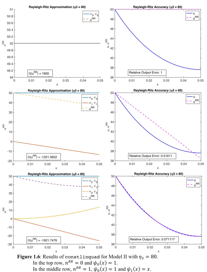
Results for 𝜂_K = 80 in Model II are shown in Figure 1.6 on the next page. For 𝑛FF _{= 0}

(top row of plots), relative output error is 100%, which is a very bad approximation. Remarkably, the approximation improves with 𝑛FF _{= 1 to 51.6% error and becomes quite good with 𝑛}FF _{= 2}

at 7.1% error. The observation that increasing the number of basis functions improves the approximation is another piece of evidence that Rayleigh-Ritz method is implemented correctly.

DISCUSSION

Overall Assessment of Code

Considering the implementation of exactinclude and constlinquad together

provides a unified means of assessing the accuracy of the code. According to the Minimization Proposition, Eq. (13), the energy functional is absolutely minimized when its argument, the candidate function, is the actual solution. In exactinclude, where the candidate function

contains the exact solution, the absolute minimum of the energy functional is found: Π(𝑢). On the other hand, in constlinquad, where the candidate function does not contain the exact solution,

the local minimum of the energy functional is found: Π(𝑢FF_{). A comparison of Π(𝑢}FF_{) and Π(𝑢)}

provides a metric by which to gauge the goodness of the Rayleigh-Ritz approximation:

• In Model I, Π(𝑢) = -10.13, while Π(𝑢FF_{) = -9.82, -10.31, and -10.31 for 𝑛}FF_{= 1, 2, and}

3, respectively. It is apparent that for 𝑛FF _{≥ 2, the Rayleigh-Ritz approximation achieves}

the actual solution because Π(𝑢FF_{) = Π(𝑢). Thus, two shape functions are sufficient to}

exactly represent Model I.

• In Model II, Π(𝑢) = -1927.19, while Π(𝑢FF_{) = 1600, -1221.57, and -1921.75 for 𝑛}FF_{= 0,}

1, and 2, respectively. As 𝑛FF_{increases, the Rayleigh-Ritz method better approximates the}

actual solution because Π(𝑢FF_{) approaches Π(𝑢). This agrees with the theory that as more}

shape functions are used, the energy functional decreases and the approximation improves. This assessment presents evidence of the successful implementation of the Rayleigh-Ritz method to model heat transfer through a conical frustum and right cylinder fin. These examples are among a large set of problems in engineering that have particular geometries and boundary conditions that make deriving analytical solutions difficult. The Rayleigh-Ritz method is the foundation of a

(10)

Figure 1.5: Results of constlinquad for Model I with 𝛽 = 0.

In the top row, 𝑛FF _{= 1 and 𝜓}

:(𝑥) = 1.

In the middle row, 𝑛FF _{= 2, 𝜓}

:(𝑥) = 1 and 𝜓,(𝑥) = 𝑥.

In the bottom row, 𝑛FF _{= 3, 𝜓}

:(𝑥) = 1, 𝜓,(𝑥) = 𝑥, and 𝜓K(𝑥) = 𝑥,. 0 0.02 0.04 0.06 0.08 0.1 x 24 24.2 24.4 24.6 24.8 25 25.2 25.4 25.6 25.8 26 u RR Rayleigh-Ritz Approximation ( = 0) 1 1 uRR (uRR) = -9.8175 0 0.02 0.04 0.06 0.08 0.1 x 25 30 35 40 45 u, u RR Rayleigh-Ritz Accuracy ( = 0) u uRR

Relative Output Error: 0.44444

0 0.02 0.04 0.06 0.08 0.1 x -30 -20 -10 0 10 20 30 40 50 u RR Rayleigh-Ritz Approximation ( = 0) 1 1 2 2 uRR (uRR) = -10.1316 0 0.02 0.04 0.06 0.08 0.1 x 25 30 35 40 45 50 u, u RR Rayleigh-Ritz Accuracy ( = 0) u uRR

Relative Output Error: 2.8422e-15

0 0.02 0.04 0.06 0.08 0.1 x -20 -10 0 10 20 30 40 50 u RR Rayleigh-Ritz Approximation ( = 0) 1 1 2 2 3 3 uRR (uRR) = -10.1316 0 0.02 0.04 0.06 0.08 0.1 x 25 30 35 40 45 u, u RR Rayleigh-Ritz Accuracy ( = 0) u uRR

(11)

Figure 1.6: Results of constlinquad for Model II with 𝜂K = 80.

In the top row, 𝑛FF _{= 0 and 𝜓} _{(𝑥) = 1.}

0 0.01 0.02 0.03 0.04 0.05 x 49 49.2 49.4 49.6 49.8 50 50.2 50.4 50.6 50.8 51 u RR Rayleigh-Ritz Approximation ( 3 = 80) 0 0 uRR (uRR) = 1600 0 0.01 0.02 0.03 0.04 0.05 x 36 38 40 42 44 46 48 50 u, u RR Rayleigh-Ritz Accuracy ( 3 = 80) u uRR

Relative Output Error: 1

0 0.01 0.02 0.03 0.04 0.05 x -20 -10 0 10 20 30 40 50 u RR Rayleigh-Ritz Approximation ( 3 = 80) 0 0 1 1 uRR (uRR) = -1221.5652 0 0.01 0.02 0.03 0.04 0.05 x 36 38 40 42 44 46 48 50 u, u RR Rayleigh-Ritz Accuracy ( 3 = 80) u uRR

0 0.01 0.02 0.03 0.04 0.05 x -30 -20 -10 0 10 20 30 40 50 u RR Rayleigh-Ritz Approximation ( 3 = 80) 0 0 1 1 2 2 uRR (uRR) = -1921.7476 0 0.01 0.02 0.03 0.04 0.05 x 36 38 40 42 44 46 48 50 u, u RR Rayleigh-Ritz Accuracy ( 3 = 80) u uRR

(12)

Model I 𝛽 Parameter

The parameter 𝛽 is the central angle (measured in radians) of the frustum in Model I. When 𝛽 = 0 the frustum is simply a right cylinder. The temperature profile is linear for 𝛽 = 0 (Eq. (5)),

and constlinquad has zero relative output error when 𝑛FF ≥ 2. When 𝛽 ≠ 0, the exact solution

(Eq. (4)) takes a shape that cannot be captured with 𝜓(𝑥) = 1, 𝑥, and 𝑥,_{(Figure 1.7). Therefore,}

the error of the Rayleigh-Ritz approximation increases as β increases and the temperature profile deviates from being linear (Table 1.1). Model I uses the Neumann/Robin boundary condition for one-dimensional problems. When 𝛽 is small, the approximation does well because heat transfer occurs primarily in the 𝑥-direction (quasi-1D); however, as 𝛽 increases, heat transfer in the other directions increases and the 1D model becomes less accurate.

Figure 1.7: Model I constlinquad for 𝛽 = 2.

The relative output error is larger at larger angles. Model II 𝜇+ Parameter

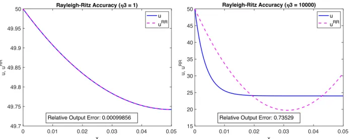
As defined by Eq. (10), 𝜇₊ is the non-dimensionalized fin parameter of Model II. 𝜇₊ describes a length factor over which the temperature changes in the fin, which is an important consideration when designing fins. For example, when 𝜇+ is on the order of 1 or smaller, the

temperature changes across the entire length of the fin, as shown in the left plot of Figure 1.8. Albeit in case shown, 𝜇₊ is too small for the fin to be an effective transferrer of heat, since ∆𝑢 < 0.3 °C. When 𝜇+ is much larger than 1, the temperature change occurs across only a portion of the

fin, as shown in the right plot of Figure 1.8. In this case, the entire length of the fin is not being utilizing, which may be a poor design choice.

The effect of 𝜇₊ on the accuracy of the Rayleigh-Ritz approximation can be investigated by holding the geometry and thermal conductivity of the fin constant and varying the heat transfer coefficient: thus 𝜇₊ is directly proportional to 𝜂_K. As shown in Table 1.2, the relative output error increases as 𝜇₊ increases. When 𝜇₊ is small, the exact solution has a parabola-like shape (note: it is actually a catenary) that the basis functions of constlinquad can approximate. The error in

the approximation is small. As 𝜇₊ increases, however, the catenary shape of the exact solution becomes more distinct, and the basis functions give a poor approximation. The error is large.

0 0.02 0.04 0.06 0.08 0.1 x 24 25 26 27 28 29 30 31 u, u RR Rayleigh-Ritz Accuracy ( = 2) u uRR

Table 1.1: 𝛽 effect on output error 𝛽 [rad] Relative output error [%]

0 0

0.5 0.045896

1 0.301

(13)

Figure 1.8: Model II constlinquad. In the left plot, 𝜇+ = 0.02 and the

Rayleigh-Ritz approximation has a small relative output error. In the right plot, 𝜇₊ = 200 and the approximation is inaccurate.

Table 1.2: 𝜂_K effect on output error 𝜂_K [W/m2 _°C] _𝜇

+ [/] Relative output error [%]

1 0.02 0.099856 80 1.6 7.1117 10000 200 73.529 0 0.01 0.02 0.03 0.04 0.05 x 49.7 49.75 49.8 49.85 49.9 49.95 50 u, u RR Rayleigh-Ritz Accuracy ( 3 = 1) u uRR

0 0.01 0.02 0.03 0.04 0.05 x 15 20 25 30 35 40 45 50 u, u RR Rayleigh-Ritz Accuracy ( 3 = 10000) u uRR

(14)

Chapter 2: The Finite Element Method for 1D 2nd-Order BVPs

ABSTRACT

In Chapter 2, finite element analysis is performed on Models I and II from Chapter 1 as well as a new Model Mine. The method is compared to the Rayleigh-Ritz method, with attention to the structure and advantage a new set of basis functions. Convergence of the approximate solution to the actual solution is tested and error estimators are considered. Finally, two theoretical models are discussed to further verify the finite element method.

INTRODUCTION

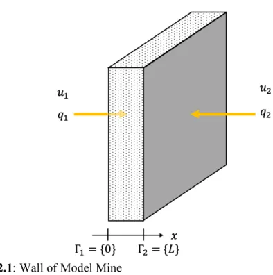
Chapter 2 builds upon Models I and II from the last chapter (see Chapter 1 for model descriptions). A new model, Model Mine, is also used, which describes 1D condition through a wall exposed to air temperatures and heat fluxes through the left and right surfaces (Figure 2.1).

Figure 2.1: Wall of Model Mine

The differential equation and boundary conditions for Model Mine are given by [4]_:

𝑑 𝑑𝑥(𝑘 𝑑𝑢 𝑑𝑥3 = 0 in 𝛺 (23) −𝑘𝑑𝑢 𝑑𝑥 = 𝜂:(𝑢 − 𝑢:) − 𝑞: on 𝛤: (24) −𝑘𝑑𝑢 𝑑𝑥 = 𝜂,(𝑢 − 𝑢,) − 𝑞, on 𝛤, (25) where the variables have the same assignments as Models I and II, with the exception of:

𝜂_: is the heat transfer coefficient between the left surface and the air [W/m2_°C]

(15)

𝑞_: is the heat flux through the left surface of the wall [W/m2_]

𝑞_, is the heat flux through the right surface of the wall [W/m2_]

𝑢_: is the ambient temperature on the left side of the wall [°C] 𝑢_, is the ambient temperature on the left side of the wall [°C] The exact solution to the wall problem is given by:

𝑢 = ‚𝜂:𝑞,− 𝜂_𝜂 ,𝑞:− 𝜂:𝜂,𝑢:+ 𝜂:𝜂,𝑢,

:𝑘 + 𝜂,𝑘 + 𝐿𝜂:𝜂, ƒ 𝑥

+ t𝑞:+ 𝑞,+ 𝜂,(𝑢,+ 𝐿(𝑞:+ 𝜂:𝑢:) 𝑘⁄ ) + 𝜂:𝑢: 𝜂_:+ 𝜂_,(1 + 𝐿𝜂_:⁄ )𝑘 u

(26)

Thus, the temperature within the wall follows a linear profile. The output of interest is

𝑠 ≡ 𝑢(𝑥 = 0), (27)

the temperature of the left surface of the wall.

BACKGROUND

Finite Element Method Formulation

The finite element method (FEM) is a numerical method used to analyze physical systems that can be modeled by partial differential equations subject to boundary conditions. Particularly in problems involving irregular geometry or composite materials, an analytical solution, 𝑢, may not exist. FEM produces an approximate solution, 𝑢_„, by dividing the domain into a mesh of elements at nodal positions, 𝑥h. The problem’s governing equations can be applied to these

elements. Union of the elements reproduces the domain and yields a system of equations, which FEM solves through an optimal combination of basis functions, 𝜑_h, and coefficients, 𝑢_„h [5]_:

𝑢_„(𝑥) = g 𝑢_„h 𝜑_h(𝑥)

a

hi:

(28) FEM is a special case of the Rayleigh-Ritz method in which the basis functions are piecewise linear (𝑝 = 1) or piecewise quadratic (𝑝 = 2) polynomials. In either case the basis function 𝜑_h(𝑥) for 1 ≤ 𝑖 ≤ 𝑛_a‡ˆ‰ is defined as:

𝜑_hP𝑥o_{Q = Š}1, 𝑗 = 1

0, 𝑗 ≠ 1 (29)

FEM maps a problem’s governing equations to general formulations. For a 1D 2nd_order

boundary value problem, the general differential equation is: − 𝑑

𝑑𝑥(𝜅(𝑥) 𝑑𝑢

𝑑𝑥3 + 𝜇(𝑥)𝑢 = 𝑓•(x) in 𝛺 (30)

The generalized boundary conditions are summarized in Table 2.1. The Neumann condition imposes a heat flux, the Robin condition describes convection by a heat transfer coefficient, and the Dirichlet condition specifies a fixed end temperature.

(16)

Table 2.1: Generalized boundary conditions for 1D 2nd_{order BVP}

End of domain Neumann-Robin boundary condition Dirichlet boundary condition

On 𝛤_: 𝜅(𝑥)𝑑𝑢_𝑑𝑥 = 𝛾:𝑢 − 𝑓•N 𝑢 = 𝑢•N

On 𝛤_, −𝜅(𝑥)𝑑𝑢

𝑑𝑥 = 𝛾,𝑢 − 𝑓•‘ 𝑢 = 𝑢•‘

An energy functional can be constructed from the general formulation: Π(𝑢_„) = 1 2m t𝜅(𝑥) ( 𝑑𝑢„ 𝑑𝑥 3 , + 𝜇(𝑥)𝑢_„,_{u 𝑑𝑥} n + +1 2P𝛾:𝑢„,(0) + 𝛾,𝑢„,(𝐿)Q − m 𝑓_•(𝑥)𝑢_„𝑑𝑥 n + − 𝑢_„(0)𝑓_M_N− 𝑢_„(𝐿)𝑓_M_‘ (31)

The coefficients of the approximate solution are found by minimizing the energy functional:

min 𝛱(𝑢„) → 𝐴 𝑢„ = 𝐹 (32)

where the elements of A and F are defined by: 𝐴_ho = m 𝜅(𝑥)𝜕𝜑h 𝜕𝑥 𝜕𝜑_o 𝜕𝑥 n + + 𝜇(𝑥)𝜑_h𝜑_o𝑑𝑥 + 𝛾_:𝜑_h(0)𝜑_o(0) + 𝛾_,𝜑_h(𝐿)𝜑_o(𝐿) 1 ≤ 𝑖, 𝑗 ≤ 𝑛 (33) 𝐹_h = m 𝑓_•(𝑥)𝜑_h𝑑𝑥 n + + 𝑓_M_N𝜑_h(0) + 𝑓_M_‘𝜑_h(𝐿) 1 ≤ 𝑖 ≤ 𝑛 (34) Implementation of Models

Solving Models I, II, and Mine with FEM follows a systematic workflow. Table 2.2 summarizes the types of boundary conditions imposed in the models. Each model’s governing equations are mapped to Eq. (30) and the generalized boundary conditions (see Table 2.3) [6]_.

Table 2.2: Types of boundary conditions in the models

End of domain Model I Model II Model Mine

On 𝛤_: Neumann Dirichlet Neumann-Robin

(17)

Table 2.3: Mapping models to generalized parameters

Parameter Heat transfer meaning Model I Model II Model Mine 𝜅(𝑥) Conductivity times area 𝑘𝜋𝑅₊,_{-1 + 𝛽}𝑥

𝐿1

,

𝑘𝐴_HI 𝑘𝐴

𝜇(𝑥) Heat transfer coefficient

times perimeter 0 𝜂K𝑃HI 0

𝑓_•(x) Generalized heat source 0 𝜂_K𝑃_HI𝑢_? 0

𝛾_: Generalized heat transfer

coefficient 0 − − 𝜂:𝐴

𝛾_, Generalized heat transfer _coefficient 𝜂_,𝜋𝑅₊,_{(1 + 𝛽)}, ₀ _𝜂 ,𝐴

𝑓_•_N Generalized heat flux 𝑞_:𝜋𝑅₊, _{− −} _(𝜂

:𝜇: + 𝑞:)𝐴

𝑓_•_‘ Generalized heat flux 𝜂_,𝜋𝑅₊,_{(1 + 𝛽)},_𝑢

? 0 (𝜂,𝜇, + 𝑞,)𝐴

𝑢•N Body temperature on 𝛤: − − 𝑢•N − −

𝑢_•_‘ Body temperature on 𝛤, − − − − − −

The elemental matrices 𝐴“_{and 𝐹}“_{are formed from the integral terms of Eq.s (33) and}

(34), where the superscript indicates that no boundary condition has been imposed. Each element is constructed through a mapping to a reference element that features the basis functions. Note: in implementation, a basis function is called a shape function and denoted 𝑠̂. The reference elements for 𝑝 = 1 and 𝑝 = 2 are shown in Figure 2.2.

Figure 2.2: Reference element for 𝑝 = 1 (left) [6]_{and 𝑝 = 2 (right)}[7]_.

Numerical quadrature is used to compute the integrals in 𝐴ho and 𝐹h. To impose the

boundary conditions, the remaining terms in Eq.s (33) and (34) are applied to 𝐴“_{and 𝐹}“_:

𝐴• = 𝐴“_{, but…} _𝐴•

:: = 𝐴•::+ 𝛾: 𝐴•a–—˜: a–—˜: = 𝐴•a–—˜: a–—˜:+ 𝛾,

(35) 𝐹™ = 𝐹“_{, but…} _𝐹™

: = 𝐹™:+ 𝑓•N 𝐹™a–—˜: = 𝐹™a–—˜:+ 𝑓•‘

(18)

in Model II, which imposes a left end Dirichlet condition, 𝐴, 𝐹, and a matrix 𝑏 are extracted from 𝐴• and 𝐹™ as shown in Figure 2.3. Then,

𝐴𝑢_„+ _{= 𝐹 − 𝑢}

•N𝑏 (36)

is solved for 𝑢_„+_{. Finally, 𝑢}

„ is formed from 𝑢„+ and 𝑢•N.

Figure 2.3: Extracting and forming matrices in a Dirichlet left end boundary condition [7]_.

The piecewise basis functions that characterize FEM have special features. Firstly, a coefficient at node i is physically meaningful: it is exactly the estimate of 𝑢 at that node, since 𝑢„(𝑥h) = 𝑢_„h. In Models I and Mine, FEM immediately outputs nodal temperatures in computing

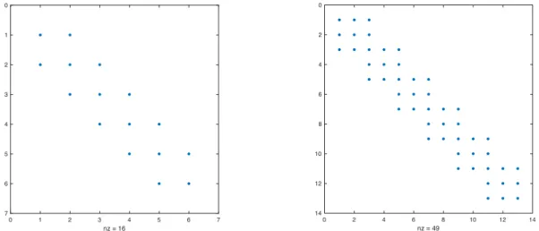
the coefficients. Secondly, the A matrix is sparse. It is tridiagonal for 𝑝 = 1 and pentadiagonal for 𝑝 = 2, which makes FEM is computationally efficient.

RESULTS Model II Results

The output of Model II is shown in Figure 2.4. Notice that in the top row, the left plot shows that the finite element (FE) solution is composed of piecewise continuous linear polynomials (𝑝 = 1) and its derivative is disjointed flat lines. After six uniform refinements, the FE solution is not visibly distinguishable from the actual solution, suggesting convergence. Similar observations can be made for 𝑝 = 2 in the bottom row of plots; note the piecewise quadratic polynomials in the FE solution and the linear polynomials in the FE derivative. Another verification of successful FEM implementation is that the error converges at the expected rates (to be discussed in Model II Error Analysis). The results of Model II provide confidence that

form_elem_mat_sver[8], the code that constructs the elemental matrices, is working properly

since Model II has nonzero boundary parameters 𝜇(𝑥) and 𝑓_•(x). Furthermore, matrix A has the expected sparsity pattern (Figure 2.5).

(19)

Figure 2.4: Model II Results (𝑝 = 1 in top row and 𝑝 = 2 in bottom row).

Figure 2.5: Cropped sections of matrix A of Model II to visualize sparsity pattern. Note that for 𝑝 = 1 A is tridiagonal and for 𝑝 = 2 A is pentadiagonal, as expected.

0 0.02 0.04 0.06 x 15 20 25 30 35 40 45 50 field Mesh 0 FE exact 0 0.02 0.04 0.06 x -8 -7 -6 -5 -4 -3 -2 -1 0 1 derivative of field 104 Mesh 0 FE exact 0 0.02 0.04 0.06 x 15 20 25 30 35 40 45 50 field Mesh 0 FE exact 0 0.02 0.04 0.06 x -8 -7 -6 -5 -4 -3 -2 -1 0 1 derivative of field 104 Mesh 0 FE exact 0 1 2 3 4 5 6 7 nz = 16 0 1 2 3 4 5 6 7 0 2 4 6 8 10 12 14 nz = 49 0 2 4 6 8 10 12 14

(20)

Model I Results

The output of Model I is shown in Figure 2.6. The convergence of 𝑢„ to 𝑢 is evident by

the improvement of the FE solution from Mesh 0 to Mesh 6. For Model I, 𝑝 = 2 is particularly effective at capturing the derivative solution. The results of Model I provide confidence that

impose_boundary_cond_sver[9], the code that implements Eq. (35), is working properly since

Model I has nonzero boundary parameters 𝛾,, 𝑓•N, and 𝑓•‘.

Figure 2.6: Model I results (𝑝 = 1 in top row and 𝑝 = 2 in bottom row). Model Mine Results

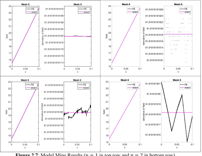
The output of Model Mine is shown in Figure 2.7. Since the exact solution of Model Mine is linear, the FE solution with 𝑝 = 1 captures the exact solution on Mesh 0. An interesting phenomenon occurs with further refinement. Because the finite precision of computer computation can only represent numbers to a finite precision (14 digits), the error in the approximation appears to increase with further refinement because the finite precision is compounded (Figure 2.8). This artifact is also evident from the strange-looking plots of the FE derivative in Figure 2.7; note the scale of the vertical axis.

Model Mine provides greater confidence of correct FEM implementation than Model I because Model Mine has complete boundary conditions (heat flux and convection) at both ends of the domain; i.e. 𝛾_:, 𝛾_,, 𝑓_•_N, and 𝑓_•_‘ are nonzero. In contrast, 𝛾_: = 0 in Model I, and an

0 0.05 0.1 x 24 25 26 27 28 29 30 field Mesh 0 FE exact 0 0.05 0.1 x -200 -180 -160 -140 -120 -100 -80 -60 -40 -20 0 derivative of field Mesh 0 FE exact 0 0.05 0.1 x 24 25 26 27 28 29 30 field Mesh 0 FE exact 0 0.05 0.1 x -200 -180 -160 -140 -120 -100 -80 -60 -40 -20 0 derivative of field Mesh 0 FE exact

(21)

implementation error in impose_boundary_cond_sver involving 𝛾: could go unnoticed when

analyzing Model I. Such a bug would be detected when running Model Mine.

Figure 2.7: Model Mine Results (𝑝 = 1 in top row and 𝑝 = 2 in bottom row).

0 0.05 0.1 x 15 16 17 18 19 20 21 22 23 24 field Mesh 0 FE exact 0 0.05 0.1 x 81.818181818174 81.818181818176 81.818181818178 81.81818181818 81.818181818182 81.818181818184 81.818181818186 81.818181818188 81.81818181819 derivative of field Mesh 0 FE exact 0 0.05 0.1 x 15 16 17 18 19 20 21 22 23 24 field Mesh 0 FE exact 0 0.05 0.1 x 81.818181818174 81.818181818176 81.818181818178 81.81818181818 81.818181818182 81.818181818184 81.818181818186 81.818181818188 81.81818181819 derivative of field Mesh 0 FE exact 1 1.5 2 2.5 -log10(h_max/L) -19 -18 -17 -16 -15 -14 -13 -12 -11 log 10 (error in H 1 norm) error error estimate line of slope -1 1 1.5 2 2.5 -log10(h_max/L) -19 -18 -17 -16 -15 -14 -13 -12 -11 log 10 (error in L 2 norm) error error estimate line of slope -2 1 1.5 2 2.5 -log10(h_max/L) -19 -18 -17 -16 -15 -14 -13 -12 -11 log 10 (error in L norm) error error estimate line of slope -1.5 1 1.5 2 2.5 -log10(h_max/L) -19 -18 -17 -16 -15 -14 -13 -12 -11 log 10 (error in output) error error estimate line of slope -2 1 1.5 2 2.5 -log10(h_max/L) -25 -20 -15 -10 log 10 (error in H 1 norm) error error estimate line of slope -2 1 1.5 2 2.5 -log10(h_max/L) -25 -20 -15 -10 log 10 (error in L 2 norm) error error estimate line of slope -3 1 1.5 2 2.5 -log10(h_max/L) -25 -20 -15 -10 log 10 (error in L norm) error error estimate line of slope -2.5 1 1.5 2 2.5 -log10(h_max/L) -25 -20 -15 -10 log 10 (error in output) error error estimate line of slope -4

(22)

Model II Error Analysis

The more accurate the FE approximation, the more time the algorithm takes to run. This tradeoff is balanced when FEM refines just until numerical specifications are met. Error in the approximation can be found by comparing the FE solution to the actual solution, which is known as a priori error estimation. However, how can the error be found when the exact solution is not known? A posteriori error estimators derive estimates of the error using just the FE solution by comparing 𝑢_„ to 𝑢_„/,, the estimate after a refinement. Common error estimators are summarized in Table 2.4. The exponent of the bound, the convergence rate, is the absolute value of the slope on a log(error) vs. log(L/h) plot. Checking that the error converges at the expected rate is a good verification technique.

Table 2.4: FE error estimators [10]

Description Definition A priori error

estimator

Bound A posteriori error

estimator A norm reflecting temperature and its gradient ‖𝑣‖_•N_(•)= m (𝑑𝑣 𝑑𝑥3 , +𝑣, 𝐿 𝑑𝑥 n + ž𝑢 − 𝑢„/,ž_•N_(•) ~𝐶_¡-„ ,1 ¢ _≤ž𝑢„/,− 𝑢„ž•N_(•) 2¢ _{− 1} A norm reflecting temperature ‖𝑣‖n‘(•)= m 𝑣 ,_𝑑𝑥 n + ž𝑢 − 𝑢„/,ž_n‘_(•) ~𝐶_¡-„ ,1 ¢˜: _≤ž𝑢„/,− 𝑢„žn‘(•) 2(¢˜:)_{− 1} A norm reflecting maximum temperature over domain ‖𝑣‖_n£_(•)= max|𝑣| ž𝑢 − 𝑢_„/,ž n£_(•) ~𝐶_¡-„ ,1 ¢˜:/, ≤ž𝑢„/,₂_(¢˜:/,)− 𝑢„ž_{− 1}n£(•) The problem’s output 𝑠 ¥𝑠 − 𝑠„/,¥ ~𝐶¡ -„ ,1 ,¢ ≤¥𝑠„/,− 𝑠„¥ 2,¢ _{− 1}

To realistically assess the accuracy of the FE solution, Model II was studied on a sequence of 9 meshes (8 refinements) for 𝑝 = 1 without reference to the exact solution. Error plots are shown in Figure 2.9. What do these plots convey about the minimum necessary refinements to achieve a numerical specification? Two criteria must be met to achieve a desired accuracy most efficiently. The first criterion says that convergence is uncertain until error in the 𝐻:_{(Ω) norm}

decreases with further refinement. The second criterion says that the error in the output or a chosen norm must be less than a numerical specification.

(23)

Figure 2.9: Estimated error in Model II (𝑝 = 1) without reference to the exact error. For example, say that ‖𝑢 − 𝑢„‖n£_(•) must be less than 1.00. On a log scale, the error is

then less than 0. From the 𝐻:_{(Ω) plot in Figure 2.9, it is evident that first criterion is not satisfied}

until Mesh 5 (the fourth point). Then, from the 𝐿?_{(Ω) plot, the coarsest mesh that satisfies}

log‖𝑢 − 𝑢_„‖_n£_(•) < 0 can be identified as Mesh 7 (the sixth point). Mesh 7 is finer than Mesh 5,

so both criteria are met. On Mesh 7, log‖𝑢 − 𝑢_„‖_n£_(•) = −0.1967. Then the error in the 𝐿?(Ω)

norm is 10«+.:¬-® _{= 0.6358. In practice the higher order contributions to the error bound should}

be accounted for by including a safety factor. If SF=2, the upper bound for error in the 𝐿?_(Ω)

norm is 1.2715, which does not meet specification. Thus, one further refinement is necessary for the prediction to be sufficiently accurate. On Mesh 8, log‖𝑢 − 𝑢„‖n£_(•) = −0.7126. Then the

upper bound for the error in the 𝐿?_{(Ω) norm is 2 ∗ 10}«+.®:,- _{= 0.3876, which is within}

specification.

As another example, consider the upper bound for the error in the output on Mesh 5. log|𝑠 − 𝑠_„| = 1.443 on Mesh 5, so |𝑠 − 𝑠_„| = 10:.´´K _{= 27.73. If SF=2, then the error in the}

output on Mesh 5 has an upper bound of 55.47.

Since the exact solution to Model II is known, the actual errors can be found. As shown in Figure 2.10, the a posteriori error estimators are quite good, and a safety factor of 2 is not necessary. This is also evident in Table 2.5. However, when the actual error is unknown, a finer mesh that may be required by including a safety factor is worth the higher confidence in accuracy.

Table 2.5: Error comparison

‖𝑢 − 𝑢 ‖ on Mesh 8 |𝑠 − 𝑠 | on Mesh 5 1.5 2 2.5 3 -log10(h_max/L) -6 -5 -4 -3 -2 -1 0 1 2 3 log 10 (error in H 1 norm) error estimate line of slope -1 1.5 2 2.5 3 -log10(h_max/L) -6 -5 -4 -3 -2 -1 0 1 2 3 log 10 (error in L 2 norm) error estimate line of slope -2 1.5 2 2.5 3 -log10(h_max/L) -6 -5 -4 -3 -2 -1 0 1 2 3 log 10 (error in L norm) error estimate line of slope -1.5 1.5 2 2.5 3 -log10(h_max/L) -6 -5 -4 -3 -2 -1 0 1 2 3 log 10 (error in output) error estimate line of slope -2

(24)

Figure 2.10: Estimated and exact errors in Model II (𝑝 = 1).

DISCUSSION

Method of Manufactured Solutions

Convergence of 𝑢_„ to 𝑢 at the correct rate does not necessarily prove that the code

form_elem_mat_sver is bug-free for all possible instantiations of 𝜇(𝑥). For example, 𝜇(𝑥) may

not be a constant, such as when the perimeter of a fin depends on 𝑥. Let’s define a new model that describes a conical frustum-shaped fin with constant temperature on its left surface and zero heat flux through its right surface, such that 𝜇(𝑥) = 2𝜋𝑅+-1 +µ_n1 𝜂,, 𝜅(𝑥) = 𝑘𝜋𝑅+,-1 +µ_n1

,

, and 𝛾, = 0. Using the method of manufactured solutions [10], say 𝑢 = 𝛼𝑥,. From Eq. (32), then:

𝑓_•(𝑥) = − 𝑑 𝑑𝑥(𝜅 𝑑𝑢 𝑑𝑥3 + 𝜇(𝑢 − 𝑢?) = −2𝛼𝑘𝜋𝑅₊,_{¶1 +}4𝑥 𝐿 + 3𝑥, 𝐿, · + 2𝜋𝑅+(1 + 𝑥 𝐿)𝜂,(𝛼𝑥,− 𝑢?) (37)

Then the model’s differential equation and boundary conditions are: − 𝑑 𝑑𝑥(𝑘𝜋𝑅+,-1 + 𝑥 𝐿1 ,_𝑑𝑢 𝑑𝑥3 + 2𝜋𝑅+(1 + 𝑥 𝐿)𝜂,𝑢 = −2𝛼𝑘𝜋𝑅₊,_{¶1 +}4𝑥 𝐿 + 3𝑥, 𝐿, · + 2𝜋𝑅+(1 + 𝑥 𝐿)𝜂,(𝛼𝑥,− 𝑢?) in 𝛺 (38) 𝑢 = 𝑢_M_N on 𝛤_: (39) −4𝑘𝜋𝑅₊,𝑑𝑢 𝑑𝑥 = 𝑓•‘ on 𝛤, (40) 1 2 3 -log10(h_max/L) -6 -5 -4 -3 -2 -1 0 1 2 3 log 10 (error in H 1 norm) error error estimate line of slope -1 1 2 3 -log10(h_max/L) -6 -5 -4 -3 -2 -1 0 1 2 3 log 10 (error in L 2 norm) error error estimate line of slope -2 1 2 3 -log10(h_max/L) -6 -5 -4 -3 -2 -1 0 1 2 3 log 10 (error in L norm) error error estimate line of slope -1.5 1 2 3 -log10(h_max/L) -6 -5 -4 -3 -2 -1 0 1 2 3 log 10 (error in output) error error estimate line of slope -2

(25)

Since 𝑢 is known, the FE solution to this model can be validated, providing additional confidence that form_elem_mat_sver is correctly implemented.

Model X

In a theoretical Model X the exact solution is not known. Running the FE code, it is observed that for sufficiently small ℎ the extrapolation error estimators converge at the anticipated rates in all norms. Can it be concluded that 𝑢_„ converges to the exact solution 𝑢 of Model X? No, it cannot, due to the possibility of implementation error.

There are three potential sources of error when running FEM. One type of error comes from the model itself. Is the mathematical model sufficiently detailed to capture the physics of the system? Another type of error comes from numerical specification. Are the FEM parameters, such as mesh size and basis polynomial order, tuned to meet the required specification? Numerical specification was explored in Model II Error Analysis. Lastly, there may be implementation error. Model Mine Results demonstrated that there is inherent implementation error due to the finite precision of computer computation. However, implementation error can be more consequential when the code is not implemented correctly. There could be typos in imputing the model’s, such as omitting a negative sign or mistaking a decimal place, or the code could run the wrong model. For example, run_uniform_refinement[11] features four models. It could be easy to confuse

the results of one model for another without attention what section the code is running or an intuition of the model’s solution. Model X could be prone to these human implementation errors.

(26)

Chapter 3: Time Dependent Finite Element Method for 1D 2nd-Order BVPs

ABSTRACT

In Chapter 3, the finite difference tool is added the finite element method to study time-dependent problems. A simple model of a semi-infinite fin is first analyzed to provide confidence that the method is implemented correctly. Then a more complicated model describing cooking a burger is analyzed. A recipe for “Tender, Juicy Grilled Burgers” from Cook’s Illustrated is implemented to assess the predictability of the model.

INTRODUCTION

Model Semiinf_plus describes the transfer of heat through a right-cylinder fin at an initial uniform temperature and experiencing convection on its left surface and zero heat transfer

through its right surface (Figure 3.1).

Figure 3.1: Fin geometry of Model Semiinf_plus.

The differential equation, boundary conditions, and initial condition are given by [12]_:

𝜌𝑐𝐴𝜕𝑇 𝜕𝑡 = 𝑘A 𝜕2_𝑇 𝜕𝑥2+ 𝜂½¾¿𝑃(𝑇 − 𝑇?) 0 ≤ 𝑥 ≤ 𝐿, 0 < 𝑡 ≤ 𝑡À (41) 𝑘𝐴𝜕𝑇 𝜕𝑥 = 𝜂Á‡¿A(𝑇 − 𝑇?) 𝑥 = 0, 0 < 𝑡 ≤ 𝑡À (42) −𝑘𝐴𝜕𝑇 𝜕𝑥= 0 𝑥 = 𝐿, 0 < 𝑡 ≤ 𝑡À (43) 𝑇 = 𝑇_hH 0 ≤ 𝑥 ≤ 𝐿, 𝑡 = 0 (44) where:

𝐿 is the length of the body [m]

𝐴 is the cross sectional area of the body [m2_]

𝑃 is the cross sectional perimeter of the body [m] 𝜌𝑐 is the volumetric specific heat [J/m3_°C]

𝑘 is the thermal conductivity of the body [W/m °C]

𝜂_½¾¿ is the heat transfer coefficient between the lateral surface and the air [W/m2_°C]

(27)

𝑇_? is the ambient temperature [°C]

𝑇(𝑥, 𝑡) is the spatial and temporal temperature profile of the body [°C]

Model Burger describes cooking a burger on a skillet (Figure 3.2). Cooking the burger involves three stages: Stage I (pre-flip) from 0 ≤ 𝑡 ≤ 𝑡Â_{, during which side 𝛼 cooks; Stage II}

(post-flip) from 𝑡Â _{≤ 𝑡 ≤ 𝑡}ÂÂ_{, during which side}_{𝛽 cooks; and Stage III (repose) from 𝑡}ÂÂ _{≤ 𝑡 ≤ 𝑡}ÂÂÂ_,

during which the burger cools on a rack.

Figure 3.2: Geometry of Model Burger

The differential equation, boundary conditions, and initial condition of the burger problem for the three stages are summarized in Table 3.1.

Table 3.1: Model Burger governing equations

Stage I (0 ≤ 𝑡 ≤ 𝑡Â₎ _{Stage II (𝑡}Â _{≤ 𝑡 ≤ 𝑡}ÂÂ₎ _{Stage III (𝑡}ÂÂ_{≤ 𝑡 ≤ 𝑡}ÂÂÂ₎ _{On domain}

𝜌𝑐𝐴𝜕𝑇 Â 𝜕𝑡 = 𝑘A𝜕,𝑇Â 𝜕𝑥, + 𝜂½¾¿Â 𝑃(𝑇Â− 𝑇?) 𝜌𝑐𝐴𝜕𝑇 ÂÂ 𝜕𝑡 = 𝑘A𝜕,𝑇ÂÂ 𝜕𝑥, + 𝜂½¾¿ÂÂ 𝑃(𝑇ÂÂ− 𝑇?) 𝜌𝑐𝐴𝜕𝑇 ÂÂÂ 𝜕𝑡 = 𝑘A𝜕,𝑇ÂÂÂ 𝜕𝑥, + 𝜂½¾¿ÂÂÂ𝑃(𝑇ÂÂÂ− 𝑇?) 0 < 𝑥 < 𝐿 𝑘𝐴𝜕𝑇_𝜕𝑥Â = 𝜂Á‡¿Â 𝐴(𝑇Â− 𝑇IÃh½½‰¿) 𝑘𝐴𝜕𝑇_𝜕𝑥ÂÂ = 𝜂Á‡¿ÂÂ 𝐴(𝑇ÂÂ− 𝑇IÃh½½‰¿) 𝑘𝐴𝜕𝑇_𝜕𝑥ÂÂÂ= 𝜂Á‡¿ÂÂÂ 𝐴(𝑇ÂÂÂ− 𝑇?) 𝑥 = 0 −𝑘𝐴𝜕𝑇_𝜕𝑥Â = 𝜂¿‡¢Â 𝐴(𝑇Â− 𝑇?) −𝑘𝐴𝜕𝑇_𝜕𝑥ÂÂ= 𝜂¿‡¢ÂÂ 𝐴(𝑇ÂÂ− 𝑇?) −𝑘𝐴𝜕𝑇_𝜕𝑥ÂÂÂ= 𝜂¿‡¢ÂÂÂ 𝐴(𝑇ÂÂÂ− 𝑇?) 𝑥 = 𝐿 𝑇Â_{(𝑥, 0) = 𝑇} hH 𝑇ÂÂ(𝑥, 𝑡Â) = 𝑇Â(𝐿 − 𝑥, 𝑡Â) 𝑇ÂÂÂ(𝑥, 𝑡ÂÂ) = 𝑇ÂÂ(𝑥, 𝑡ÂÂ) 0 < 𝑥 < 𝐿 where:

𝐿 is the burger thickness [m]

𝐴 is the burger cross sectional area [m2_]

𝑃 is the burger cross sectional perimeter [m] 𝜌𝑐 is the burger volumetric specific heat [J/m3_°C]

𝑘 is the burger thermal conductivity [W/m °C]

𝜂_½¾¿ is the heat transfer coefficient on the lateral surface [W/m2_°C]

𝜂_¿‡¢ is the heat transfer coefficient on the top surface [W/m2_°C]

(28)

BACKGROUND

Formulation of the Heat Equation

The solution to the heat equation is a temperature profile, 𝑢, that depends on time and space. The spatial component is approximated by the finite element (FE) method, which divides the domain into a mesh of 𝑛_‰½ elements of length ℎ. The temporal component is approximated by the finite difference (FD) method, which discretizes time into 𝑛_¿I¿‰¢I steps of duration ∆𝑡. Just as the FE method can implement different basis functions, most notably piecewise linear (𝑝 = 1) and piecewise quadratic (𝑝 = 2), the FD method invokes different schemes (𝜃) to approximate time-dependent derivatives. Three common schemes are summarized in Table 3.2. This analysis utilizes the Euler backward and Crank-Nicolson schemes because they are convergent and stable. They are also less numerically costly than Euler forward, which requires much smaller time steps to reach a desired accuracy.

Table 3.2: Finite difference schemes

𝜃 Name Rule implemented Characteristics in time 0 Euler forward Rectangle right 1st_{order, explicit, unstable}

1/2 Crank-Nicolson Trapezoidal 2nd_{order, implicit, stable}

1 Euler backward Rectangle left 1st_{order, implicit, stable}

The FD-FE method approximates the solution to the heat equation in both time and space. The heat equation and N/R-N/R boundary conditions, applicable to Models Semiinf_Plus and Burger, take the form [13]_:

− 𝜕 𝜕𝑥(𝜅(𝑥) 𝜕𝑢 𝜕𝑥3 + 𝜇(𝑥)𝑢 = 𝑓•− 𝜌(𝑥)𝑢̇ in 𝛺, 0 < 𝑡 ≤ 𝑡À (45) 𝜅𝜕𝑢 𝜕𝑥 = 𝛾:𝑢 − 𝑓MN on 𝛤:, 0 < 𝑡 ≤ 𝑡À (46) −𝜅𝜕𝑢 𝜕𝑥= 𝛾,𝑢 − 𝑓M‘ on 𝛤,, 0 < 𝑡 ≤ 𝑡À (47) 𝑢 = 𝑢_hH(𝑥) in 𝛺, 𝑡 = 0 (48)

The FD-FE solution to the heat equation is:

𝑢_„,∆¿Ã _{(𝑥), 1 ≤ 𝑘 ≤ 𝑛}

¿I¿‰¢I (49)

𝑢_„,∆¿Ã _{(𝑥), a numerical approximation to the true solution 𝑢(𝑥, 𝑡), is found by solving:}

𝑀ha‰Ç¿h¾𝑢„,∆¿Ã − 𝑢„,∆¿Ã«:

∆𝑡 + 𝐴P𝜃𝑢„,∆¿Ã − (1 − 𝜃)𝑢„,∆¿Ã«:Q = 𝐹 , 2 ≤ 𝑘 ≤ 𝑛¿I¿‰¢I

𝑢_„,∆¿Ã _{= 𝐼}

„𝑢hH , 𝑘 = 1

(50) where the elemental matrices are defined by the parameters of the boundary value problem:

𝑀_hoha‰Ç¿h¾ _{= m 𝜌(𝑥)𝜑} h𝜑o𝑑𝑥 n + 1 ≤ 𝑖, 𝑗 ≤ 𝑛 (51) 𝐴_ho = m 𝜅(𝑥)𝜕𝜑h 𝜕𝑥 𝜕𝜑_o 𝜕𝑥 n + + 𝜇(𝑥)𝜑_h𝜑_o𝑑𝑥 + 𝛾_:𝜑_h(0)𝜑_o(0) + 𝛾_,𝜑_h(𝐿)𝜑_o(𝐿) 1 ≤ 𝑖, 𝑗 ≤ 𝑛 (52)

(29)

𝐹h = m 𝑓•(𝑥)𝜑h𝑑𝑥 n

+

+ 𝑓MN𝜑h(0) + 𝑓M‘𝜑h(𝐿) 1 ≤ 𝑖 ≤ 𝑛 (53)

Implementation of Models

To solve the Semiinf_plus and Burger problems, the models’ boundary value equations are mapped to Eq.s (45)-(47), which is summarized in Table 3.3. The code

run_uniform_refinement solves Eq. (50) for 𝑢_„,∆¿Ã (𝑥).

Table 3.3: Mapping models to generalized parameters Parameter Heat transfer meaning Value in Model

Semiinf_plus

Value in Model Burger

pre-flip (I), post-flip (II), repose (III) 𝜌(𝑥) Density times specific _{heat times area} 1 𝜌𝑐𝐴

𝜅(𝑥) Conductivity times _area 1 𝑘𝐴

𝜇(𝑥) coefficient times Heat transfer perimeter

1

𝜂_½¾¿Â _𝑃

𝜂_½¾¿ÂÂ _𝑃

𝜂_½¾¿ÂÂÂ_𝑃

𝑓_•(x) Generalized heat _source 0

𝜂_½¾¿Â _𝑃𝑇 ? 𝜂_½¾¿ÂÂ _𝑃𝑇 ? 𝜂_½¾¿ÂÂÂ_𝑃𝑇 ?

𝛾_: _{transfer coefficient}Generalized heat 1

𝜂_Á‡¿Â _𝐴

𝜂_Á‡¿ÂÂ _𝐴

𝜂_Á‡¿ÂÂÂ _𝐴

𝛾, _{transfer coefficient}Generalized heat 0

𝜂_¿‡¢Â _𝐴

𝜂_¿‡¢ÂÂ _𝐴

𝜂_¿‡¢ÂÂÂ _𝐴

𝑓_•_N Generalized heat flux 0

𝜂_Á‡¿Â _𝐴𝑇 IÃh½½‰¿ 𝜂_Á‡¿ÂÂ _𝐴𝑇 IÃh½½‰¿ 𝜂_Á‡¿ÂÂÂ _𝐴𝑇 ?

𝑓_•_‘ Generalized heat flux 0

𝜂_¿‡¢Â _𝐴𝑇 ? 𝜂_¿‡¢ÂÂ _𝐴𝑇 ? 𝜂_¿‡¢ÂÂÂ _𝐴𝑇 ?

(30)

RESULTS

Verification of Model Semiinf_plus Implementation

The output of Model Semiinf_plus is shown in Figure 3.3. The convergence of the FE solution, 𝑢_„,∆¿Ã _{(𝑥), to the exact solution, 𝑢(𝑥, 𝑡}Ã_{), is evident by the improvement of fit from Mesh}

0 to Mesh 3. Observe that the 𝑝 = 2 scheme does a better job capturing the solution at fewer refinements than the 𝑝 = 1 scheme, and it is much more effective at capturing the derivative solution.

Figure 3.3: Model Semiinf_plus results (Top row: 𝑝 = 1 and 𝜃 = 1; Bottom row: 𝑝 = 2 and 𝜃 = 1/2).

With each refinement, the FD-FE method divides ℎ by a factor of 2 and ∆𝑡 by a factor of 𝜎, which is chosen such that FD and FE approximations converge at the same rate [14]_{. The}

convergence rate for 𝐿,_{(Ω) is ~𝐶}

¡,Ê2«Ç½, where 𝐶¡,Ê is the sum of the spatial and temporal

convergence constants, 𝑙 is the refinement level, and 𝑟 is the convergence rate. For the 𝐿,_{(Ω) norm,}

𝑟 = 𝑝 + 1. As seen by the negative slope in the error estimators plotted in Figure 3.4, the solution converges at the expected rates, giving confidence that the code solve_fld_output_t_sver[15]

is implemented correctly. 0 0.5 1 x 0.84 0.86 0.88 0.9 0.92 0.94 0.96 0.98 1 field Mesh 0 FE exact 0 0.5 1 x -0.1 0 0.1 0.2 0.3 0.4 0.5 0.6 0.7 0.8 0.9 derivative of field Mesh 0 FE exact 0 0.5 1 x 0.84 0.86 0.88 0.9 0.92 0.94 0.96 0.98 1 field Mesh 3 FE exact 0 0.5 1 x 0 0.1 0.2 0.3 0.4 0.5 0.6 0.7 0.8 0.9 derivative of field Mesh 3 FE exact 0 0.5 1 x 0.84 0.86 0.88 0.9 0.92 0.94 0.96 0.98 1 field Mesh 0 FE exact 0 0.5 1 x -0.1 0 0.1 0.2 0.3 0.4 0.5 0.6 0.7 0.8 0.9 derivative of field Mesh 0 FE exact 0 0.5 1 x 0.84 0.86 0.88 0.9 0.92 0.94 0.96 0.98 1 field Mesh 3 FE exact 0 0.5 1 x -0.1 0 0.1 0.2 0.3 0.4 0.5 0.6 0.7 0.8 0.9 derivative of field Mesh 3 FE exact

(31)

Figure 3.4: Model Semiinf_plus 𝐿,_{(Ω) norm error estimators (Left: 𝑝 = 1 and}

𝜃 = 1; Right 𝑝 = 2 and 𝜃 = 1/2). Verification of Model Burger Implementation

Key results of Model Burger are shown in Figure 3.5. The content of these plots is explored in the Discussion. For now, the interest is verification of correct implementation, which is done by direct comparison. The top row of Figure 3.5 shows results obtained from the code

run_uniform_refinement_burger_sver[16], where the function make_probdef_burger

was modified with the burger parameters shown in Table 3.3. In comparison, the bottom row of Figure 3.5 shows results reported by AT Patera [17]_{. Using MATLAB’s interactive data cursor,}

precise comparisons can be made on selected points. This test is a basic demonstration of the common technique of verifying the implementation of a code, such as that used for this project, by comparing its results to the results of rigorously developed commercial software.

Verification of Model Burger Numerical Specifications

Error estimators of the output—the burger temperature 𝑇Â_{at the skillet side at time 𝑡}Â_just

before the flip—are shown in Figure 3.6. For the output error, 𝑟 = 2𝑝. As an exercise, say the error is specified to be less than 0.001 °C (less than -3 on a logarithmic scale). A safety factor of 1 is sufficient for a burger. Then, for 𝑝 = 1 and 𝜃 = 1, the coarsest mesh that meets the prescribed tolerance is Mesh 6 (fifth refinement) with coordinates (2.283, -3.443). The tolerance is thus 10«K.´´K _{= 0.00036 °C. Mesh 6 is circled in red on the left plot of Figure 3.6. For 𝑝 = 2 and 𝜃 =}

1/2, the coarsest mesh that meets the prescribed tolerance appears to be Mesh 2 (first refinement) with coordinates (1.079, -3.273). However, there is a special caveat for this particular scheme. Note, the slope of the data in the right plot is -3 instead of -4. The output error of a FD-FE second order scheme convergences at a rate of ~𝐶_¡,Ê2«(Ç«:)½_{. Thus, it is good practice to create an upper}

bound on the error by scaling by a factor of 2, which shifts the data points up by log(2) = 0.301. Then, −3.273 + 0.301 = −2.972 > −3, and Mesh 2 does not achieve specification. Conversely, Mesh 3 (second refinement) with coordinates (1.38, -4.175) does meet specification because

0.8 1 1.2 1.4 1.6 -log10(h_max/L) -7 -6 -5 -4 -3 -2 log 10 (error in H 1 norm) error error estimate line of slope -1 0.8 1 1.2 1.4 1.6 -log10(h_max/L) -7 -6 -5 -4 -3 -2 log 10 (error in L 2 norm) error error estimate line of slope -2 0.8 1 1.2 1.4 1.6 -log10(h_max/L) -7 -6 -5 -4 -3 -2 log 10 (error in L norm) error error estimate line of slope -1.5 0.8 1 1.2 1.4 1.6 -log10(h_max/L) -7 -6 -5 -4 -3 -2 log 10 (error in output) error error estimate line of slope -2 0.8 1 1.2 1.4 1.6 -log10(h max/L) -11 -10 -9 -8 -7 -6 -5 -4 -3 log 10 (error in H 1 norm) error error estimate line of slope -2 0.8 1 1.2 1.4 1.6 -log10(h max/L) -11 -10 -9 -8 -7 -6 -5 -4 -3 log 10 (error in L 2 norm) error error estimate line of slope -3 0.8 1 1.2 1.4 1.6 -log10(h max/L) -11 -10 -9 -8 -7 -6 -5 -4 -3 log 10 (error in L norm) error error estimate line of slope -2.5 0.8 1 1.2 1.4 1.6 -log10(h max/L) -11 -10 -9 -8 -7 -6 -5 -4 -3 log 10 (error in output) error error estimate line of slope -4

(32)

Figure 3.5: Verification of Model Burger implementation using the data cursor. Top row: Results obtained from FEM. Bottom row: Results reported by AT Patera.

Figure 3.6: Model Burger output error estimators (Left: 𝑝 = 1 and 𝜃 = 1; Right 𝑝 = 2 and 𝜃 = 1/2).

0 100 200 300 400 500 600 700 800 900 time (in seconds)

0 20 40 60 80 100 120 140 160 180 200

temperature (in degrees Celsius)

Flipping 2.S976 Burgers

burger temperature: skillet side burger temperature: air side burger temperature: mid-burger initial burger temperature room temperature serve temperature done temperature Maillard temperature skillet temperature t I t_II t III X 60.88 Y 121 X 510.7 Y 59.59 0 0.005 0.01 0.015 0.02 x (in meters) 46 48 50 52 54 56 58 60

temperature (in Celsius)

Final Temperature Distribution in Burger (time t_III)

burger temperature serve temperature X 0.01405 Y 52.51 X 0.001781 Y 59.16 0 100 200 300 400 500 600 700 800 900 time (in seconds)

0 20 40 60 80 100 120 140 160 180 200

burger temperature: skillet side burger temperature: air side burger temperature: mid-burger initial burger temperature room temperature serve temperature done temperature Maillard temperature skillet temperature t_I t II t III X 510.7 Y 59.59 X 60.88 Y 121 0 0.005 0.01 0.015 0.02 x (in meters) 46 48 50 52 54 56 58 60

burger temperature serve temperature X 0.01405 Y 52.51 X 0.001781 Y 59.16 1 1.5 2 2.5 -log10(h_max/L) -6 -5 -4 -3 -2 -1 0 1 2 log 10 (error in H 1 norm) error estimate line of slope -1 1 1.5 2 2.5 -log10(h_max/L) -6 -5 -4 -3 -2 -1 0 1 2 log 10 (error in L 2 norm) error estimate line of slope -2 1 1.5 2 2.5 -log10(h_max/L) -6 -5 -4 -3 -2 -1 0 1 2 log 10 (error in L norm) error estimate line of slope -1.5 1 1.5 2 2.5 -log10(h_max/L) -6 -5 -4 -3 -2 -1 0 1 2 log 10 (error in output) error estimate line of slope -2 1 1.5 2 2.5 -log10(h_max/L) -12 -10 -8 -6 -4 -2 0 2 log 10 (error in H 1 norm) error estimate line of slope -2 1 1.5 2 2.5 -log10(h_max/L) -12 -10 -8 -6 -4 -2 0 2 log 10 (error in L 2 norm) error estimate line of slope -3 1 1.5 2 2.5 -log10(h_max/L) -12 -10 -8 -6 -4 -2 0 2 log 10 (error in L norm) error estimate line of slope -2.5 1 1.5 2 2.5 -log10(h_max/L) -12 -10 -8 -6 -4 -2 0 2 log 10 (error in output) error estimate line of slope -4

(33)

In truth, the Burger mathematical model are input parameters are not remotely accurate to the prescribed tolerance, nor does cooking a burger require such high precision. However, the (unreasonable) tolerance of 0.001 °C illustrates the advantage of a higher order methods; five refinements are required for 𝑝 = 1, while only two are required for 𝑝 = 2. The computational time to implement the FD-FE method at refinement level 𝑙 is:

𝑇_H‡Ï¢ ∝ 𝑛_‰½(½)∗ 𝑛_¿I¿‰¢I(½) (54)

𝑛_‰½(½) = 𝑛_‰½(+)∗ 2½ ₍₅₅₎

𝑛_¿I¿‰¢I(½) = 𝑛_¿I¿‰¢I(+) ∗ 𝜎½ ₍₅₆₎

where 𝑛_‰½(+) and 𝑛_¿I¿‰¢I(+) are the initial number of elements and timesteps before refinement, respectively. Eq. (55) applies to uniform refinement that divides the elements in half. The factor 𝜎 in Eq. (56) is chosen based on 𝑝 and 𝜃 (see Table 3.4).

Table 3.4: Choice of 𝜎

𝑝 = 1 𝑝 = 2

𝜃 = 1 𝜎 = 4 𝜎 = 8

𝜃 = 1/2 𝜎 = 2 _{𝜎 = 2√2}

In Model Burger, 𝑛_‰½(+)= 6 and 𝑛_¿I¿‰¢I(+) = 20. For 𝑝 = 1 and 𝜃 = 1, specification is reached in five refinements, so 𝑇_H‡Ï¢ ∝ 6 ∗ 2Ò_{∗ 20 ∗ 4}Ò _{= 3,932,160. For 𝑝 = 2 and 𝜃 = 1/2,}

specification is reached in two refinements, so 𝑇_H‡Ï¢ ∝ 6 ∗ 2,_{∗ 20 ∗ P2√2Q},_{∗ 2 = 7,680, where}

the final factor of 2 accounts for the fact that the operation count to solve a penta-diagonal system (𝑝 = 2) is twice that of a tri-diagonal system (𝑝 = 1). The ratio of computational times is

K,¬K,,:-+

®,-Î+ = 512. Thus, the second order scheme is 512 times more efficient than the first order

scheme under the specification that the output error is less than 0.001 °C.

DISCUSSION

To assess whether Model Burger is sufficiently accurate to provide design guidance, a recipe from Cook’s Illustrated, a magazine noted for its detailed instructions and extensively-tested recipes, was implemented. “Tender, Juicy Grilled Burgers” [18]_{calls for freezing (𝑇}

hH = –18°C) a

1.9 cm thick, 11.42 cm diameter, patty. Cook the patty on a gas grill on high (𝑇ÓÇh½½ = 205 °C) for

4 to 7 minutes (240 sec ≤ 𝑡_{¢Ç‰«À½h¢} ≤ 420 sec). Flip and grill for another 4 to 7 minutes (240 sec ≤ 𝑡_{¢‡I¿«À½h¢} ≤ 420 sec) until the meat reads 130 °F (𝑇_ˆ‡a‰ = 54 °C). Let rest on a plate for 5 minutes (𝑡_{Ç‰¢‡I‰} = 300 sec) before serving. The FDA recommends serving hot foods at 140 °F (𝑇_I‰ÇÔ‰ = 60 °C). The meat’s flavor is greatly enhanced when the Maillard reaction temperature (𝑇Õ¾h½½¾Çˆ =

140 °C) is reached on the surfaces of the patty. Room temperature is taken to be 𝑇_? = 23°C.

(34)

Figure 3.7: Burger temperatures for 𝑡_{¢Ç‰«À½h¢} = 330 sec and 𝑡_{¢‡I¿«À½h¢} = 330 sec (minimum cooking time recommended by recipe). 𝑝 = 1 and 𝜃 = 1.

Figure 3.8: Burger temperatures for 𝑡¢Ç‰«À½h¢ = 420 sec and 𝑡¢‡I¿«À½h¢ = 420 sec

(maximum cooking time recommended by recipe). 𝑝 = 1 and 𝜃 = 1.

0 100 200 300 400 500 600 700 800 900

time (in seconds) 0 20 40 60 80 100 120 140 160 180 200

Flipping 2.S976 Burgers burger temperature: grill side_{burger temperature: air side}

burger temperature: mid-burger initial burger temperature room temperature serve temperature done temperature Maillard temperature skillet temperature t_I t_II t_III 0 200 400 600 800 1000

time (in seconds) 0 20 40 60 80 100 120 140 160 180 200

Flipping 2.S976 Burgers burger temperature: grill side_{burger temperature: air side}

burger temperature: mid-burger initial burger temperature room temperature serve temperature done temperature Maillard temperature skillet temperature t_I t_II t_III

(35)

Using the data cursor, no meaningful difference in the temperature profile is found between the results of first order and second order schemes. In both the maximum cooking and minimum cooking versions of the recipe, the FD-FE method predicts that the sides of the burger surpass the Maillard onset temperature, which is good for taste, and the final mid-burger temperature is above the serving temperature, which is good for health. However, the cooked burger is too hot. The final mid-burger temperature is 81 °C with minimum recommended cooking, while the final mid-burger temperature is 91 °C with maximum recommended cooking. In comparison, hot beverages are generally served between 70 °C to 85 °C, but need time to cool to avoid burning the consumer. According to the model, there are several ways the recipe could be improved to reach 𝑇_I‰ÇÔ‰ = 60 °C. Keeping the pre-flip and post-flip cooking times at the minimum recommended by the recipe, the repose time could be increased until the mid-burger temperature cools to 60 °C. This is shown in Figure 3.9. The repose time is about 1,280 seconds! No one wants to wait 20 minutes for a burger to cool.

Figure 3.9: Cooling the burger to serving temperature by increasing the repose time. Another way to make the burger more consumption-friendly is to lower the grill temperature (Figure 3.10) or decrease the cooking time (Figure 3.11).

0 200 400 600 800 1000 1200 1400 1600 1800

time (in seconds) 0 20 40 60 80 100 120 140 160 180 200

burger temperature: grill side burger temperature: air side burger temperature: mid-burger initial burger temperature room temperature serve temperature done temperature Maillard temperature skillet temperature t_I tII t_III 0 0.005 0.01 0.015 0.02 x (in meters) 52 53 54 55 56 57 58 59 60 61

Final Temperature Distribution in Burger (time t

III) burger temperature serve temperature 0 100 200 300 400 500 600 700 800 900 0 20 40 60 80 100 120 140 160 180 200

Flipping 2.S976 Burgers burger temperature: grill side burger temperature: air side burger temperature: mid-burger initial burger temperature room temperature serve temperature done temperature Maillard temperature skillet temperature tI tII tIII 0 0.005 0.01 0.015 0.02 50 55 60 65 70 75 80

burger temperature serve temperature