en fr

(1)

HAL Id: tel-02900524

https://tel.archives-ouvertes.fr/tel-02900524

Submitted on 16 Jul 2020

HAL is a multi-disciplinary open access archive for the deposit and dissemination of sci-entific research documents, whether they are pub-lished or not. The documents may come from teaching and research institutions in France or abroad, or from public or private research centers.

L’archive ouverte pluridisciplinaire HAL, est destinée au dépôt et à la diffusion de documents scientifiques de niveau recherche, publiés ou non, émanant des établissements d’enseignement et de recherche français ou étrangers, des laboratoires publics ou privés.

structures cardiaques en imagerie ultrasonore par

apprentissage supervisé

Sarah Marie-Solveig Leclerc

To cite this version:

Sarah Marie-Solveig Leclerc. Automatisation de la segmentation sémantique de structures cardiaques en imagerie ultrasonore par apprentissage supervisé. Traitement du signal et de l’image [eess.SP]. Université de Lyon, 2019. Français. �NNT : 2019LYSEI121�. �tel-02900524�

(2)

!

"

#

$%

%&

' $

! ( ! (

)

*

+

(

!

'

' (!

'%!

'

! (

'

$

$$

'' (

' $

+ '%

! " # $ % $& ' ( ) * + ( , % - . ' ( / ! % % 0 1 2'0 ' ( 3'4, 3 5 ' ( 6 ( / ! # 3 $ , 7 * $ $ $0 $0 * % $ $ 08 9 6 ! . : $ ( $ ; % ) 5 ,# * 2 $ - 0 . : $ ( $ ) 5 ,# 3 1 ' 2. $ ' ( / ! 0 & 3

(3)

SIGLE ECOLE DOCTORALE NOM ET COORDONNEES DU RESPONSABLE

CHIMIE CHIMIE DE LYON http://www.edchimie-lyon.fr Sec. : Renée EL MELHEM Bât. Blaise PASCAL, 3e étage secretariat@edchimie-lyon.fr INSA : R. GOURDON

M. Stéphane DANIELE

Institut de recherches sur la catalyse et l’environnement de Lyon IRCELYON-UMR 5256

Équipe CDFA

2 Avenue Albert EINSTEIN 69 626 Villeurbanne CEDEX directeur@edchimie-lyon.fr E.E.A. ÉLECTRONIQUE, ÉLECTROTECHNIQUE, AUTOMATIQUE http://edeea.ec-lyon.fr Sec. : M.C. HAVGOUDOUKIAN ecole-doctorale.eea@ec-lyon.fr M. Gérard SCORLETTI École Centrale de Lyon

36 Avenue Guy DE COLLONGUE 69 134 Écully

Tél : 04.72.18.60.97 Fax 04.78.43.37.17 gerard.scorletti@ec-lyon.fr

E2M2 ÉVOLUTION, ÉCOSYSTÈME,

MICROBIOLOGIE, MODÉLISATION

http://e2m2.universite-lyon.fr Sec. : Sylvie ROBERJOT Bât. Atrium, UCB Lyon 1 Tél : 04.72.44.83.62 INSA : H. CHARLES

secretariat.e2m2@univ-lyon1.fr

M. Philippe NORMAND

UMR 5557 Lab. d’Ecologie Microbienne Université Claude Bernard Lyon 1 Bâtiment Mendel 43, boulevard du 11 Novembre 1918 69 622 Villeurbanne CEDEX philippe.normand@univ-lyon1.fr EDISS INTERDISCIPLINAIRE SCIENCES-SANTÉ http://www.ediss-lyon.fr Sec. : Sylvie ROBERJOT Bât. Atrium, UCB Lyon 1 Tél : 04.72.44.83.62 INSA : M. LAGARDE

secretariat.ediss@univ-lyon1.fr

Mme Sylvie RICARD-BLUM

Institut de Chimie et Biochimie Moléculaires et Supramoléculaires (ICBMS) - UMR 5246 CNRS - Université Lyon 1

Bâtiment Curien - 3ème étage Nord 43 Boulevard du 11 novembre 1918 69622 Villeurbanne Cedex Tel : +33(0)4 72 44 82 32 sylvie.ricard-blum@univ-lyon1.fr INFOMATHS INFORMATIQUE ET MATHÉMATIQUES http://edinfomaths.universite-lyon.fr Sec. : Renée EL MELHEM

Bât. Blaise PASCAL, 3e étage Tél : 04.72.43.80.46

infomaths@univ-lyon1.fr

M. Hamamache KHEDDOUCI Bât. Nautibus

43, Boulevard du 11 novembre 1918 69 622 Villeurbanne Cedex France Tel : 04.72.44.83.69

hamamache.kheddouci@univ-lyon1.fr

Matériaux MATÉRIAUX DE LYON http://ed34.universite-lyon.fr Sec. : Stéphanie CAUVIN Tél : 04.72.43.71.70 Bât. Direction ed.materiaux@insa-lyon.fr M. Jean-Yves BUFFIÈRE INSA de Lyon MATEIS - Bât. Saint-Exupéry 7 Avenue Jean CAPELLE 69 621 Villeurbanne CEDEX

Tél : 04.72.43.71.70 Fax : 04.72.43.85.28 jean-yves.buffiere@insa-lyon.fr MEGA MÉCANIQUE, ÉNERGÉTIQUE,

GÉNIE CIVIL, ACOUSTIQUE

http://edmega.universite-lyon.fr Sec. : Stéphanie CAUVIN Tél : 04.72.43.71.70 Bât. Direction mega@insa-lyon.fr M. Jocelyn BONJOUR INSA de Lyon Laboratoire CETHIL Bâtiment Sadi-Carnot 9, rue de la Physique 69 621 Villeurbanne CEDEX jocelyn.bonjour@insa-lyon.fr ScSo ScSo* http://ed483.univ-lyon2.fr Sec. : Véronique GUICHARD

M. Christian MONTES Université Lyon 2 86 Rue Pasteur

(4)

“

Penser, ce n’est pas uniﬁer, rendre familière l’apparence sous le visage d’un grand principe. Penser, c’est réapprendre à voir, diriger sa conscience, faire de chaque image un lieu privilégié. Thinking is learning all over again how to see, direct one’s consciousness, make of every image a privileged place.

”

(5)

(6)

Foreword

This thesis entitled “Supervised machine learning for the automatic semantic segmentation of anatomical structures in cardiac ultrasound imaging” is about the automation of the seg-mentation task in echocardiographic images. The investigation of this on-going problem is primordial in order to alleviate the workload of cardiologists and improve the reliability of the estimation of the clinical indices used to establish medical diagnosis.

As supervised learning have shown an astounding potential in replicating human performance on complex tasks, including in medical imaging, we decided to investigate the clinical po-tential of such methods for echocardiographic semantic segmentation. The main objective is to reach human expert performance on this task. This manuscript reports the experiments and results obtained throughout my PhD, and was written to serve as a stepping stone for further study on the subject.

Several of the implementations detailed here are to be attributed to my collaborators, these contributions being as stated:

1. Olivier Bernard was in charge of the implementation of the CAMUS dataset, on which we beneﬁciated from the help of the three cardiologists Florian Espinosa (from the university hospital of Saint-Etienne, Saint-Etienne, France), and Erik Andreas Rye Berg and Torvald Espeland (from the Saint Olavs’ hospital and the centre for innovative ultrasound solutions of the NTNU university, Trondheim, Norway);

2. Erik Smistad (from NTNU, Trondheim, Norway), Joao Pedrosa (at that time at KU Leuven, Leuven, Belgium), and Ferriel Khellaf (at that time at Erasmus MC, Rotter-dam, Netherlands) respectively implemented the U-Net 1 model presented in Chapter 7, the BEASM algorithm in Section 7.3.4, and the Active Shape Models in Section 6.4.2.1;

3. Erik Smistad provided the code used to evaluate the clinical indices on the CAMUS dataset, as well as the back-bone code of a common evaluation platform involving cross-validation, plot and data loading functions;

4. Ferriel Khellaf computed the scores on the CETUS dataset of the pipeline described in Section 6.4.2.1;

5. Frederic Cervenansky set up the CAMUS online evaluation platform along with the corresponding web site for the CAMUS challenge [1], with the help of Olivier Bernard. A few details on all the collaborators of the project are given in AppendixA.

(7)

(8)

INSA DE LYON

Abstract

Université de Lyon

Ecole EEA de Lyon: thématique Traitement du signal et de limage

PhD / Doctorat

Supervised machine learning for the automatic semantic segmentation of anatomical structures in cardiac ultrasound imaging

by Sarah Leclerc

The analysis of medical images plays a critical role in cardiology. Ultrasound imaging, as a real-time, low cost and bed side applicable modality, is nowadays the most commonly used image modality to monitor patient status and perform clinical cardiac diagnosis. However, the semantic segmentation (i.e the accurate delineation and identiﬁcation) of heart structures is a diﬃcult task due to the low quality of ultrasound images, characterized in particular by the lack of clear boundaries.

To compensate for missing information, the best performing methods before this thesis relied on the integration of prior information on cardiac shape or motion, which in turns reduced the adaptability of the corresponding methods. Furthermore, such approaches require man-ual identiﬁcations of key points to be adapted to a given image, which makes the full process diﬃcult to reproduce. In this thesis, we propose several original fully-automatic algorithms for the semantic segmentation of echocardiographic images based on supervised learning ap-proaches, where the resolution of the problem is automatically set up using data previously analyzed by trained cardiologists.

From the design of a dedicated dataset and evaluation platform, we prove in this project the clinical applicability of fully-automatic supervised learning methods, in particular deep learning methods, as well as the possibility to improve the robustness by incorporating in the full process the prior automatic detection of regions of interest.

(9)

(10)

(11)

(12)

1.9.2 Architectures d’apprentissage avec attention pour la segmentation échocardiographique 2D . . . 41 1.9.2.1 "Reﬁning U-Net" . . . 41 1.9.2.2 "Localization U-Net" . . . 42 1.9.3 Expériences . . . 42 1.9.3.1 Méthodes de segmentation . . . 42 1.9.3.2 Résultats géométriques . . . 43 1.9.3.3 Résultats cliniques . . . 43 1.9.4 Discussion . . . 43 1.9.4.1 Réseaux d’attention . . . 43

1.9.4.2 Comparaison à la variabilité intra-observateur . . . 44

1.9.4.3 Pistes d’amélioration . . . 44

1.10 Conclusion . . . 45

1.10.1 Principales contributions . . . 45

(15)

1.10.2.1 Aspects méthodologiques . . . 45

1.10.2.2 Aspects cliniques . . . 45

1.10.3 Perspectives . . . 46

1.10.3.1 Perspectives à court terme . . . 46

1.10.3.2 Perspectives à long terme . . . 47

2 Introduction 49 2.1 Motivation . . . 49 2.1.1 Scientiﬁc context . . . 49 2.1.1.1 Clinical context . . . 49 2.1.1.2 Algorithmic context . . . 50 2.1.2 Challenges . . . 50 2.1.2.1 Appropriate datasets . . . 50

2.1.2.2 Robust and fully-automatic algorithms . . . 50

2.2 Methodology . . . 51 2.2.1 Objectives . . . 51 2.2.2 Method . . . 51 2.3 Thesis organization . . . 51 II Background 53 3 Echocardiography 55 3.1 Ultrasound image formation . . . 55

3.1.1 Wave emission and reception . . . 55

3.1.2 Wave propagation and reﬂection . . . 56

3.1.3 Depth adaptation . . . 57 3.1.4 Beamforming . . . 58 3.2 Image characteristics . . . 58 3.2.1 Spatial resolution . . . 59 3.2.1.1 Axial resolution . . . 59 3.2.1.2 Lateral resolution . . . 59 3.2.2 Temporal resolution . . . 60 3.2.3 Contrast resolution . . . 60 3.2.4 Artifacts . . . 60 3.3 Imaging modes . . . 61 3.3.1 B-mode imaging . . . 61 3.3.2 M-mode imaging . . . 62 3.3.3 Doppler imaging . . . 62

3.4 Cardiac function analysis . . . 63

3.4.1 Cardiac anatomy and cycle . . . 63

3.4.2 Global indices . . . 64

3.4.3 Local indices . . . 65

3.4.4 Daily practice and needs . . . 66

4 State-of-the-art 67 4.1 Medical image segmentation metrics . . . 67

4.1.1 Region overlap . . . 67

4.1.2 Spatial distances between contours . . . 68

(16)

4.2.1 MRI datasets . . . 68

4.2.2 CT datasets . . . 69

4.2.3 Ultrasound datasets . . . 69

4.2.3.1 3D echocardiography . . . 69

4.2.3.2 2D echocardiography . . . 70

4.3 Echocardiographic image semantic segmentation . . . 70

4.3.1 Semantic segmentation . . . 71

4.3.2 Semantic segmentation methods overview . . . 71

4.3.3 Non-supervised learning methods . . . 73

4.3.3.1 Bottom-up technics . . . 73

4.3.3.2 Active contours . . . 73

4.3.3.3 Level Sets . . . 75

4.3.3.4 Spatio-temporal analysis . . . 75

4.3.4 Supervised learning models . . . 76

4.3.4.1 Active Shape models . . . 76

4.3.4.2 Active Appearance models . . . 77

4.3.4.3 Random forests . . . 78

4.3.4.4 Neural networks . . . 79

4.3.4.5 Conclusion . . . 80

4.3.5 State-of-the-art algorithms from the CETUS challenge . . . 81

4.3.5.1 Algorithms . . . 81 4.3.5.2 Geometrical results . . . 82 4.3.5.3 Clinical indices . . . 84 4.3.5.4 Outcome . . . 84 4.4 Conclusion . . . 85 III Contributions 87 5 The CAMUS dataset 89 5.1 Properties . . . 89 5.1.1 Population . . . 89 5.1.2 Acquisition . . . 89 5.1.3 Image quality . . . 90 5.1.4 Partition . . . 90 5.2 Annotations . . . 91 5.2.1 Selection of ED / ES frames . . . 91 5.2.2 Segmentation . . . 91

5.2.3 Inter- and intra- variability . . . 94

6 Revisiting the formalism of Structured Random Forests for semantic seg-mentation in echocardiography 95 6.1 Introduction . . . 95

6.1.1 Motivations . . . 95

6.1.2 Random forests . . . 96

6.1.2.1 Principle . . . 96

6.1.2.2 Training phase of a tree . . . 97

6.1.2.3 Testing phase of the forest . . . 98

(17)

6.1.3 Structured Random Forests . . . 100 6.1.3.1 Principle . . . 100 6.1.3.2 Training phase . . . 101 6.1.3.3 Testing phase . . . 101 6.1.3.4 Implementations . . . 101 6.2 Methodology . . . 103

6.2.1 From edge to multi-region formalism . . . 103

6.2.1.1 Multi-class patch separation . . . 103

6.2.1.2 Multi-class leaf content . . . 104

6.2.1.3 Multi-class patch fusion . . . 105

6.2.2 Multi-level features . . . 105

6.3 Application to 2D echocardiography segmentation . . . 109

6.3.1 Dataset . . . 109 6.3.2 Hyper-parameters . . . 109 6.3.2.1 Optimization study . . . 109 6.3.2.2 Stopping criteria . . . 109 6.3.2.3 Training patches . . . 110 6.3.2.4 Summary . . . 110 6.3.3 Evaluation . . . 110 6.3.3.1 Metrics . . . 110

6.3.3.2 Active Appearance Model . . . 111

6.3.4 Pre- and Post-processing . . . 112

6.3.5 Results . . . 113

6.3.6 Discussion . . . 114

6.4 Application to 3D echocardiography segmentation . . . 115

6.4.2 Methodology . . . 115

6.4.2.1 Structured Random Forests for the creation of 3D edge prob-ability maps . . . 115

6.4.2.2 Active Shape Model for 3D echocardiography . . . 117

6.4.2.3 Segmentation pipeline . . . 118 6.4.3 Evaluation . . . 118 6.4.4 Results . . . 119 6.4.4.1 Geometrical scores . . . 119 6.4.4.2 Clinical Scores . . . 120 6.4.4.3 Visual analysis . . . 121 6.4.5 Discussion . . . 122 6.5 Conclusion . . . 122

7 Assessing the potential of Deep Learning methods for the automatic seg-mentation of ultrasound images 123 7.1 Introduction . . . 123

7.1.2 Convolutional neural networks . . . 124

7.1.3 U-Net . . . 124

7.1.3.1 Architecture . . . 126

7.1.3.2 Diﬀerences between U-Net and auto-encoders . . . 126

7.1.3.3 Layers . . . 126

7.1.3.4 Training phase . . . 130

(18)

7.2 Potential of U-Net for 2D ultrasound segmentation . . . 134 7.2.1 Optimizing hyper-parameters . . . 134 7.2.2 Comparison to SRF in 2D echocardiography . . . 134 7.2.2.1 Motivations . . . 134 7.2.2.2 Evaluation . . . 135 7.2.2.3 Results . . . 135 7.2.2.4 Discussion . . . 136

7.2.3 Inﬂuence of the training dataset size . . . 137

7.2.3.1 Motivations . . . 137

7.2.3.2 Evaluation . . . 139

7.2.3.3 Results . . . 139

7.2.3.4 Discussion . . . 139

7.3 Clinical potential in 2D echocardiography . . . 140

7.3.2 Evaluation . . . 140

7.3.2.1 Dataset . . . 140

7.3.2.2 Metrics . . . 140

7.3.2.3 Statistical analysis . . . 141

7.3.3 U-Net 1 and U-Net 2 . . . 141

7.3.3.1 Architectures . . . 141

7.3.3.2 Implementation details . . . 142

7.3.4 B-spline explicit active surface model (BEASM) . . . 143

7.3.4.1 Introduction . . . 143

7.3.4.2 Algorithm . . . 143

7.3.4.3 Initialization . . . 144

7.3.5 Inter- and intra- variability between experts regarding image segmen-tation in 2D echocardiography . . . 144

7.3.5.1 Inter-variability . . . 144

7.3.5.2 Intra-variability . . . 145

7.3.5.3 Comparison to the literature . . . 145

7.3.6 Geometrical results . . . 145

7.3.6.1 On good and medium quality images . . . 145

7.3.6.2 On fold 5 . . . 147

7.3.6.3 On poor quality images . . . 147

7.3.7 Visual analysis . . . 155

7.3.7.1 Comparison of all methods and experts on a given case . . . 155

7.3.7.2 Medium image quality . . . 155

7.3.7.3 Unsolved cases and limitations . . . 155

7.3.8 Clinical results . . . 156

7.3.8.1 On good and medium quality images . . . 156

7.3.8.2 On fold 5 . . . 156

7.3.8.3 Bland Altman plots . . . 156

7.3.9 Discussion . . . 157

7.4 Analysis of U-Net’s behavior . . . 159

7.4.1 Inﬂuence of the model . . . 159

7.4.1.1 Stochasticity . . . 159

7.4.1.2 Layers . . . 160

7.4.2 Inﬂuence of the data variety . . . 160

7.4.2.1 Image quality . . . 160

(19)

7.4.2.3 Inﬂuence of the size of the training dataset . . . 162

7.4.2.4 Inﬂuence of the expert of reference . . . 163

8 Advanced deep learning models and evaluation 165 8.1 Deep supervision . . . 165

8.1.1 U-Net++ for 2D echocardiography segmentation . . . 165

8.1.1.1 U-Net ++ . . . 165

8.1.1.2 Optimization on the CAMUS dataset . . . 166

8.1.2 Stacked hourglasses for 2D echocardiography segmentation . . . 167

8.1.2.1 Stacked hourglasses . . . 167

8.2 Encouraging shape validity in 2D echocardiography segmentation . . . 168

8.2.1 Auto-encoder for 2D echocardiography reconstruction . . . 168

8.2.1.1 Auto-encoder . . . 168

8.2.1.2 Application on the CAMUS dataset . . . 169

8.2.2 Anatomically constrained neural network for 2D echocardiography seg-mentation . . . 170

8.2.2.1 Anatomically constrained neural network . . . 170

8.3 Evaluation of advanced encoder-decoder models for 2D echocardiography im-age analysis . . . 171 8.3.0.1 Evaluation . . . 171 8.3.0.2 Geometrical results . . . 171 8.3.0.3 Visual analysis . . . 174 8.3.0.4 Clinical results . . . 174 8.3.0.5 Conclusion . . . 176

8.4 Designing cardiac shape plausibility metrics . . . 176

8.4.2 Cardiac shape characterization in 2D echocardiography . . . 177

8.4.2.1 Simplicity and convexity . . . 177

8.4.2.2 Cardiac shape validity assessment on the CAMUS dataset . 177 8.4.3 Impact on the ranking of supervised learning segmentation methods . 179 8.4.4 Discussion . . . 180

8.4.5 Conclusion . . . 181

9 Attention-learning models to improve the robustness of deep learning seg-mentation in 2D echocardiography 183 9.1 Motivations . . . 183

9.2 Introduction . . . 184

9.2.1 Deﬁnition of attention in deep learning frameworks . . . 184

9.2.2 Attention mechanisms in medical imaging . . . 185

9.2.3 Potential of attention mechanisms on the CAMUS dataset . . . 186

9.3 Attention-learning architectures for 2D echocardiographic segmentation . . . 187

9.3.1 Reﬁning U-Net . . . 188

9.3.2 Localization U-Net . . . 188

9.3.2.1 Region proposal . . . 189

9.3.2.2 ROI segmentation . . . 189

(20)

9.4 Experiments . . . 190 9.4.1 Evaluation metrics . . . 190 9.4.1.1 Localization metrics . . . 190 9.4.1.2 Segmentation metrics . . . 190 9.4.1.3 Clinical metrics . . . 191 9.4.2 Methods . . . 191 9.4.2.1 Localization methods . . . 191 9.4.2.2 Segmentation methods . . . 191 9.4.2.3 Learning strategy . . . 192 9.5 Results . . . 193 9.5.1 Localization results . . . 193

9.5.1.1 Inﬂuence of the architecture . . . 193

9.5.1.2 Inﬂuence of the bounding box margin . . . 193

9.5.2 Segmentation results . . . 194

9.5.3 Clinical scores . . . 195

9.5.4 LU-Net behavior . . . 195

9.5.4.1 Stability of the results . . . 196

9.5.4.2 Localization . . . 196

9.5.4.3 Segmentation reﬁnement . . . 196

9.6 Discussion . . . 197

9.6.1 Attention-based networks . . . 197

9.6.2 Comparison with intra-observer variability . . . 198

9.6.3 Areas for improvement . . . 198

9.7 Conclusion . . . 199 IV Epilogue 201 10 Conclusion 203 10.1 Key contributions . . . 203 10.2 Conclusions . . . 203 10.2.1 Methodological aspects . . . 203 10.2.2 Clinical aspects . . . 203 10.3 Perspectives . . . 204 10.3.1 Short-term perspectives . . . 204 10.3.1.1 Algorithm perspectives . . . 204 10.3.1.2 Clinical perspectives . . . 205 10.3.2 Long-term perspectives . . . 205 10.3.2.1 Clinical perspectives . . . 205 10.3.2.2 Algorithm perspectives . . . 206 V Appendices 207 A Collaborators 209 A.1 Creatis - INSA Lyon . . . 209

A.2 VITAL - Sherbrooke University . . . 210

A.3 CIUS - NTNU . . . 210

A.4 CHU Saint-Etienne . . . 211

(21)

A.6 Erasmus . . . 212

B List of publications 215

C Material 217

C.1 Saki . . . 217 C.2 Houlock . . . 217

D Supplementary information on the CAMUS dataset 219

D.1 Population characteristics . . . 219 D.2 Visuals depicting the image variability . . . 219 D.3 Online challenge . . . 221

E Architectures of U-Net 1 and 2 223

F Supplementary experiments on ACNN 225

F.1 Auto-encoder implementation, training and visuals . . . 225 F.2 Impact of the regularization loss . . . 227 F.3 Inﬂuence of the training set size . . . 227

G Supplementary experiments on RU-Net 229

G.1 Comparison to other methods . . . 230 G.2 Reﬁning eﬀect . . . 230 G.3 Impact of hyper-parameters . . . 230

(22)

List of Figures

1.1 image B-mode du cœur. . . 12 1.2 Vues apicales utilisées pour estimer la fraction d’éjection avec la méthode

Bi-plane de Simpson, illustrées sur le patient 206 de l’ensemble de données CAMUS. 14 1.3 La segmentation multi-structure, considérée comme un problème de

classiﬁca-tion multi-classes. Les algorithmes d’apprentissage supervisé sont entraînés à prédire b) à partir de a). En guise de visuel, on aﬃche traditionnellement les contours sur l’image comme en c). . . 17 1.4 Images tirées de la base de données CAMUS. L’endocarde, l’épicarde et

l’oreillette gauche sont respectivement représentés en vert, rouge et bleu. (Gauche) images d’entrée, (Droite) annotations manuelles. . . 24 1.5 Exemples de CAMUS illustrant la variabilité moyenne entre les experts pour

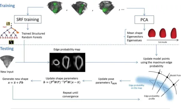
la distance absolue moyenne (MAD). Une série d’annotations est en RGB, et l’autre en MYC. L’image intitulée en rouge représente pour chaque paire d’annotations la variabilité moyenne sur l’endocarde. Première rangée : intra-variabilité. Trois dernières lignes : inter intra-variabilité. . . 25 1.6 Notre méthode SRF [31] . . . 29 1.7 Vue d’ensemble de notre pipeline complet combinant SRF et ASM pour la

segmentation du ventricule gauche en échocardiographie 3D. . . 30 1.8 Principales composantes de l’optimisation en apprentissage profond : a) Le

gradient à appliquer à W pour corriger l’erreur sur l’objectif est obtenu en appliquant le théorème de dérivation des fonctions composées à toutes les couches intermédiaires. Chaque poids est mis à jour d’une fraction de son gradient (taux d’apprentissage). b) Progressivement, le modèle converge vers un minimum local de la fonction de coût calculée sur l’ensemble des données d’entraînement. . . 33 1.9 Anatomical outliers from U-Net 2: a) is also a geometrical outlier but not b).

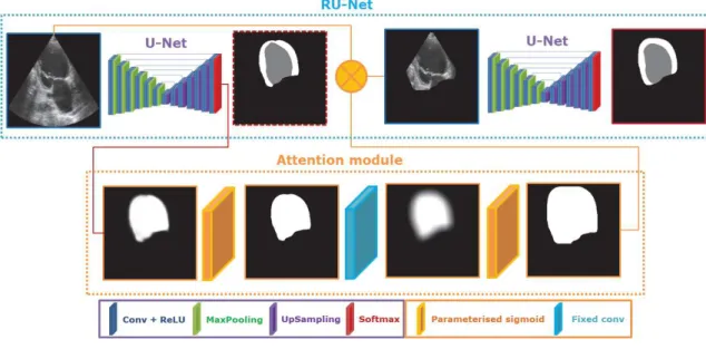
Local shape irregularities are cercled in yellow. . . 40 1.10 Illustration du modèle RU-Net. Les deux U-Nets sont indépendants

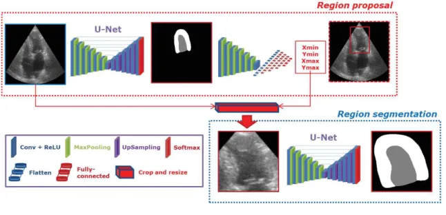
(paramètres séparés). . . 42 1.11 Illustration du modèle LU-Net avec le réseau de proposition de région

U-Loc2-multi-région, décrit dans la section 9.5.1. Les deux U-Nets sont indépendants. 43 3.1 a: 2D cardiac ultrasound probe (GE M5S). b: The emission / c: reception are

performed using piezoelectric materials [54]. . . 55 3.2 Longitudinal wave at a given time. As the wave propagates, particles oscillate

between a compression or rarefaction state [8]. . . 56 3.3 Interactions of the sound wave with soft tissues. Left: scattering eﬀect. Right:

Reﬂection, refraction, and attenuation [57]. . . 57 3.4 Focused beam onto a focal point. a: Each element receives a diﬀerent delay

according to the distance to the point. b: The same delays are applied on the received echoes before summation to create the radiofrequence (RF) echo signal [58]. . . 58

(23)

3.5 2D Long axis (LAX) view of the heart. The triangular sector clearly apparent in the B-mode image is decomposed into several lines. . . 59 3.6 Common artifacts in echocardiography (B-mode images). . . 60 3.7 B-mode and M-mode images. . . 61 3.8 Example of mitral regurgitation observed with color ﬂow Doppler imaging. . 62 3.9 Cardiac structures (a) and cycle (b). . . 63 3.10 Apical views used to estimates the ejection fraction with the Biplane Simpson

method, illustrated on Patient 206 of the CAMUS dataset (detailed in Chapter 5). . . 64 3.11 Monoplane Simpson decomposition of the heart’s volume from A4C views. If

we use the A2C, the disks are elliptic and better representative of the cavity [13]. . . 65 3.12 Cardiac function analysis through myocardial strain curves (on the right)

com-puted for each AHA segment (on the left). . . 65 4.1 Summary and comparison of the existing cardiac MRI datasets which were

released for challenges and are publicly available in 2017 [63]. . . 69 4.2 Cardiac segmentation in 3D ultrasound. . . 70 4.3 Multi-structure segmentation seen as a multi-label classiﬁcation problem.

Su-pervised learning algorithms are trained to predict b) from a). In visuals, we traditionally display the contours over the image as in c). . . 71 4.4 Illustrations from the active contour method in Chen et al. [76], with the

prediction in red and the ground truth in green. From a same initialization (a), enhancing the data-term (b) allows for a much better result than an enhanced shape constraint, which tends to shrink the LV (c). . . 74 4.5 Illustrations from the level-set approach from (Ning et al., 2002) [77]. First

rows: Multi-scale data-terms obtained by applying edge detection on the blurred downsampled image. Last row: Examples of segmentation results. . . 74 4.6 Illustrations of the deformable model from [81]. The groundtruth is in blue

while the proposed tracker’s prediction is in cyan and the comparative tracker in magenta. . . 75 4.7 Myocardium segmentation for strain estimation with speckle tracking [89]. . . 76 4.8 Visuals from the AAM of (Bosch et al., 2002) [93] on 3 frames of a single

se-quence. A: initialization, B: AAM position after 5 iterations, C: AAM position after 20 iterations, D: ground truth. . . 77 4.9 Edge maps from the SRF in (Domingos et al., 2014) [33]. The original slice is

on the left, the SRF prediction in the midle, and the reﬁned version using non maximum suppression on the right. . . 78 4.10 LV localization and segmentation from the deep learning approach in (Carneiro

et al., 2012) [18]. . . 79 4.11 Regularized CNN segmentation in 3D echocardiography [42]. . . 80 4.12 Average result from (Van Stralen et al., 2015) [102], color-coded in function of

the distance to the ground truth in orange. . . 81 5.1 Typical images extracted from the CAMUS dataset. The endocardium,

epi-cardium and left atrium wall are respectively shown in green, red and blue. (Left) input images, (Right) corresponding manual annotations. . . 92

(24)

5.2 CAMUS dataset samples to show the average expert variability with respect to the mean absolute distance (MAD). One set of annotations is in RGB, and the other in MYC. On the selected cases, the frame entitled in red depicts for each pair the average variability on the endocardium. First row: intra-variability. Last three rows: inter- variability. . . 93 6.1 Error maps of the method from Domingos and al. [16], compared to the second

best machine learning method and an expert.

The expert consensus is shown in grey. . . 95 6.2 Core elements of the RF algorithm: binary decision tree (a) allied to

random-izing strategies (such as b). Decision trees are a set of nodes routing the data to terminal nodes - called leaves - where the answer is stored. . . 96 6.3 Stump illustration and resulting information gain [62]. The stump function is

dotted. RFs perform linear cuts in the representation space. . . 97 6.4 Tree representation: The information stored at the leaves after the training

(here the histogram of labels) can be used at test time to assign a new class to the new data routed down to the leaf [108]. . . 98 6.5 (left) Street view, (middle) its corresponding segmentation masks, (right) the

prediction obtained from using RFs. [28]. . . 99 6.6 Ultrasound image of the heart and its corresponding segmentation

superim-posed. The drawn contours are smoothed though the image information shows no clear boundary. . . 100 6.7 Visualization of the nodes of a small tree (400 patches learnt). . . 104 6.8 Detection of the endocardium using default or tuned SRF (multi-scale features

+ larger patch size + all trees used at test time). . . 106 6.9 Relative number of calls for 7 scales of features on ten mid-size trees (5 × 104

patches). Regular features on the left, pairwise on the right. . . 106 6.10 Regular feature maps of a given image, the HOG arrows represent the direction

on which the gradient is projected . . . 107 6.11 Similarity feature maps of a given image. . . 108 6.12 Our SRF summary [31] . . . 111 6.14 Visuals for solved cases. Ground truth contours are dotted, while the algorithm

prediction is displayed in full line. . . 114 6.15 Visual for an unsolved case: Low contrast, unusual intensity patterns and

shape conﬁguration are in our opinion responsible. . . 114 6.16 3D volumes slices and the corresponding edge map slices from the apex to the

base. . . 116 6.17 Overview of our complete pipeline combining SRF and ASM for 3D

echocar-diography segmentation. . . 118 6.18 Correlation (left) and Bland Altman plots of all clinical indices. . . 120 6.19 Comparison between the prediction (yellow) and the groundtruth contours

(green) of the endocardium on both the B-mode image and the SRF edge probability map. . . 121 7.1 Generic CNN architecture [117] . . . 123 7.2 Auto-encoder architecture. . . 124 7.3 Example of cell segmentation with U-Net in microscopy images (DIC-HeLa

data set) [34]. . . 124 7.4 Representation of the layers and feature kernels of the U-Net [34] . . . 125

(25)

7.5 Visualization of the first layer filters learned by a reduced U-Net, and corre-sponding feature maps on a random validation image [122]. . . 127 7.6 Receptive fields [123]: After 2 3 × 3 convolutions, the pixel on the right contains

global information about the 5 × 5 region on the left. As CNNs get deeper, the receptive ﬁeld increases, allowing to extract high-level features. . . 127 7.7 Behavior of activated convolutions: while the convolution ﬁlters map values to

another representation, the activation sets saturation values. . . 128 7.8 Softmax output for the image in Fig. 7.5. Here the U-Net is used to segment

the LV (top right), the myocardium (bottom left) and the LA (bottom right). 129 7.9 Down and Up-sampling in CNNs examples. . . 129 7.10 Main components of the optimization in DL: a) The gradient to apply to W

to correct the error on the objective is obtained by applying the chain rule to all intermediary layers. Each weight is updated by a fraction of their gradient (learning rate). b) Progressively, the model converges to a local minima of the loss function computed on the training dataset. . . 130 7.11 Dropout illustration [130]. Left: base network, right: network with a dropout

rate around 40%. . . 132 7.12 Training curves of a reduced U-Net trained on 200 patients and validated

on 100 with a categorical cross-entropy loss and the Adam optimizer with a learning rate of 2 × 10−3_{. Dice results are given on the right. [122]. . . 133}

7.13 Average peformance representations. Left: U-Net, right: SRF. Top: 50 pa-tients, bottom: 400. "metric: LVendo | LVepi. . . 137 7.14 Evolution of the three geometrical metrics for an increasing training set size,

from 50 to 400 patients (i.e 200 to 1600 images). . . 138 7.15 Learning curve model [138]: y= (_{1 − a})_{− b × x}c _{with 0 < a ≪ 1 and c ∈}_[

−1, 0].139 7.16 Key components of the BEASM: an explicit formulation of contours

incorpo-rating shape constraints from an ASM. . . 143 7.17 Overlapping distributions of prediction results from U-Net 1 and U-Net 2. . . 148 7.18 Segmentation results obtained by U-Net 1 . . . 150 7.19 Segmentation results obtained by U-Net 2. . . 150 7.20 Segmentation results obtained by SRF. . . 151 7.21 Segmentation results obtained by the BEASM-f. . . 151 7.22 Segmentation results obtained by the BEASM-s. . . 152 7.23 Segmentation results obtained by O2. . . 152

7.24 Segmentation results obtained by O3. . . 153

7.25 Segmentation results obtained by O1b. . . 153

7.26 Segmentation results of U-Net 1 on Patient 252 (Medium IQ). . . 154 7.27 Anatomical outliers (up), one at ED only (down). . . 154 7.28 Bland Altman plots of the experts on fold 5 and of the algorithms on the full

dataset. . . 158 7.29 Tukey box plots of the geometrical results a) MAD; b) HD; c) Dice of the

U-Net 1 architecture for three diﬀerent schemes. . . 161 7.30 Evolution of the segmentation scores of U-Net 1 computed on fold 5 according

to the number of patients in the training dataset . . . 162 7.31 Geometric scores of the cardiologist-speciﬁc models. . . 163 8.1 Original architecture of U-Net++. Deep supervision in red shows that a same

loss L sends gradients to early reconstructions of the ﬁnal segmentation in X0,4_{. Additional convolutional layers on the skip connections are shown in}

(26)

8.2 Original architecture of SHG. The input of cascaded networks is the concate-nation of the original image and the previous segmentation result. . . 167 8.3 First two modes of an auto-encoder trained on fold 5 with a 94% average

accuracy, i.e. quantity of pixels rightly classiﬁed. Left: z=zmean− 4 × λp× vp, middle: z=zmean, right: z=zmean+4 × λp× vp. . . 169 8.4 Pipeline for segmentation tasks of the ACNN model, introduced in (Oktay et

al., 2017) [42]. . . 170 8.5 Segmentation results obtained by U-Net 1 ++. . . 173 8.6 Segmentation results obtained by SHG. . . 173 8.7 Segmentation results obtained by ACNN. . . 174 8.8 Bland Altman of the three EDNs on the full dataset. . . 175 8.9 Semantic amodal segmentation as introduced in (Zhu et al. 2017) [44].

In-stance segmentation masks are shown in the upper right, next to the image. Semantic masks are shown below the image next to corresponding contours. Finally, amodal contours are shown at the bottom, displaying continuity and simplicity to infer the hidden information. . . 177 8.10 Contours drawn by the two cardiologists of our study on the same case. Despite

the high distance between the annotations, the predicted shapes are similar in appearance. . . 178 8.11 Anatomical outliers from U-Net 2: a) is also a geometrical outlier but not b).

Local shape irregularities are cercled in yellow. . . 180 9.1 Mask R-CNN architecture of (He et al., 2017) [157]. A region proposal network

isolates regions of interest that two parallel branches classify and segment. . . 184 9.2 Pipeline and localization of lesion of (Pesce et al., 2019) [164]. . . 185 9.3 Illustration of the RU-Net pipeline. The two U-Nets are independent (diﬀerent

parameters). . . 187 9.4 Parameterized sigmoid with a slope=100and shift=0.5. . . 188 9.5 Illustration of the LU-Net pipeline with the U-Loc2-multi region proposal

net-work, described in Section 9.5.1. The two U-Nets are independent. . . 189 9.6 Attention-gated U-Net (a) and soft attention layer (b) introduced in (Oktay

et al., 2018). Attention layers are used in the upsampling branch to focus the skip connected features on regions of interest through the multiplication with attention maps built from the previous layer and the features to concatenate [47]. . . 192 9.7 Comparison of the segmentation performance of the baseline U-Net 1 (left

column) and the proposed LU-Net architecture (right column). In each image, the prediction is in green and purple while the ground-truth is in yellow and cyan. The BB estimated is displayed in red. . . 197 A.1 Collaborators from the Creatis laboratory: myself (left), my supervisors

(cen-ter), and the research engineer for the CAMUS platform (right). . . 209 A.2 Pierre-Marc Jodoin

- co-supervisor . . . 210 A.3 Collaborators from NTNU on the CAMUS study and attention-learning study:

scientiﬁc researchers (left) and clinical cardiologists (right). . . 210 A.4 Florian Espinosa

- cardiologist . . . 211 A.5 Collaborators from KU Leuven on the CAMUS study. . . 212 A.6 Collaborators from Erasmus MC on the SRF study. . . 212

(27)

C.1 Saki, indicated with the red arrow. . . 217 D.1 Camus dataset samples to show EF and IQ variability. First three rows: IQ

= G(ood), EF < 45, [45, 55], > 55. Last three rows: EF > 55, IQ = G(ood), M(edium), P(oor). . . 220 D.2 Leaderboard with the methods from [5] . . . 221 F.1 Reconstruction examples from the auto-encoders of our study. Left: ground

truth; Right: reconstruction. The ﬁrst two rows illustrate the average accuracy on the full CAMUS dataset. The last row shows an anatomically implausible reconstruction. . . 226 F.2 Geometric performance of ACNNs illustrated by standard error bars around

the mean values for the 5 segmentation networks. . . 228 G.1 Illustration of the reﬁnement in place in RU-Net. The ROI is shown in blue.

The ground truth is shown in yellow and cyan while the prediction is on green and red/magenta. On the U-Net epicardium contour (magenta), we see the epicardium being locally discontinuous while it is not the case for RU-Net (red).230

(28)

List of Tables

1.1 Étiquettes identiﬁant les structures cardiaques dans ce projet . . . 17 1.2 Caractérisation des diﬀérents types de méthodes de segmentation en

échocar-diographie, inspirée de la revue par (Carneiro et al., 2012) [18] . . . 18 1.3 Principales caractéristiques de la base de données CAMUS (500 patients) . . 22 1.4 Scores géométriques en ﬁn diastole . . . 31 1.5 Scores géométriques en ﬁn systole . . . 31 1.6 Précision de segmentation des méthodes évaluées sur les dix plis de CAMUS,

restreinte aux patients ayant une bonne & moyenne qualité d’image. . . 35 1.7 Paramètres cliniques des méthodes évaluées sur les dix plis de CAMUS,

re-streinte aux patients ayant une bonne & moyenne qualité d’image. . . 35 1.8 Critère d’aberrance anatomique . . . 39 1.9 Scores géométriques des 4 méthodes évaluées sur les patients de bonne et

moyenne qualité d’image (406 au total). . . 44 3.1 Speed of sound in common media . . . 56 4.1 Labels associated to identify cardiac structures in this project . . . 72 4.2 Characteristics of segmentation methods in echocardiography,

inspired from the review of (Carneiro et al., 2012) [18] . . . 72 4.3 Segmentation scores for the 14 evaluated methods on the test set of the

CE-TUS dataset (30 patients). The inter-expert variability is given prior to fully-automatic methods, semi-fully-automatic methods, and algorithms proposed after the challenge. The best scores in 2014 are given in blue while current ones are shown in bold. . . 83 4.4 Accuracy on clinical indices of the 14 evaluated methods on the test set of the

CETUS dataset (30 patients). The inter-expert variability is given prior to fully-automatic methods, semi-automatic methods, and algorithms proposed after the challenge. The best scores in 2014 are given in blue, current ones in bold. . . 84 5.1 The main characteristics of the CAMUS dataset (500 patients) . . . 90 6.1 Diﬀerences between Kontschieder’s and Dollár’s approaches of the structured

random forests . . . 102 6.2 Main diﬀerences between Dollár and al.’s and our hyperparameters . . . 110 6.3 SRF VS AAM segmentation results at ED . . . 113 6.4 SRF VS AAM segmentation results at ES . . . 113 6.5 3D SRF main hyperparameters . . . 116 6.6 Segmentation distance scores for end-diastole . . . 119 6.7 Segmentation distance scores for end-systole . . . 119 6.8 Clinical indices scores for end-diastole and end-systole . . . 119 7.1 Original U-Net architecture (28M parameters) . . . 125

(29)

7.2 Diﬀerences between the original U-Net and our ﬁrst architecture. Unmentioned parameters are unchanged. . . 135 7.3 Comparison between U-Net and SRF Training size = 50 patients / 200 images 136 7.4 Comparison between U-Net and SRF Training size = 400 patients / 1600 images136 7.5 Geometrical outliers criteria . . . 140 7.6 Main characteristics of U-Net 1 and U-Net 2 . . . 142 7.7 Segmentation accuracy of the 5 evaluated methods on the ten test folds,

re-stricted to patients having good & medium image quality (406 patients in total). . . 146 7.8 Outliers rates . . . 147 7.9 Segmentation accuracy of the 5 evaluated methods on fold 5 restricted to good

& medium image quality (40 patients). . . 149 7.10 Segmentation accuracy of the 5 evaluated methods on the ten test datasets

restricted to patients having poor image quality (94 patients). . . 149 7.11 Clinical metrics of the 5 evaluated methods on the ten test folds restricted to

patients having good & medium image quality (406 patients). . . 156 7.12 Clinical metrics of the 5 evaluated methods on fold 5 restricted to patients

having good & medium image quality (40 patients in total) . . . 157 7.13 Segmentation accuracy from U-Net 1 to U-Net 2. Bold values indicate a

su-perior value to U-Net 1. . . 159 8.1 Segmentation accuracy of U-Net++ for diﬀerent implementations, on the ten

test sets restricted to patients having good or medium image quality (406 patients) . . . 166 8.2 Segmentation accuracy of the 4 methods on the ten test folds, restricted to

patients having good & medium image quality (406 patients). . . 172 8.3 Geometrical outlier rates . . . 172 8.4 Clinical metrics of the 4 evaluated methods on the ten test folds restricted to

patients having good & medium image quality (406 patients). . . 175 8.5 Simplicity and convexity values computed from the three experts’ annotations

on 50 patients (200 images). Values in red correspond to the minimal value used for the outlier criteria. . . 178 8.6 Anatomical outlier criteria . . . 179 8.7 Anatomic scores and outlier rates computed on the full dataset (500 patients).

ana: anatomical , geo: geometrical . . . 180 9.1 Segmentation accuracy of U-Net 1 for a perfect prior localization of the

endo-cardial region, restricted to patients having good and medium image quality (406 in total). m indicates the margin value. . . 186 9.2 Localization accuracy on 4 evaluated methods on the full dataset (500

pa-tients). The m information contained in each method name indicates the margin value deﬁned in Section 9.3.2.1 . . . 194 9.3 Segmentation accuracy on the 4 evaluated methods restricted to patients

hav-ing good and medium image quality (406 in total). . . 195 9.4 Clinical metrics of the 4 evaluated methods restricted to patients having good

and medium image quality (406 in total) . . . 196 9.5 Segmentation accuracy and outliers on the full dataset (500 patients) including

those with poor image quality . . . 198 D.1 Population traits of the dataset . . . 219

(30)

E.1 U-Net 1 Architecture . . . 223 E.2 U-Net 2 Architecture . . . 224 F.1 Auto-encoder Architecture . . . 225 F.2 Segmentation accuracy for ACNN architecture with diﬀerent shape

regulariza-tion strengths . . . 227 G.1 Reﬁnement eﬀect on RU-Net with dil= 30 and shift= 0.7 Cross validation

on 10 subfolds of 200 images . . . 229 G.2 Geometrical performance and outliers for RU-Net : dil =11, shif t=0.5Cross

(31)

(32)

List of Abbreviations

Chapter 2

SVM Support Vector Machine RF Random Forest(s)

CAMUS Cardiac Acquisitions for Multi-structure Ultrasound Segmentation

Chapter 3

SNR Signal to Noise Ratio LV Left Ventricle RV Right Ventricle RA Right Atrium LA Left Atrium ED End Diastole ES End Systole

LV_EDV Left Ventricle End Diastole Volume LV_ESV Left Ventricle End Systole Volume EF Left Ventricle Ejection Fraction LV_EF Ejection Fraction

A4CH Apical 4 Chamber View A2CH Apical 2 Chamber View

Chapter 4 TP True Positive FP False Positive TN True Negative FN False Negative D Dice

JAC Jaccard index

MAD Mean Absolute Distance HD Hausdorﬀ Distance

MRI Magnetic Resonance Imaging CT Computed Tomography

CNN Convolutional Neural Network

ACDC Automated Cardiac Diagnosis Challenge

CETUS Challenge on Endocardial Three-dimensional Ultrasound Segmentation ASM Active Shape Model

AAM Active Appearance Model

BEAS(M) B-spline Explicit Active Surface (Model) SRF Structured Random Forest

(33)

DL Deep Learning

CNN Convolutional Neural Network

ACNN Anatomically Constrained Neural Network corr correlation

LOA Limit Of Agreement

Chapter5

IQ Image Quality

LV_endo Left Ventricle Endocardium LV_epi Left Ventricle Epicardium O₁ Observer 1

O₂ Observer 2 O₃ Observer 3

Chapter6

PCA Principal Component Analysis HOG Histogram Of Gradients LAX Long AXis view

Chapter7

CPU Central Processing Unit GPU Graphics Processing Unit EDN Encoder Decoder Network

Chapter8

DS Deep Supervision SHG Stacked HourGlasses

Chapter9

BB Bounding Box ROI Region Of Interest RU-Net Reﬁning U-Net LU-Net Localization U-Net

(34)

À Ginette et Jacqueline, mes grands-mères adorées,

To Ginette and Jacqueline, my beloved grandmothers,

(35)

(36)

Part I

(37)

(38)

Chapter 1

Résumé en Français (French

Summary)

L’étude présentée dans ce manuscript porte sur l’Automatisation de la segmentation

sémantique de structures cardiaques en imagerie ultrasonore par apprentissage supervisé. Ce premier chapitre est dédié à la reprise en français des points clés abordés

dans le manuscript complet écrit en anglais. À ce titre, il contient dans cet ordre :

• un abstract, synthétisant en quelques mots la thématique et les contributions; • une traduction du Chapitre d’introduction (2);

• une sélection du Chapitre présentant l’échocardiographie (3);

• une sélection du Chapitre sur l’état de l’art de la segmentation en échocardiographie (4);

• un résumé du Chapitre décrivant la base de données construite pour le projet (5); • un résumé du Chapitre sur l’adaptation de la méthode des forêts aléatoires structurées

pour la segmentation d’images échocardiographiques (6);

• un résumé du Chapitre sur l’évaluation du potentiel des méthodes d’apprentissage pro-fond pour la segmentation automatique d’images échocardiographiques (7);

• un résumé du Chapitre sur le perfectionnement des modèles d’apprentissage profond et de leurs métriques d’évaluation dans le cadre de la segmentation d’images échocardio-graphiques (8);

• un résumé du Chapitre sur l’amélioration de la robustesse de la segmentation produite par des modèles d’apprentissage profond grâce à l’ajout de mécanismes d’attention, appliqué à la segmentation d’images échocardiographiques (9);

(39)

1.1 Abstract

L’analyse d’images médicales joue un rôle essentiel en cardiologie pour la réalisation du diag-nostique cardiaque clinique et le suivi de l’état du patient. Parmis les modalités d’imagerie utilisées, l’imagerie par ultrasons, temps réelle, moins coûteuse et portable au chevet du pa-tient, est de nos jours la plus courante.

Malheureusement, l’étape nécessaire de segmentation sémantique (soit l’identification et la délimitation précise) des structures cardiaques est difficile en échocardiographie à cause de la faible qualité des images ultrasonores, caractérisées en particulier par l’absence d’interfaces nettes entre les différents tissus.

Pour combler le manque d’information, les méthodes les plus performante, avant ces travaux, reposaient sur l’intégration d’informations a priori sur la forme ou le mouvement du cœur, ce qui en échange réduisait leur adaptabilité au cas par cas. De plus, de telles approches nécessitent pour être efficaces l’identification manuelle de plusieurs repères dans l’image, ce qui rend le processus de segmentation difficilement reproductible.

Dans cette thèse, nous proposons plusieurs algorithmes originaux et entièrement automatiques pour la segmentation sémantique d’images échocardiographiques. Ces méthodes génériques sont adaptées à la segmentation échocardiographique par apprentissage supervisé, c’est-à-dire que la résolution du problème est construite automatiquement à partir de données pré-analysées par des cardiologues entraînés.

Grâce au développement d’une base de données et d’une plateforme d’évaluation dédiées au projet, nous montrons le fort potentiel clinique des méthodes automatiques d’apprentissage supervisé, et en particulier d’apprentissage profond, ainsi que la possibilité d’améliorer leur robustesse en intégrant une étape de détection automatique des régions d’intérêt dans l’image.

(40)

1.2 Introduction

Ce chapitre expose les motivations de ce travail, et les objectifs correspondants. Nous y présentons ensuite la méthodologie appliquée tout au long de la thèse et terminons par l’organisation du manuscrit.

1.2.1 Motivation

Le contexte scientifique dans lequel la présente étude a été menée comprend d’une part des défis cliniques et d’autre part des défis méthodologiques. L’identification de ces barrières nous a incité à définir des objectifs clairs pour chacun de ces aspects, et à élaborer des stratégies spécifiques pour les atteindre.

1.2.1.1 Contexte scientifique

Contexte clinique Les maladies cardiovasculaires ﬁgurent parmi les principales causes de

mortalité et de morbidité dans le monde. Alors qu’elles représentaient 30 % du total des décès en 2008, le nombre de victimes ne cesse d’augmenter, en partie à cause du vieillissement de la population. D’ici 2030, on estime que plus de 20 millions de personnes mourront chaque année des suites de telles maladies, ce qui encourage le développement de nouvelles pratiques en clinique afin de favoriser leur diagnostic précoce [2]. Comme la plupart des pathologies cardiaques affectent la forme et le comportement des structures cardiaques, l’imagerie médi-cale non invasive est une solution de choix car elle permet d’établir le diagnostic à partir de la visualisation des différentes structures cardiaques et de l’évaluation de leur fonctionnement. L’ imagerie par ultrasons est actuellement la modalité la plus utilisée pour l’imagerie car-diaque [3], car elle permet une bonne résolution temporelle à un coût relativement faible comparé aux autres modalités. Puisque l’usage de l’échocardiographie 3D est encore nouveau en routine clinique [4], l’imagerie ultrasonore 2D reste la modalité la plus répandue pour réaliser l’estimation d’indices cliniques tels que les volumes ventriculaires et les fractions d’éjection. Ces mesures reposent alors sur l’approximation de volumes à partir de surfaces, et dépendent fortement du processus d’acquisition.

En échocardiographie, le tissu myocardique apparaît dans l’image en forte intensité (blanc) et peut être différencié des cavités remplies de sang qui sont elles associées à des intensités basses (noir). La séparation et l’identification des différentes structures à partir d’une délim-itation précise, tâche d’analyse appelée segmentation sémantique, est la première étape pour effectuer des mesures de surfaces et de volumes.

Cependant, la segmentation en échocardiographie est une tâche particulièrement diﬃcile en raison de l’absence de frontières nettes, du faible rapport signal/bruit et de la texture chatoy-ante propre aux images échographiques appelée speckle, auxquels s’ajoutent de nombreux et complexes artéfacts d’image. La conséquence directe de ces attributs est que les logiciels réal-isant de manière entièrement automatique la segmentation d’images échocardiographiques fonctionnent assez mal, ce qui oblige les cliniciens à tracer les diﬀérents contours à l’aide d’outils semi-automatiques [5].

Contexte algorithmique Les annotations réalisées manuellement ou semi-automatiquement

ne sont pas reproductibles et sont sujettes, en plus d’être coûteuses en terme de temps, à des diﬀérences inter- et intra- observateurs. Aﬁn d’améliorer le déroulement de l’analyse car-diaque en routine clinique, l’automatisation de la segmentation du cœur a donc fait l’objet

(41)

d’intenses recherches au cours des dernières décennies, avec un eﬀort particulier sur la seg-mentation du ventricule gauche [3].

La segmentation en échocardiographie a été historiquement abordée par des méthodes de traitement d’image morphomathématique reposant sur lexploitation d’information pixellique et donc uniquement locale, puis par des algorithmes à base de contour actifs exploitant des contraintes pré-établies pour régulariser globalement les résultats de segmentation. En particulier, l’utilisation d’informations a priori sur la forme recherchée s’est avérée partic-ulièrement eﬃcace pour inférer à partir du contexte les interfaces localement manquantes dans l’image. D’autre part, l’incorporation de lissage temporel des résultats de segmentation a permis d’encourager une cohérence de la segmentation au long du cycle cardiaque.

Les méthodes d’apprentissage supervisé rassemblent des algorithmes eﬀectuant un mappage entre l’espace image et l’espace de solution dont les paramètres sont déduits de cas résolus (paires image/solution). Ces méthodes sont devenues populaires en vision par ordinateur au cours des années 90 grâce au développement des modèles de forme actifs [6], des machines à vecteurs de support (SVM) et des forêts aléatoires (RF) [7]. Cependant, la diﬃcultés d’obtenir des données annotées par des experts a limité leur application en imagerie médicale, et en particulier en échocardiographie.

1.2.1.2 Verrous techniques

L’établissement d’ensembles de données adaptés Le premier verrou technique pour

l’automatisation de la segmentation échocardiographique concerne le développement de larges ensembles de données annotées. Ces ensembles de données sont non seulement nécessaires pour l’entraînement des méthodes d’apprentissage supervisé, mais aussi pour l’évaluation précise de la performance des algorithmes.

Aﬁn de répondre aux besoins cliniques, un ensemble de données annotées de segmentation en imagerie médicale doit contenir et être représentatif de la variabilité à laquelle les cliniciens sont confrontés dans leur pratique quotidienne (pathologies, qualités d’image, matériels et paramètres d’acquisition...), c’est-à-dire ne pas être limité à des simulations, même réalistes, ou comporter uniquement des cas réels avec une qualité d’image élevée [3].

De plus, les annotations doivent être établies par des experts pour toutes les vues et tous les instants pertinents suivant un protocole fixé et consensuel, ce idéalement dans un contexte favorisant la précision (hors exercice et avec un logiciel de traçage approprié). Les mêmes structures d’intérêt doivent être annotées sur toutes les images, et tous les renseignements cliniques pertinents pour le patient doivent être renseignés avec les images de l’examen. Enfin, pour être entièrement validé et bénéfique pour la communauté, un tel ensemble de données devrait être publique d’accès, tout du moins aux chercheurs et aux cliniciens.

La construction d’algorithmes robustes et entièrement automatiques Le second

défi technique consiste à mettre en place des algorithmes de segmentation robustes et entière-ment automatiques comme socles de logiciels d’analyse fiables, assistant les cardiologues lors des examens (analyse d’image, calcul d’indices cliniques, guide d’acquisition...). En vue d’un diagnostic précis et reproductible, la robustesse des algorithmes devient l’un des principaux critères de qualité, en tant que mesure de fiabilité.

(42)

Afin d’encourager leur adoption en pratique clinique [3], la comparaison des méthodes doit être effectuée sur un ensemble de données large et validé, ce qui permet en plus de sélection-ner les meilleurs algorithmes de mieux analyser les limites des différentes approches. En ce qui concerne les méthodes d’apprentissage supervisé, l’analyse des erreurs réalisées par de multiples algorithmes sur un ensemble de données validé par la communauté peut également aider à évaluer les cas manquants dans la base pour une meilleure robustesse des modèles d’apprentissage.

Enﬁn, les solutions développées devraient idéalement être optimisées sur le plan de la vitesse dans le but d’être intégrées dans des logiciels d’analyse temps réel qui seront embarqués dans de nouvelles générations d’échographes.

1.2.2 Méthodologie 1.2.2.1 Objectifs

En raison de l’absence d’ensembles de données appropriés, la performance réelle des méth-odes de l’état de l’art en analyse d’images échocardiographiques n’est pas établie. Aﬁn de contribuer au développement d’une solution de segmentation automatique des structures cardiaques en imagerie ultrasonore qui soit adaptée aux besoins cliniques, ce travail a pour objectif d’apporter des réponses aux questions suivantes :

1. Quel est le potentiel des méthodes de segmentation sémantique par apprentissage su-pervisé en échocardiographie 2D ?

2. Sommes-nous proches d’une complète automatisation de l’analyse cardiaque en imagerie ultrasonore ?

1.2.2.2 Méthode

L’évaluation complète du potentiel des méthodes d’apprentissage supervisé pour l’analyse d’images échocardiographiques ne peut être eﬀectuée que par un étalonnage des méthodes les plus performantes sur un même ensemble de données. Cela nécessite :

1. d’utiliser un large ensemble de données annotées ;

2. d’établir un ensemble approprié de métriques géométriques et cliniques ;

3. de mettre en œuvre et d’adapter les techniques de l’état de l’art à notre problèmatique; 4. d’évaluer les méthodes sur une même plate-forme d’évaluation.

Ainsi, le potentiel clinique des algorithmes de segmentation automatique pourrait être établi à partir de :

1. la comparaison entre la meilleure méthode et les scores inter- et intra-experts ; 2. l’analyse des cas aberrants pour évaluer la robustesse ;

3. l’analyse d’erreurs aﬁn d’établir des pistes d’amélioration prometteuses;

4. l’élaboration de nouvelles méthodes dédiées à l’amélioration de la robustesse et de la précision de la segmentation.

La rigueur et la qualité de l’évaluation ont été notre principale priorité, ce qui nous a amenés à contribuer non seulement sur les aspects algorithmiques de la thématique, mais aussi sur les métriques utilisées pour mesurer la qualité du résultat.

(43)

1.2.3 Organisation du manuscript

Le manuscrit est découpé en quatre parties principales, toutes composées de chapitres in-dépendants qui abordent progressivement les aspects méthodologiques suivants :

1. Présentation

• Chapitre 1 : le résumé de la thèse, en français à la demande de l’école doctorale EEA, qui couvre toutes les discussions abordées dans le manuscrit en se concen-trant sur les points clés ;

• Chapitre 2 : l’introduction, dans laquelle les motivations et la stratégie méthodologique de la thèse sont présentées, ainsi que l’organisation détaillée du manuscrit.

2. Contexte

• Chapitre 3 : les bases de l’échocardiographie, où nous décrivons les aspects les plus pertinents de l’imagerie échographique cardiaque par rapport à cette étude; • Chapitre 4 : la revue de l’état de l’art, qui détaille les ensembles de données,

méthodes et métriques éxistants en segmentation d’images échocardiographiques. 3. Contributions

• Chapitre 5 : la création de la base de données CAMUS, à ce jour l’ensemble de données de référence libre d’accès le plus complet en échocardiographie 2D ; • Chapitre6: l’adaptation des forêts aléatoires structurées (méthode d’apprentissage

automatique) à la segmentation échocardiographique 2D et 3D;

• Chapitre7: l’étude et l’évaluation de méthodes d’apprentissage profond à travers l’architecture U-Net ;

• Chapitre8 : le perfectionnement des modèles encodeur-décodeurs et de leur éval-uation grâce à la conception de métriques anatomiques;

• Chapitre 9 : le développement de modèles intégrant des mécanismes d’attention, destinés à améliorer la robustesse de la segmentation.

4. Epilogue

• Chapter 10 : la conclusion, avec un retour sur les principales réalisations et le détail des perspectives de nos travaux.

Le manuscrit est complété par une série d’annexes : A la présentation des collaborateurs de ce projet ; B la liste des publications ;

C la description des ordinateurs utilisés dans l’étude ; D des informations supplémentaires sur le Chapitre 5 ;

E des informations supplémentaires sur le Chapitre7 ; F des informations supplémentaires sur le Chapitre 8 ; G des informations supplémentaires sur le Chapitre 9 ;

Pour ﬁnir, toutes les références sont listées dans la section bibliographique qui clôt le manuscrit.