Airline fleet assignment with time windows

Airline Fleet Assignment with Time Windows

Brian Rexing

Submitted to the Department of Civil and Environmental Engineering in partial fulfillment of the requirements for the degree of

Master of Science in Transportation at the

MASSACHUSETTS INSTITUTE OF TECHNOLOGY June 1997

@Massachusetts Institute of Technology 1997. All rights reserved.

Author ... ... _{S. . .. . . .}

Department of Civil and Environmental Engineering May 9, 1997

Certified by.

Associate Professor of

Cynthia Barnhart Civil and Environmental Engineering Thesis Supervisor

Accepted by. ... ... Joseph M. Sussman Chairman, Departmental Committee on Graduate Students

JUN

2

4

1997

m

Airline Fleet Assignment with Time Windows

by Brian Rexing

Submitted to the Department of Civil and Environmental Engineering on May 9, 1997, in partial fulfillment of the

requirements for the degree of Master of Science in Transportation

Abstract

Current fleet assignment models allow no variability in the scheduled departure time of flights even though exploiting this variability can result in more flight connection opportunities and a more cost effective fleet assignment. We present a generalized model that exploits this variability, simultaneously assigning aircraft types to flights and scheduling flight departures.

We model this problem as a simple variant to current fleet assignment models, assigning a time window to each flight and then discretizing each window, allowing the model to select the departure time. As problem size can become formidable, much larger than current fleet assignment models, we develop two algorithmic ap-proaches for solving the model. Our direct solution approach is good for speed and simplicity, while our iterative technique minimizes memory usage.

Using data from a major U.S. airline. we show that our model can solve real, large-scale problems, and we evaluate the effects of schedule flexibility. In every test scenario, the model produces a fleet assignment with significantly lower costs than the basic model, and in a separate analysis, the model is used to tighten the schedule, potentially saving aircraft.

Thesis Supervisor: Cynthia Barnhart

Acknowledgments

I would first like to thank the people with whom I worked closely on this project, most notably Professor Cynthia Barnhart. Her guidance, motivation, and peanut M&Ms have made this project enjoyable and worthwhile. Thanks also to Tim Kniker for his OR insights and computer-related assistance. Of course, much thanks goes to United Airlines for funding this project and providing a source for understanding operational issues.

I'd like to thank the friends I've met as a part of the many athletic teams I've been on, particularly the club volleyballers, the Ashdown softball gang, and the Course 1 football team. These friends, and the competitive outlet they provided, always gave me something to look forward to during hectic weeks.

A special thanks to my best friends in Boston. I could not have asked for more from an officemate than Paul Carlson. The academic and career tips he's given me, as well as his model of discipline, will not be forgotten. Thanks to Bridgit Green for making my last six months in Boston the best of my short stay.

Finally, I'd like to thank the most important people in my life-my family. I've been able to learn from the intelligence of my father, the energy of my mother, and the guts of my brother.

Contents

2.1.1 Network Representation . ... .. 15

2.1.2 Formulation ... ... 16

2.2 Fleet Assignment with Time Windows Model . ... 20

2.2.1 Network Representation ... .. 20

2.2.2 Formulation ... ... 21

3 Solution Approach 24 3.1 Network Preprocessing ... ... 24

3.1.1 Node Consolidation ... .... 25

3.1.2 Deleting Redundant Arcs . ... . 25

3.1.3 Islands ... ... 26

3.2 Iterative Solution Technique (IST) . ... 28

3.2.1 The IST Algorithm ... ... 29

3.2.2 An Example ... ... 37

4 Computational Experiences 44

4.1 Implementation and Data ... ... 44

4.2 Preprocessing Results ... . ... ... . . . .. 46

4.3 Algorithm Performance .... .... ... ... . . 48

4.4 Solution Analysis . . . ... ... . 50

5 Conclusions and Future Research 54

List of Figures

2-1 A two-airport flight network . ... .... 16

2-2 Basic fleet assignment model ... ... 17

2-3 Time window flight network ... .... 20

2-4 Time line representation of a bank . ... 21

2-5 Fleet assignment with time windows model . ... 22

3-1 Deleting redundant flight copies ... .. 26

3-2 Time line with islands ... ... 27

3-3 Time window-expanded time line with islands ... .. .. . . . . 27

3-4 (a) Real-duration and (b) reduced-duration flight arcs ... . 30

3-5 Flowchart of the iterative solution technique (IST) . ... 31

3-6 Backward connection arcs ... ... 32

3-7 IST subproblem formulation ... ... 34

3-8 (a) Reduced-duration arc and (b) real-duration flight copies .... . 34

3-9 Basic flight network ... ... 38

3-10 Iteration 1, Master Problem network . ... 38

3-11 Iteration 1, Subproblem 1 network . ... 38

3-12 Iteration 1, Subproblem 2 network . ... 39

3-13 Iteration 2, Master Problem network . ... 39

3-14 Iteration 2, Subproblem 1 network . ... 40

3-15 Iteration 2, Subproblem 2 network . ... 40

3-16 Backward connection arcs ... ... 41 3-17 (a) Single reduced-duration arc and (b) three real-duration flight arcs 42

m

3-18 "Super master problem" flight network . ... 42

List of Tables

1.1 _{Flight connection example .}

Notation for the basic fleet assignment model . . . . Notation for the fleet assignment with time windows model

Notation for the IST subproblems ... Six-flight, two-fleet example . ...

Primary data sets . ...

Preprocessing reduces problem size . ...

Run times for DST and IST approaches (in minutes) . Problem sizes, measured in non-zero elements (at final IST) ...

P2-20.5 IST statistics . . . .

Solution improves as window width increases . . . . . Solution improvements for different copy intervals . . . Re-fleeting and re-timing statistics . . . .... Minimizing the number of aircraft utilized . . . .

17 22 iteration for . . . .. . 49 .. . . . . 50 . . . .. . 51 . . . . . 52 .. . . . . 53 53 2.1 2.2 3.1 3.2 4.1 4.2 4.3 4.4 4.5 4.6 4.7 4.8 4.9

Chapter 1

Introduction

1.1

Problem Description

Deciding when and where to offer flights is not the end of the airline schedule planning process. Given these initial strategic decisions, the schedule planner must resolve a series of issues before the schedule is actually operational. These issues include, among others, assigning aircraft to flight legs, routing the aircraft to ensure maintenance, and crew scheduling. The allocation of aircraft to flight legs, or fleet assignment, is the first of these issues that is addressed.

Fleet assignment has a tremendous impact on an airline's profits, as it directly affects flight operating costs and passenger revenues. Consider, for example, a large aircraft flying a leg with very few passengers, versus a small aircraft serving a route with high passenger demand. In the first case the prohibitive cost of flying the large aircraft was unnecessary, while in the second case the airline lost potential revenue, because passengers that would not fit on the aircraft were turned away. Clearly, an efficient fleet assignment depends on accurate forecasts of operating costs and passenger traffic. The traffic forecasts, together with known aircraft seating capacities and expected fares, allow the calculation of spill costs, or lost revenue due to under-capacity. With operating costs, spill costs, aircraft data, and schedule data now known, we can define the basic fleet assignment problem:

plus spill) according to each aircraft type on each flight leg, find the least cost assignment of aircraft types to flights, such that (1) each flight is covered by exactly one fleet type, (2) flow of aircraft by type is balanced at each airport, and (3) only the available number aircraft of each type are used.

Although not discussed in this paper, other constraints may be added to this prob-lem to improve the likelihood that the solution will be operational. These include considerations for gate and maintenance availability, crew scheduling, and aircraft noise.

This paper describes a daily fleet assignment problem, meaning we assume that the airline's schedule repeats day after day. This assumption is not too restrictive, as most U.S. domestic airlines fly the same schedule every day (with some exceptions), and demand among flights typically varies in the same direction and relative mag-nitude throughout the week. Some airlines deviate from this repeating schedule on weekends, but re-fleeting for these exceptions is handled after the daily assignments have been made.

Models that solve the basic daily fleet assignment problem have found wide acceptance among airlines, but despite their importance, these models leave room for improvement. One of the most noticeable weaknesses of current fleet assignment models is their requirement that flight departure times be fixed. In reality, the schedule used as an input to the fleet assignment model is not cast in stone; many of the scheduled times will be tweaked in the weeks leading up to the day of departure to improve such factors as gate availability and passenger connection times. It is also not uncommon for schedulers to manually re-time flights in search of an improved fleet assignment. The example in Table 1.1 illustrates how modifying the schedule may allow a better fleet assignment. Notice that both flights A and B have the same forecasted demand, and thus an assignment of the same type of aircraft to both flights might be appropriate. But, since flight A's ready time (arrival time plus minimum ground service time) is after flight B is scheduled to depart, the same aircraft cannot cover both flights. However, if flight B could be re-timed to depart

Departure Ready

Flight Origin Destination Time Time Demand

A BOS ORD 0800 1000 150

B ORD DEN 0955 1200 150

Table 1.1: Flight connection example

after 1000, the connection could be made, and a single aircraft could cover both flights, possibly improving the fleet assignment.

By adding time windows, which define by how much time any given flight can shift, the set of feasible fleet assignment solutions grows substantially, and the opti-mal solution is guaranteed to be at least as good as the basic (fixed departure time) model. So then, the fleet assignment with time windows problem is the same as the basic problem, except that time windows, rather than fixed departure times, are given for each flight.

1.2

Literature Review

Because of their effectiveness in improving profits, not to mention the efficiency of the planning process, airline schedule development models have been given much attention. This is evident in Gopalan and Talluri [8], a survey of mathematical models used during schedule development. Fleet assignment in particular is a well-researched topic, with Daskin and Panayotopoulos [6], Abara [1], Berge and Hop-perstad [3], Hane et al. [10], Subramanian et al. [12], Gu et al. [9], and Clarke et al. [4] each presenting formulations to variations of the basic daily fleet assignment model within the last eight years. Daskin and Panayotopoulos [6] present an inte-ger program that assigns aircraft to routes (which they define as sequences of flight legs originating and terminating at the same airport) in single-hub networks. La-grangian relaxation is used to find an upper bound, and heuristics are used to find specific solutions. Abara [1] presents a model that can be used for more general airline networks, but the model has some limitations due to the choice of "feasible turns" (connection arcs) as decision variables. The model size explodes unless

its are placed on the connection opportunities. Another limitation is that different flying times and turn times (minimum ground service times) are not allowed for different fleets. Berge and Hopperstad [3] present a "fundamentally new operating concept" for dynamically re-assigning aircraft as traffic forecasts change throughout the planning horizon. Since the re-assignment problems involve only a common-cockpit subset, or "family," of an airline's aircraft (so as not to destroy the crew assignments), the problems are smaller than an airline's full daily problem. These problems are formulated as multicommodity network flow problems on space-time networks. To obtain quick solutions, two heuristic algorithms specifically designed for these small re-assignment problems are suggested: one heuristic solves a sequence of single-commodity flow problems, and the other begins with a feasible assignment and performs multiple profit-improving aircraft swaps. Hane et al. [10] use a similar multicommoditv network flow formulation to solve the basic fleet assignment prob-lem, but their use of variable aggregation, cost perturbations, dual simplex with steepest-edge pricing, and intelligent branch-and-bound strategies result in a rapid solution to realistically-sized (2500-flight, eleven-fleet) problems. Gu et al. [9] study the complexity and behavior of the model presented in the Hane paper, while in Clarke et al. [4], a sequel to the Hane paper, it is shown that better operational solutions to the fleet assignment problem can be achieved by adding variables and constraints that model maintenance and crew issues.

Levin [11] was the first to propose a scheduling and fleet routing model with time windows, however this model did not consider multiple fleet types. Time windows were modeled by allowing departure times to occur at discrete intervals within the time window. Much more recently, Desaulniers et al. [7] presented two formulations to the fleet assignment and aircraft routing problem with time windows. These equivalent formulations are solved by decomposing the problem and generating fa-vorable flight paths with time-constrained shortest path subproblems. The models are demonstrated to be effective on small (less than 400 flights/day) examples.

In this paper we consider large scale problems of fleet assignment with time windows. The contributions of this paper include the following:

1. By discretizing each flight's departure time window, we model the fleet as-signment with time windows problem as a simple variant of the basic fleet assignment model. Ours is a generalized model and solution approach for fleet assignment, in that time windows of zero width can be used (resulting in the basic fleet assignment model) or flights can be given time windows of varying width. Furthermore, the structural similarity between our model and those models currently implemented at many airlines is a key attribute of our approach.

2. We present two algorithmic approaches for solving the fleet assignment with time windows model. Both approaches begin with network preprocessing, some of which we designed specifically for our new model. Then, we demon-strate that the model can be solved either directly or by using an iterative solution technique. Our direct solution approach (DST) is good for speed and simplicity, while our iterative approach (IST) minimizes memory usage (which is valuable for larger problems and problems with added enhancements). 3. Using data from a major U.S. airline, we show that our model can solve real,

large-scale problems, and we evaluate the effects of schedule flexibility. We take an in-depth look at the effects of network preprocessing, compare the performance of our two algorithms, and show that allowing time windows can save aircraft, as well as improve daily operating and spill costs. For example, on a 2037-flight, seven-fleet problem with time windows of a maximum of +/- _{10 minutes on all flights, our model finds a solution that reduces fleet} assignment costs by over $67,000 per day beyond the optimal solution with no time windows. In that solution, less than 6%, of all flights are moved from their originally scheduled time. In a separate analysis on the same problem instance, we find that the flight schedule can be flown with two fewer aircraft

than are necessary when departure times are fixed. Although the operational feasibility of these new solutions must be verified, the results are certainly promising.

1.4

Outline

In Chapter 2 we describe the mathematical model and flight networks for fleet as-signment with time windows. In Chapter 3 we detail the network preprocessing steps and then motivate and describe the alternative solution techniques we have designed. Chapter 4 presents results and computational experiences obtained in solving fleet assignment problems for a large airline. Finally, in Chapter 5 we sum-marize this research and suggest pertinent future research.

Chapter 2

Mathematical Model

In this chapter, we present the integer programming formulation to the fleet as-signment with time windows problem. Because the formulation used is a simple extension of the basic fleet assignment problem, we begin by describing this basic formulation.

2.1

Basic Fleet Assignment Model

2.1.1

Network Representation

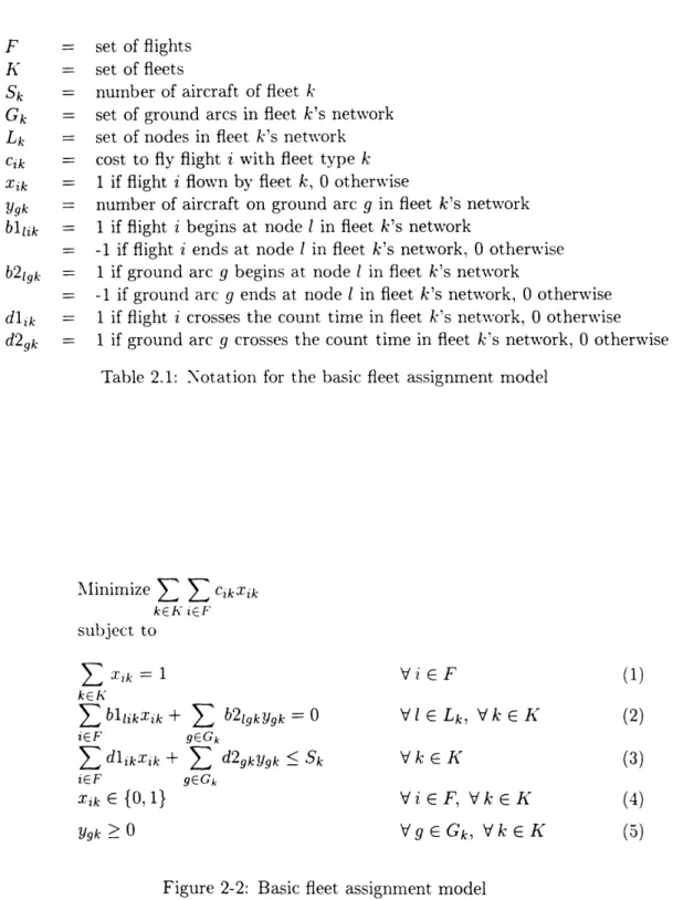
The flight networks are the foundation upon which the fleet assignment model is built, for they ensure feasible flight connections, conservation of aircraft flow, and a balanced number of aircraft of each type at each airport at the beginning and end of each day. A different flight network is created for each fleet type, and it is made up of parallel time lines-one time line for each airport. An example of a two-airport, four-flight network is shown in Figure 2-1. Each time line is comprised of a series of ground arcs that connect event nodes. Event nodes represent departures or arrivals at an airport at a specific time. The parallel time lines are connected by flight arcs, which are defined by their departure and arrival nodes. Wrap-around arcs, which are just special-case ground arcs, connect the last event node to the first event node at each airport. This guarantees flow balance.

BOS

ORD

Figure 2-1: A two-airport flight network

not actually placed at the flight's arrival time; rather they are placed at the flight's ready time. If we did not place arrival nodes at each flight's ready time, we might allow aircraft to connect to departing flights before they are actually prepared to leave. For example, in Figure 2-1, if flight B were put on the BOS time line at its arrival time. an aircraft would then be allowed to flow across both flight B and flight C. which is actually impossible. Turn times, which can be different for every fleet type. are typically 30 to 40 minutes for domestic flights, depending on aircraft size. Since we create a different network for each fleet type, we can model not only this disparity in turn times. but also the differences in flying times among different aircraft types.

2.1.2

Formulation

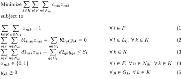
Once the flight networks have been built for each fleet, the basic fleet assignment problem can be solved using the formulation given in Figure 2-2. Notation for this formulation is given in Table 2.1. Stated simply, this formulation seeks to minimize the cost to cover each flight with one aircraft type (constraints 1), making sure aircraft flow is conserved at each node (constraints 2), while using no more aircraft of each type than are available (constraints 3). The third constraint set counts aircraft of each fleet type by summing the flow on all arcs of that fleet's network that cross an arbitrarily chosen count time. A typical count time is 3:30 AM, because

F = set of flights

K = set of fleets

Sk = number of aircraft of fleet k

Gk = set of ground arcs in fleet k's network Lk = set of nodes in fleet k's network Cik = cost to fly flight i with fleet type k

Xik = 1 if flight i flown by fleet k, 0 otherwise

Ygk = number of aircraft on ground arc g in fleet k's network bllik = 1 if flight i begins at node 1 in fleet k's network

= -1 if flight i ends at node I in fleet k's network, 0 otherwise b2lgk = 1 if ground arc g begins at node I in fleet k's network

= -1 if ground arc g ends at node I in fleet k's network, 0 otherwise dlik = 1 if flight i crosses the count time in fleet k's network, 0 otherwise

d2gk = 1 if ground arc g crosses the count time in fleet k's network, 0 otherwise Table 2.1: Notation for the basic fleet assignment model

Minimize E E CikXik kEK iEF subject to

E

1

Sbllikik

+

E

b2lgkYgk =

0

1:

dlikXik

+

1>

d2gkYgk

Sk

E

{0, 1}

K

Vk e K

only wrap-around arcs and a few (red-eye) flight arcs cross this time. Decision variables x define which fleet type covers each flight, so these variables must be

integer (constraints 4). The y variables are zero-cost ground arcs that are necessary to preserve conservation of flow and to count the number of aircraft used. These variables need not be defined as integer (constraints 5), as the integrality of the flight variables ensures integral ground flow.

Objective Function Coefficients

Determining accurate cost coefficients is easily the most important, and difficult, factor in obtaining an efficient fleet assignment solution. Each coefficient, as was described in Section 1.1, is comprised of two parts: an operating cost and a spill cost. The operating cost portion (fuel, maintenance, crew, etc.) is relatively easy to estimate, however it can become more complicated as passenger-related costs are added. Passenger-related costs are a function of the number of passengers carried, which is a function of aircraft size.

Given an unconstrained demand for a flight, in order to calculate the expected number of passengers carried on that flight for a given fleet type, we must calculate the expected spill. Recall that spill is the number of passengers turned away by an airline, because demand was greater than seating capacity. Before discussing the possible methods for calculating spill, we define the following expressions:

spillik = expected number of passengers spilled from flight i if flown by fleet k

Pi = mean unconstrained demand of flight i

ai = standard deviation of demand of flight i capk = seating capacity of fleet k

maxLFi = maximum load factor allowed on flight i (< 1)

fz(xo)

spillik = max{0, Pi - caPk} (2.1)

greater than capacity. However, unless demand is deterministic, equation (2.1) underestimates spill. Consider, for example, a flight that has a mean unconstrained demand of 100 passengers and an aircraft with a capacity of 100 seats. Equation (2.1) tells us that there is an expected spill of zero passengers. Assuming that the demand actually varies from day to day, this estimate is clearly wrong, for any time the demand exceeds 100, there will be spill.

A simple and artificial way to account for this stochasticity in demand is to place a limit on the effective capacity of an aircraft as follows:

spillik = max{O, pi - maxLFi * capk} (2.2)

Using the example from above with a maximum load factor of 0.9, our estimate of spill becomes 10 passengers.

However, the most realistic approach for calculating spill is to assume that de-mand has a normal distribution, and calculate spill accordingly, as discussed in Subramanian et al. [12] and shown in equation (2.3) below.

pidlik = fx(xo)(xo - capk)dxo (2.3)

Given our estimate of spill, we can determine a spill cost for each flight-fleet pair. Spill cost is the expected number of passengers spilled multiplied by spill fare-an estimate of the average revenue per spilled passenger on that leg. Spill fare is another piece of data (in addition to mean unconstrained demand and its standard deviation) that is difficult to estimate, yet has significant impact on the fleet assignment solution. In our implementation we have assumed spill fare to be equivalent to the average fare paid on that leg.

BOS

A B C "D

ORD

Figure 2-3: Time window flight network

2.2

Fleet Assignment with Time Windows Model

2.2.1

Network Representation

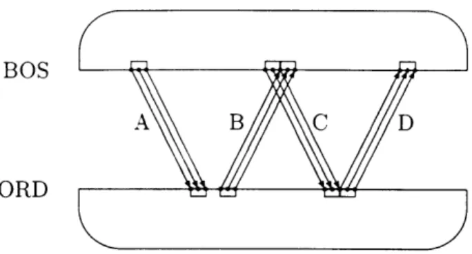
Time windows can be modeled with a simple, albeit computationally expensive, ex-tension of the basic flight networks. By placing copies of a flight arc at specified intervals within that flight's time window and requiring just one of the flight arc copies to be covered, we allow the model to choose the departure time of the flight. Figure 2-3 shows how the basic network of Figure 2-1 might look after being ex-panded to permit flexible departure times for each of the four flights. The departure and corresponding arrival time windows are indicated by the rectangles above (be-low) the BOS (ORD) time line. The impact that time windows have can be seen in this small example: a single aircraft may now cover flights B and C (by using the first copy of flight B and the last copy of flight C), whereas this connection was not possible in the basic model.

Because the scheduled time of some flights is more flexible than others, the width of each time window is a parameter that can be different for every flight. Obviously, wider time windows will allow more connections, but if a flight is moved too far from its originally scheduled time, then the passenger demand for that flight may change. Shuttle flights, arrival slot-controlled flights (e.g. at some international and congested domestic airports), and flights that are members of banks are examples of

FGH I J

HUB

ABCDE

Figure 2-4: Time line representation of a bank

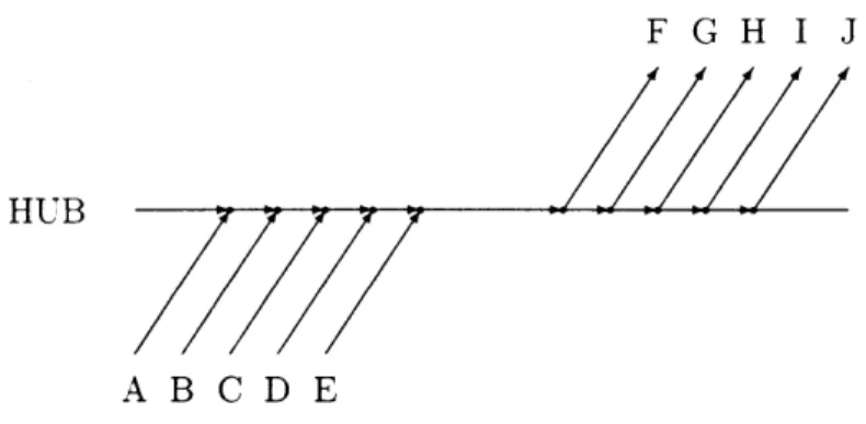
flights that may have a tightly constrained (possibly zero-width) time window. A bank is a hub airport activity that allows passengers from many origins to connect to flights that are departing to many different destinations. Figure 2-4 shows what a small bank would look like at the hub airport. So as not to clutter the figure, the basic network representation is shown (i.e. only one arc is shown for each flight). One can see why bank flights may have tightly constrained time windows by considering flight E. If flight E were allowed to arrive any later than its originally scheduled time, some passengers may not have time to run across the airport and board outbound flight F. So, flight E's time window may be, for example, [-10, 0] meaning it can be re-timed up to ten minutes earlier, but cannot be re-timed any later than its originally scheduled time.

The interval at which flight copies are placed within each time window is another parameter that can affect the quality of the solution. To guarantee that flights are allowed to depart at any time within their window, copies need to be placed at one-minute intervals. However, it will be shown in Sections 4.3 and 4.4 that using a narrow interval causes an explosion in the problem size, often without the benefit of providing a substantially better solution than a broader (say five-minute) interval.

2.2.2

Formulation

The fleet assignment with time windows model is almost exactly the same as the basic model, only it contains more variables and has slightly different coverage

Nik = number of arc copies of flight i in fleet k's network

Cnik = cost to fly copy n of flight i with fleet type k Xnik = 1 if copy n of flight i flown by fleet k, 0 otherwise

bllnik = 1 if copy n of flight i begins at node 1 in fleet k's network

= -1 if copy n of flight i ends at node 1 in fleet k's network = 0 otherwise

d1nik = 1 if copy n of flight i crosses the count time in fleet k's network = 0 otherwise

Table 2.2: Notation for the fleet assignment with time windows model

Minimize E E E CnikXnik

kE K icE F nE Nik

subject to

E Xnik 1

ViEF

(1)

kEK nENik

E

S

bllnikXnik +

5

b2lgkYgk =0

ELk, Vk

c

K

(2)

iEF nENik gEC;k

E

S

E

d2gkygk

Sk

V k E K

(3)

iEF nE lNik gEGk

Xnik {0, 1} Vi E F, Vn E Nk, V k E K (4)

Ygk > 0 Vg E Gk, V k E K (5)

Figure 2-5: Fleet assignment with time windows model

straints. Notation that is different from the basic model's notation is given in Table 2.2, and the new model is shown in Figure 2-5. This model is structured the same as the basic model, with the objective function minimizing cost, and the con-straints ensuring flight coverage (concon-straints 1), conservation of flow at each node (constraints 2), restricted aircraft utilization (constraints 3), and variable integrality (constraints 4, 5). Notice that there is still one constraint for every flight (1), node (2), and fleet type (3). However, there are far more nodes in the network when time windows are used. As explained in Section 2.2.1, constraints on a flight's time window width are modeled by only defining flights arcs that are within that flight's time window.

Notice in the first constraint set that only one arc, among all copies and every fleet, must be covered for each flight. By choosing a single arc copy, the model

effectively chooses the departure time of each flight. This model also allows the user to apply a different cost coefficient to every flight copy. So, for example, one can make it more expensive to fly a flight the further it is moved from its originally scheduled time.

Chapter 3

Solution Approach

The LP matrix of the fleet assignment with time windows model can become pro-hibitivelv large for realistically-sized problems. As such, preprocessing steps, de-scribed in Section 3.1, are useful for reducing the model's size. After preprocessing, it is often possible to solve the fleet assignment problem directly. However, the direct solution approach requires that we include many unnecessary flight arcs. An alternative strategy, described in Section 3.2, is to iteratively add necessary flight arc copies to the model., thereby minimizing the model's size. For illustration of the iterative algorithm solution procedure (Section 3.2.1), an example is detailed

(Section 3.2.2).

3.1

Network Preprocessing

Because of the cumbersome size of fleet assignment models, substantial efforts have been made to prune the problem before the LP matrix is constructed and solved. Hane et al. [10] provide an excellent description of techniques that can be used before solving the basic fleet assignment model. Some of the same concepts are also appropriate for the fleet assignment with time windows model-a model with many more nodes and arcs than the basic model. Described below are three techniques that we use to reduce the network size; specific results of the impact of these techniques is given in Section 4.2.

3.1.1

Node Consolidation

Node aggregation, or consolidation, is one of the techniques described in Hane et al. [10] that can also be applied to networks with flight copies. The idea here is to replace one or more arrival nodes that are followed by one or more departure departure nodes, with a single node. For example, in Figure 2-4 all ten nodes and the nine ground arcs between them can be replaced by a single node without introducing illegal connections. Rather than representing a specific instant in time, this single node now represents a time range: from the ready time of flight A to the departure time of flight J. If flight H were an arrival, then flights A-G would be consolidated followed by a ground arc into a single node for flights H-J. Each node (ground arc) removed translates into exactly one less row (column) in the LP matrix.

3.1.2

Deleting Redundant Arcs

This is a technique that is unique to networks containing copies of individual arcs (such as our time window flight networks). After nodes of the flight networks have been consolidated, a set of redundant arcs can be defined as arcs of the same flight that have the same cost and share the same tail node. Among these redundant arcs, the first (earliest on the time line) copy dominates the later copies, because an aircraft flowing across the first arc can make, at a minimum, the same connections

as any of the later-arriving flights.

Figure 3-1 shows a portion of a flight network, after node consolidation, contain-ing a scontain-ingle flight with five arc copies between CMH and ORD. In this example there are two sets of redundant copies: (1,2) and (3,4,5). Assuming these arcs all have the same cost, arcs 2, 4, and 5 can be deleted from the network without affecting the solution. That is, the flights arriving at CMH and the flights departing from ORD have the same connection opportunities with or without these dominated arcs. However, if costs among copies of a flight are not the same, then arcs within a redun-dant set can only be deleted if they have both a later departure time and a cost not less than another earlier arc within that set. In any case, each arc deleted equates

ORD

CMH

Figure 3-1: Deleting redundant flight copies

to three fewer variables and two fewer constraints in the model (before node consol-idation). Not only is a flight arc (and its two end nodes) removed, but a ground arc is implicitly removed from each airport's time line as two arcs are merged into one.

VWe should note that in our implementation, one arc copy is always placed at the originally scheduled departure time of each flight, and this arc is never deleted. To further favor flights that depart at the originally scheduled time, we reduce the cost of these arcs by a very small amount.

3.1.3

Islands

Another of the techniques presented by Hane et al. [10] is to remove ground arcs from sparsely-used airports when it is known that no aircraft will be on the ground at that time. Removing these ground arcs leaves the time line with islands-periods of time when there is at least one aircraft on the ground. Figure 3-2 is an example of what a time line with islands might look like for the basic fleet assignment problem (one arc for each flight). By counting the arrival flights and departure flights, we can identify the maximum number of aircraft that might use each ground arc. For example, here we see that if there are x aircraft on the ground in the morning, then there must be x - 1 aircraft on the ground after the first departure. We continue down the time line, adding to the count for each arrival and subtracting from the count for each departure. The ground arc(s) with the lowest count can be removed. In this example, x- 1 is the lowest count, and so the two ground arcs with that count

B

Figure 3-2: Time line with islands_A

Figure 3-2: Time line with islands

Figure 3-3: Time window-expanded time line with islands

are removed. In this case the wrap-around arc is the only ground arc that might have aircraft flow. Notice that removing ground arcs not only removes variables from the problem. but in some cases it also fixes the connections between flights. In this case, if the model chooses the fleet of this time line to cover flight A, then it must also cover flight B.

Figure 3-3 shows what Figure 3-2 might look like after flight copies are added to model time windows. As one can see, there may be a different number of copies for each flight due to differences in time window width and the effect of deleting redundant copies of that flight. This example shows that the process of counting arrival and departure arcs to identify islands becomes more difficult when there are multiple copies of each flight. When counting arrivals and departures, one must only count the last copy of each flight. Ground arcs that sit between the first and last copies of flights should be given the same aircraft count as the previous ground arc. This means that in Figure 3-3, the small ground arc between copies of flights A and B gets a count of x - 1. Once again, it is found that the wrap-around arc is the only ground arc which may have aircraft flow.

As mentioned previously, this technique should only be applied on time lines z.A- -1 z .. Figure 3-2: Time line with islands m

of little activity, for it is on these time lines that the assumptions of the counting technique are most likely to be true. To guarantee that we are not eliminating arcs that may be in the optimal solution, the counting technique described requires that arrival flights connect to departure flights emanating from the same node. At heavily used airports it is less likely that this is true; here it is best that we leave the ground arcs and let the model choose the connections.

3.2

Iterative Solution Technique (IST)

After creating the flight networks and preprocessing, one option for solving the fleet assignment with time windows problem is to input the entire LP matrix into an LP solver and solve the problem directly. Advantages of a direct solution technique (DST) include simplicity and quickness in solving most problems. However, despite the gains made in preprocessing, DST has a disadvantage of including many un-necessary flight arc copies. That is, there are many flight arcs that are not deleted during the preprocessing phase that are unnecessary for achieving good solutions. Stated another way, even if many of the flight's departure times are fixed (i.e. only a subset of all flights are given time windows), the model can still achieve the same optimal solution as it does when all flights have time windows. The difficulty lies in identifying which flights need time windows and which flights can be fixed. The IST algorithm, described in the following section, does just that.

The iterative approach is to first solve a fleet assignment problem with one arc for each flight-fleet pair and then add arc copies to the model at each iteration. Extra arc copies are added when it is thought that giving a flexible departure time to these flights will have a positive impact on the solution. The final iteration is reached when it is known that additional flight arc copies will not help to produce an improved solution.

By using flight arc copies only when necessary, IST minimizes problem size and memory usage. This is valuable because it allows larger (e.g. more fleets and flights) and more complex (e.g. additional enhancements) problems to be solved.

For example. because of memory limitations it may not be possible to directly solve an integrated fleet assignment with time windows problem and, say, the aircraft routing problem. But, because IST uses only slightly more memory than the basic fleet assignment problem, such a simultaneous solution may be possible. Barnhart et al. [2] show that it is possible to simultaneously solve the basic fleet assignment model and the aircraft routing problem. Certainly, simultaneous solution of multiple airline scheduling problems is a current operations research trend. It is hoped that this algorithm will help make fleet assignment with time windows a part of this trend, as well as inspire creative iterative algorithms applied elsewhere.

3.2.1

The IST Algorithm

As noted above, the objective of IST is to obtain the optimal solution, but with fewer flight arcs, thereby minimizing memory usage. The algorithm, summarized in the flowchart of Figure 3-5, begins with the creation of flight networks (Step 0). As in the basic fleet assignment problem, one arc is created for each flight in each fleet's network. But, rather than using flight arcs of real duration,

arc durationreat = block time + turn time,

each flight arc is positioned to depart at the end of its departure time window and arrive at the beginning of its arrival time window. Thus. each flight arc has a reduced duration:

arc durationreduced = arc durationreat - time window width.

Figure 3-4, with time windows indicated by rectangles on the time line, shows how a real-duration flight arc (3-4a) differs from a reduced-duration arc (3-4b). Notice that by reducing a flight's duration in this manner, we allow the flight to make any time window-feasible connection. That is, any flight that arrives and is ready in BOS before the end of flight A's departure window can connect to flight A; likewise flight A can connect to any flight departing from ORD after the beginning of flight A's arrival time window. When this is done for all flights, every viable connection between pairs of flights becomes "feasible." When the fleet assignment model with

BOS

Figure 3-4: (a) Real-duration and (b) reduced-duration flight arcs

reduced-duration flight arcs is solved, we obtain a solution that is "super-optimal," in the sense that it is a solution that is at least as good as the optimal solution to the original fleet assignment with time windows problem, because all of the flight connections of the original problem, plus many others not in the original problem, are allowed. VWe call the model with reduced-duration arcs the master problem, and its initial formulation is exactly the same as the basic fleet assignment model of Figure 2-2 (except that flight times are now reduced).

As one might expect, the solution of the master problem (Step 1) is often infeasi-ble for the original proinfeasi-blem. However, if we find that the master proinfeasi-blem's solution is feasible for the original problem, then we know we have an optimal solution to the original problem. This is because it is not possible to find a solution that is better than the one found in the master problem, since the master problem allows, at a minimum, every feasible solution to the original problem.

Step 2 of IST determines whether or not the master solution is feasible for the original problem; if it is found that the master solution is not feasible, this step provides information to change the master problem and make it more likely that a feasible solution will be found in the next iteration. The Step 2 subproblems (one for each fleet type) are as follows:

For each fleet type k,

1. Create a time window flight network (as described in Section 2.2.1) with only the flights covered by fleet k in the master solution. As-sign flight arcs a cost of zero.

0. Initialize Master Problem

Create flight networks with one reduced-duration arc for each flight-fleet pair.

1. Solve Master Problem

Solve the current problem with reduced-duration and

real-duration arcs.

2. Solve Subproblems

For each fleet type, try to restore feasibility of the master problem solution.

W\as the no master problem

solution feasible for

all fleets?

yes

Optimal

Figure 3-5: Flowchart of the iterative solution technique (IST) 3. Update Master Problem

For each "problem flight," replace the reduced-duration flight arc with a cluster of real-duration flight arc copies.

2. As shown in Figure 3-6, add backward connection arcs with penalty costs.

3. Solve this subproblem (formulation in Figure 3-7) directly.

Each subproblem is essentially a single-fleet fleet assignment with time windows problem. The only added complexity is the presence of backward arcs that are added to each airport's time line, as shown in Figure 3-6. These backward arcs, whose purpose is twofold, connect arriving flights to earlier departing flights. So as not to explode subproblem size, we place a cap on the number of backward arcs that can emanate from any single arrival node, as well as an upper bound on the time span of a backward arc. One purpose of the backward arcs is to permit a "feasible" solution to the subproblem by allowing arriving flights to back-up and connect with earlier departing flights. The other purpose of the backward arcs is to identify "problem flights" that are preventing a feasible solution. This is explained later, and it becomes clear in the example of Section 3.2.2.

Table 3.1 shows the notation for the subproblem formulation that is given in Figure 3-7. The major difference between this model and the formulation of Sec-tion 2.2.2, besides the fact that each subproblem involves only one fleet, is the objective function. Since fleet assignment costs are not an issue during this step (that is the job of the master problem), the objective function minimizes penalty costs, thereby minimizing use of backward arcs in each fleet-specific subproblem. The constraints are the same: cover each flight exactly once (constraints 1), con-serve aircraft flow at each node (constraints 2), use only the available number of

Fk = set of flights assigned to be flown by fleet k (from master solution)

N,

Sk = number of aircraft of fleet k

G = set of ground arcs B = set of backward arcs

cb = penalty cost for an aircraft to use backward arc b Xni = 1 if copy n of flight i is to be flown, 0 otherwise

yg = number of aircraft on ground arc g Zb = 1 if backward arc b is used, 0 otherwise

blini = 1 if copy n of flight i begins at node 1

= -1 if copy n of flight i ends at node 1, 0 otherwise

b2ig = 1 if ground arc g begins at node 1

= -1 if ground arc g ends at node 1, 0 otherwise

b3lb = 1 if backward arc b begins at node 1

= -1 if backward arc b ends at node 1, 0 otherwise

dlni = 1 if copy n of flight i crosses the count time, 0 otherwise

d29 = 1 if ground arc g crosses the count time, 0 otherwise

d3b = 1 if backward arc b crosses the count time, 0 otherwise Table 3.1: Notation for the IST subproblems

aircraft (constraint 3), and maintain integer aircraft flow (constraints 4, 5, 6). If the optimal objective function value is zero, then no backward arcs are used, and we know that the master solution is feasible for this fleet type (Lemma 1). If feasibility can be restored to every fleet in this manner, IST terminates with the optimal fleet assignment solution. However, if backward arcs are used in one or more subproblems, we must adjust the master problem (Step 3) and re-solve.

The purpose of Step 3 of IST is to change the master problem so that in the next iteration it will be more likely to provide a solution that is feasible for all fleets. This is accomplished by replacing some of the reduced-duration arcs with real-duration arcs, thereby removing some infeasible flight connection sequences in the current solution. Figure 3-8 shows what a flight looks like in a fleet's master problem network before (3-8a) and after (3-8b) it has been altered. Notice that after making this change to the network, a flight that arrives and is ready in BOS before the end of flight A's departure time window can still connect to flight A (by using the last arc copy). Also, flight A can still connect to any flight that departs ORD after the beginning of flight A's arrival time window (by using the first arc

x ni =1 nE Ni

E E

blliXzni

+

E

b

_1gyg

₊

iEFk nENi gEG

>E

1

dlnixnz

+

d2gy

-iEFk nEN2i gEG •ni E {0, 1}

yg > 0

Zb

{0. 1}

E

b3lbzb

=

0

3

d3bzb

Sk

ViE Fk, Vn E Ni

Figure 3-7: IST subproblem formulation

ORD

BOS

(b)

Figure 3-8: (a) Reduced-duration arc and (b) real-duration flight copies

Minimize

Z

CbZb

bEB

copy). But, since only one of flight A's arc copies can be covered (constraints 1, Figure 2-5), both of those flight connections cannot be made. Some infeasible flight sequences in the reduced-duration network are now illegal, thus the revised master problem's optimal solution is more likely to be feasible for the original problem.

Once the master problem has been revised, the formulation is a mix between the basic fleet assignment formulation and the time windows formulation. This is because some flights have only one arc that must be covered, while other flights (let's call them "problem flights") are made up of a cluster of arc copies, only one of which must be covered. So then, given the following definition for each flight i,

Nik = 1 if i is a reduced-duration flight, and Nik > 1 if i is a problem flight,

the master problem formulation is exactly the same as the fleet assignment formu-lation of Figure 2-5.

Notice that if we replace every reduced-duration arc with real-duration copies in the manner described above, the master problem becomes equivalent to the orig-inal fleet assignment with time windows problem. Since the purpose of IST is to avoid such a large integer program, we want to update the master problem more intelligently. We do this by altering only flights that are part of an infeasible flight sequence. When solving the subproblems, pairs of these flights are identified when-ever a backward arc is used to connect them. For example, in Figure 3-6 if backward arc 1 is used in the solution, then we know that flights A and B are "problem flights," because they are flights that prevent a feasible solution from being constructed dur-ing the subproblem. After replacdur-ing the reduced-duration arcs with real-duration copies for all problem flights and for all fleets, we return to Step 1, re-solve the master problem and continue IST until a solution is found that is feasible for all fleets.

Lemma 1 If the solution to the master problem is found to be feasible for the original problem, then that solution is optimal for the original problem.

Proof

Suppose that we begin with the original problem (real-duration arc copies for all flights), and we then replace one or more flights' arc copies with single reduced-duration arcs. After doing this, the number of possible flight connections, and consequently the number of feasible solutions, stays the same or increases. (See discussion accompanying Figure 3-4.) Since the master problem is comprised only of these real-duration arc copies or of single reduced-duration arcs, the set of feasible solutions to the master problem always includes, at a minimum, the set of feasible solutions to the original problem. And, because the objective function of the master problem and original problem is the same, if the optimal solution to the master problem is feasible for the original problem, then it must also be optimal for the original problem. U

A key implementation detail of IST is that during subproblem network creation, backward arcs may not be used to connect a pair of flights that have both been identified as problem flights in a previous iteration. This is necessary to ensure that the algorithm terminates in a finite number of iterations, as shown in Lemma 2. If backward arcs were defined between a pair of previously-identified problem flights, the subproblems might add no new information to the master problem, causing the algorithm to stall.

The following property can now be stated:

Lemma 2 IST will terminate after a finite number of iterations with an optimal solution to the original problem.

Proof

At each iteration, Step 2 of the algorithm either uses zero backward arcs, or it uses one or more backward arcs. If no backward arcs are used for any subprob-lems, then that iteration's master problem solution is feasible and optimal for the original problem (Lemma 1). And, since backward arcs are not placed between two previously-defined problem flights, if one or more backward arcs are used, then at least one new problem flight will be identified. In the worst case, one new problem

Departure Ready Fleet 1 Fleet 2 Flight Origin Destination Time Time Cost Cost

A BOS ORD 0600 0900 10 25 B ORD BOS 0900 1400 10 25 C BOS ORD 1340 1640 10 25 D ORD BOS 1620 2120 10 25 E BOS ORD 1500 1800 10 15 F ORD BOS 1820 2320 10 15

Table 3.2: Six-flight, two-fleet example

flight will be identified at each iteration (two in the first iteration), and the master problem will be equivalent to the original problem on iteration number F, where F equals the number of flights. At this point, the master problem is guaranteed to be feasible and optimal (assuming there exists a feasible solution to the original problem). U

3.2.2 An Example

The following example should serve to clarify the steps (and transition between steps) of IST. In Table 3.2, we consider a two-airport, six-flight problem. There are two fleet types, but only one aircraft is available for each fleet (S1 = S2 = 1). To

simplify the example, both fleets are assumed to have the same block and turn times, no preprocessing steps are used, and all time windows have a 20-minute width with flight copies placed at a 10-minute interval. Figure 3-9 shows what each fleet's flight network looks like if this problem is solved using the basic fleet assignment model. Notice that this problem is actually infeasible using the basic model with no time windows, because three aircraft are required to fly this schedule. As in Figure 3-9, none of the figures in this example are drawn to scale.

Iteration 1, Steps 0,1. Figure 3-10 shows what each fleet's network looks like for the first iteration of the master problem: each flight departs at the end of its departure time window and is ready at the beginning of its arrival window. The master problem is solved, resulting in the following optimal solution: Fleet 1 flights = {A,B,C,D}; Fleet 2 flights = {E,F}; optimal objective function

ORD

BOS

Figure 3-9: Basic flight network

ORD

BOS

A

_A

_C

_{D E}

Figure 3-10: Iteration 1, Master Problem network

value = 70.

Iteration 1, Step 2, Subproblem 1. Figure 3-11 shows Fleet l's subproblem flight network. In an attempt to restore feasibility, we find that it is impossible to fly these four flights with one aircraft without using backward arcs. Therefore, this is an infeasible assignment. The optimal solution to this subproblem uses the bold arcs; backward arcs are used to connect flight B to C and flight C to D. Thus, flights B, C, and D are the "problem flights" that are preventing a

ORD

BOS

Figure 3-11: Iteration 1, Subproblem 1 network

AD1

E F

BOS

Figure 3-12: Iteration 1, Subproblem 2 network

ORD

BOS

Figure 3-13: Iteration 2, 'Master Problem network

feasible re-timing.

Iteration 1, Step 2, Subproblem 2. Figure 3-12 shows that Fleet 2 has no dif-ficulty in covering flights E and F with one aircraft.

Iteration 1, Step 3 and Iteration 2, Step 1. Figure 3-13 shows what each fleet's network looks like for the second iteration of the master problem. Notice that the reduced-duration arcs of flights B, C, and D have been replaced by real-duration copies. Flights B, C, and D were altered, because they were identified as "problem flights" during Subproblem 1. Again, the model would like to as-sign flights A, B, C, and D to Fleet 1, but it finds that this sequence is no longer feasible. The optimal solution is as follows: Fleet 1 flights = {A,B,EF}; Fleet 2 flights ={C,D}; optimal objective function value = 90.

Iteration 2, Step 2, Subproblems 1 and 2. Figure 3-14 and Figure 3-15 show that the second iteration master problem solution is feasible for both fleets. Notice that in order for feasibility to be restored to Fleet 2, flight C must be

ORD

BOS

Figure 3-14: Iteration 2, Subproblem 1 network

ORD

BOS

Figure 3-15: Iteration 2, Subproblem 2 network

re-timed to depart at the beginning of its time window, and flight D must be re-timed to depart at the end of its time window.

3.2.3 IST Details

This section points out some specific issues that are necessary for successfully im-plementing the IST algorithm of Section 3.2.1.

Backward Arc Costs

To minimize the number of times the master problem is solved, we would like to identify as many good problem flights as possible during each subproblem. The more problem flights that we identify, the more likely it is that the next solution of the master problem will be feasible for the original problem. On the other hand, if we just randomly replace the reduced-duration arcs of the master problem with real-duration copies, we may be expanding the size of the master problem without positively affecting the solution. So, to identify as many good problem flights as

A BC D

Figure 3-16: Backward connection arcs

possible, we apply appropriate costs to subproblem backward arcs. The appropriate cost function is anything greater than linear, with respect to the time that each flight "backs up." For example,

costb = (backward time of arc b)2

is a good cost function. By making cost increase greater than linearly with time, the model is encouraged to choose many short backward arcs instead of a few long backward arcs. In Figure 3-16, if cost were linear or less, and the model needed to use a backward arc, it might use arc 1, identifying flights A and D as problem flights. But, with a greater-than-linear cost function, it is more likely that arcs 2 and 3 would be used, identifying all four flights (A,B,CD) as problem flights. With four, rather than two, problem flights identified, the next solution to the master problem is more likely to be feasible for the original problem.

Reoptimization of the Master Problem

From one iteration to the next, as the arcs of problem flights are altered, the master problem undergoes only marginal changes. So then, it would seem that we could easily use a solution from the previous iteration as an advanced start basis. Unfor-tunately, those seemingly minor changes to the master problem flight networks lead to major differences in the LP matrix. For example, notice the differences between Figure 3-17(a) and 3-17(b). In 3-17(b), three real-duration arc copies have replaced the single reduced-duration arc of 3-17(a). The result is a network (LP matrix) that

(a)

(b)

Figure 3-17: (a) Single reduced-duration arc and (b) three real-duration flight arcs

ORD BOS copy 1 copy 2 copy 3 copy 0

Figure 3-18: "Super master problem" flight network

includes many different nodes (constraints) and flight and ground arcs (variables). Since many of the constraints (variables) from the previous iteration are now obso-lete. the additional constraints (variables) cannot be added to the matrix in a row (column) generation fashion; the entire LP matrix must be re-created. As such, we cannot use the final basis of the previous iteration as a starting point for the next.

One option that we have explored is to create a "super master problem"-a master problem that includes every arc and node that may potentially be a part of the master problem. For example, the network of Figure 3-17 would look like Figure 3-18 in the super master problem. If the flight between BOS and ORD of this figure has not been identified as a problem flight, then copies 1, 2, and 3 are given a flow capacity of zero, while reduced-duration arc 0 remains a binary

variable. Likewise, if this flight is later identified as a problem flight, variable 0 is then constrained to have zero flow, and copies 1, 2, and 3 are changed to binary variables. This "super master problem" approach has the advantage of using the same LP matrix at each iteration, and the final basis from the previous iteration can be used for an advanced basis start. However, because this approach causes matrix size to grow tremendously, and because the advanced basis start does not improve branch-and-bound times, our implementation of this approach has not been successful in improving upon the run times of the original IST.

Chapter 4

Computational Experiences

4.1

Implementation and Data

Before analyzing and evaluating our algorithms, we first detail the solution steps used to optimize the performance of our algorithms. After the flight networks have been created and preprocessed, the LP matrix is loaded, and the following steps are used to solve each mixed integer problem (MIP):

1. Aggregate the matrix using optimizer's algebraic preprocessor

2. Perturb problem using the optimizer's perturbation scheme

3. Solve the LP using dual steepest-edge simplex

4. Remove perturbations

5. Reoptimize using dual steepest-edge simplex

6. Disaggregate the matrix

7. Reoptimize using dual steepest-edge simplex

8. Prioritize special ordered sets 9. Solve MIP using branch-and-bound