Resolution limit of taylor dispersion: an exact theoretical study

The Resolution Limit of Taylor Dispersion: An Exact Theoretical

Study

Patricia Taladriz-Blanco

_{, Barbara Rothen-Rutishauser}

_{, Alke Petri-Fink,}

_{and Sandor Balog}

_*

b_{Chemistry Department, University of Fribourg, Chemin du Musée 9, 1700 Fribourg, Switzerland}

ABSTRACT: Taylor dispersion is a microfluidic analytical technique with a high dynamic range, and therefore is suited well to measuring the hydrodynamic radius of small molecules, proteins, supramolecular complexes, macromolecules, nanoparticles and their self-assembly. Here we calculate an unaddressed yet fundamental property: the limit of resolution, which is defined as the smallest change in the hydrodynamic radius that Taylor dispersion can resolve accurately and precisely. Using concepts of probability theory and inferential statistics, we present a comprehensive theoretical approach. Using concepts of probability theory and inferential statistics, we present a comprehensive theoretical approach, addressing uniform and polydisperise particle systems, which involve either model-based or numerical analyses. We find a straightforward scaling relationship in which the resolution limit is linearly proportional to the optical-extinction-weighted average hydrodynamic radius of the particle systems.

*Corresponding author: Sandor Balog (sandor.balog@unifr.ch)

Supporting Information

Contents

The ultimate resolution limit of Taylor dispersion for uniform particle systems...2 The stability and hydrodynamic radius of citrate-capped silver nanoparticles in water ...3

The ultimate resolution limit of Taylor dispersion for uniform particle systems

Below is a brief theoretical study that addresses a special case: uniform particles and model fitting. The goal is to point out that the limit of resolution of Taylor dispersion may be outstanding, and is able to offer a resolution better than competing techniques.

The viscosity of water as a function of temperature can be accurately described by an exponential function:1 _{𝑓(𝑇) = 𝑎}

where , , and . Temperature and viscosity are not independent

𝑒𝑏/(𝑇 ― 𝑐) 𝑎 = 38.4110―6 𝑃𝑎 𝑠 𝑏 = 432.91 𝐾―1 𝑐 = 160.4 𝐾

variables, and when the viscosity is evaluated via the temperature, the expectable error is 𝛥𝜂 = 𝑓(𝑇)_{(𝑐 ― 𝑇)}𝑏 2𝛥𝑇. The specification of a typical electrophoresis injection system claims that the temperature is measured and controlled with a certitude of 𝑇𝑡𝑜𝑙=

K, and therefore, the measurement temperature may be found within a uniform distribution whose standard deviation is ± 0.5

(0.29K). In our example we use a max. signal-to-noise ratio of 150, a residence time of 600 s, a temporal 𝛥𝑇 = 1/ 3 𝑇𝑡𝑜𝑙

resolution of 0.05 s, a temperature of 25 o_{C, a capillary radius of 37.25 μm, and the viscosity of water. By substituting these} values into eq 3, we find that 𝛥𝑇/𝑇 = 9.68 10―4, _{𝛥𝜂/𝜂 = 6.59 10}―3, and _{𝛥𝜅/𝜅 = 8.99 10}―3 _𝑟―0.24. Accordingly, the precision of determining the hydrodynamic radius is limited by the precision of determining the temperature and viscosity, and . Thus, the limit of resolution is when . Figure SI 1 shows as a function of up to

∆𝑟≅2/300 𝑟 𝛿𝑟≅0.065 𝑟/ 𝑛 𝑃 = 10―6 𝛿𝑟 𝑟

10 nm at three sample sizes, 𝑛 = 3,5,10, which are measurement numbers typically used in experimentation. Thus, the theoretical limit of resolution is a) a linear function of particle size (hydrodynamic radius), and b) may be excellent—provided that the resolution is only noise-limited, i.e. the experiments are perfect in the sense that there are no additional sources for errors and uncertainties.

Figure SI 1. The theoretical ‘noise-limited’ resolution limit at different sample sizes (number of replicates ) as a function of 𝑛 the hydrodynamic radius at typical system parameters described above.

The stability and hydrodynamic radius of citrate-capped silver nanoparticles in water

Next, we present an experimental study that addresses highly polydisperse silver nanoparticles (AgNPs) dispersed in water. It is well known that AgNPs oxidize spontaneously in aqueous solutions, which leads to the release of silver ions.2-4 _{While it is observed that} pH, temperature, ionic strength, shape, size and surface functionalization influence the rate and final-degree of dissolution, the mechanisms of dissolution are not completely understood. Therefore, it is an interesting subject from metrological point of view too, and our goal is to demonstrate how the theory developed in this Letter may be used to design, analyze and interpret fully realistic scenarios of Taylor dispersion experiments.

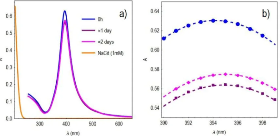
Citrate-capped silver particles (AgNPs) were synthesized by the reduction of silver perchlorate hydrate (0.1 mM, Sigma-Aldrich, 99%) in the presence of sodium borohydride (1 mM, Sigma-Aldrich, granular, 99.99% trace metals basis) and sodium citrate (0.297 mM, Sigma-Aldrich, BioUltra, ≥99.5%). Particles were left undisturbed for one hour to remove the excess of sodium borohydride, and were concentrated in a rotavap to a final concentration of 0.5 mM (~54 g/mL). The AgNPs were studied at right after up-concentration (0 h) and after nearly one day (22 h 1 day) and two days (45h  2 days) by using UV-Vis spectroscopy, transmission electron microscopy (TEM), and Taylor dispersion analysis (TDA). UV-Vis of the dispersion (Figure SI 1) was recorded with a JASCO V-670 spectrophotometer using a 10 mm path length suprasil cuvette (Hellma Analytics) at room temperature (~25 °C).

Figure SI 2. UV-Vis spectra of the AgNPs dispersed in ultrapure water. a) The optical absorbance of sodium citrate, NatCit (1mM), is

practically zero beyond 250 nm, and therefore, its presence in the dispersion does not interfere with the analysis of the taylorgrams. b) A close-up view of the peak centers, which were determined by quadratic fits (dashed lines): c(0h) = 394.16 nm, c( ≈ 1 day) = 394.87 nm, c( ≈ 2 days) = 394.97 nm.

For transmission electron microscopy (TEM), 5 L of the AgNPs dispersion was drop cast onto a 300-mesh carbon-membrane-coated copper grid, and a FEI Tecnai Spirit TEM operating at 120 kV was used to image the nanoparticles (Figure SI 3).

Figure SI 3. TEM images of the AgNPs dispersed in ultrapure water right after synthesis and after 1 day (22h). The scale bar (100 nm) is valid for both micrographs.

The UV-Vis spectra show that the AgNPs did not aggregate, and according to TEM images, the particle system was highly polydisperse. TEM images also suggest that the particle system changed in time, e.g. the edges of particles become smoother, and the particles become even more heterogeneous both in shape and in size. This was not unexpected.2-4 _{UV-Vis spectra show a subtle} red-shift in the resonance peak as a function of time, suggesting an increase in size (or better: volume), but owing to the very high polydispersity both in size and shape, the quantification of the related particle size via Mie theory of uniform spherical NPs is contradicting.5

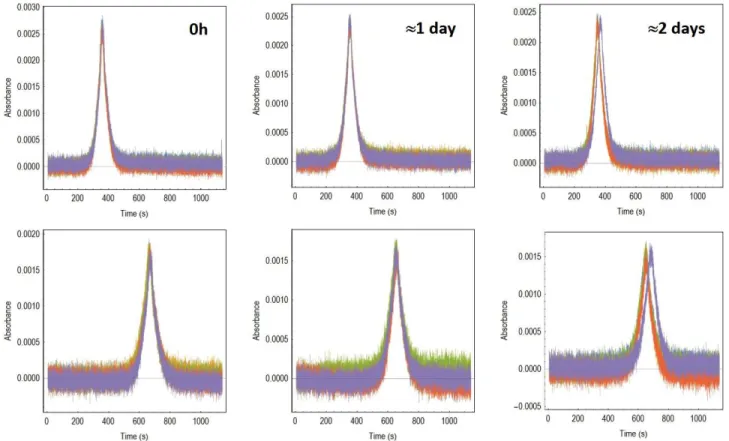
The question we are interested in answering is whether or not Taylor dispersion spectra recorded at 0h, 1 day, and 2 days are able to confirm a change in the state of the particle system, in terms of hydrodynamic radius. Therefore, taylorgrams (five independent runs of five aliquots, i.e. one run per aliquot, Figure SI 4) of the aqueous citrate-capped AgNPs dispersion were collected at a sampling rate of 20 Hz (τ = 0.05s), with an ActiPix D100 UV-Vis area imaging detector (Paraytec, York, UK), using a band-pass filter (400 nm center wavelength, 10 nm FWHM and a 32% neutral density filter (Edmund Optics, York, UK). The detector automatically corrected the intensity values for dark current, controlled the intensity of illumination (by a pulsed xenon lamp) and performed the background measurement on the respective running buffer before each run. The absorbance of the dispersion was therefore measured in the linear range of the detector throughout the measurements considering variations in illumination, background, and dark current. The aliquots with a volume of 32 nL and at room temperature (23-25 °C) were injected into a fused silica capillary (74.5±3 µm inner diameter), Polymicro Technologies, Phoenix, USA), using a capillary electrophoresis injection system (Prince 560 CE Autosampler, Prince Technologies B.V., Netherlands). The running buffer was MilliQ water. After sample injection, a pressure of (

) 90±0.9 mbar drove the samples through the capillary. The total capillary length ( ) was 145±0.05 cm, and the distances between

𝑃 𝐿

injection and the two detection points ( , ) were 37±0.05 cm and 72±0.05 cm, respectively.𝐿1 𝐿2

Figure SI 4. The taylorgrams of the AgNPs. Top and bottom panels display taylorgrams recorded at the 1st _{and 2}nd _{detection windows,}

respectively.

The trend of the baseline of an ideal taylorgram is constant and zero, however, in experimental practice the trend may deviate from zero—despite the diligent experimental care. As an attempt to minimize the influence of such deviation on the numerical analysis, the baseline was corrected—as shown in Figure SI 5—prior to analysis. After baseline correction, each taylorgram was analyzed by numerical integration to estimate the temporal mean ( ) and temporal variance ( ). The sample viscosity and sample temperature 𝑀 𝑉 were determined by combining the analyses of the two detection points, and by applying the Hagen–Poiseuille equation.1 _By determining the centers of the two taylorgrams obtained from an injection event, the capillary-cross-section-averaged mean flow velocity was determined via the ratio

(SI-1) 𝑣 = 𝐿_𝑡2― 𝐿1

2― 𝑡1

where the dispersion is recorded at two detection windows, and and are the residence times, and and are the distances 𝑡1 𝑡2 𝐿1 𝐿2 between injection and the two detection points. The fluid viscosity then can be expressed as

(SI-2) 𝜂 = 𝑌

2_𝑃

where is the driving pressure, length of capillary tube, and capillary radius. The sample temperature was determined from the 𝑃 𝐿 𝑌 viscosity, by using a function describing the temperature vs. viscosity relationship on the temperature range of 5-40 ºC: 𝑇 = 𝑐 + 𝑏/𝐿𝑛

where , , .6

(𝜂/𝑎) 𝑎 = 38.41 10―6 _{𝑃𝑎 𝑠 𝑏 = 432.91 𝐾}―1 _{𝑐 = 160.4}

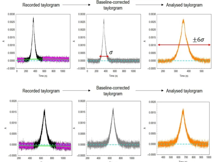
Figure SI 5. Baseline correction of taylorgrams. Baselines were estimated by fitting a cubic polynomial (solid green line) to the

peak-excluded intervals (center ± 200 s, in magenta) and were corrected by subsequent subtracting. The dashed cyan line marks the trend of a perfect baseline. The time interval used for numerical analysis was limited to a coverage factor of six, that is, ±six times the temporal width (standard deviation: ) of the baseline-corrected taylorgram.

Given that in our experiments, the duration of the pressure ramp (3s) was negligible compared to the residence times, and each aliquot volume was estimated to be less than 2% and 1% compared to the capillary volume until the first and second window, we did not apply any correction-term in the analysis, and the hydrodynamic radius determined at the 2nd _{window is} expected to be of good accuracy.7,8

The outline of our analysis is shown in Figure SI 6. Accordingly, the absorption-weighted average hydrodynamic radii (𝑟𝑝𝑜𝑙𝑦 , eq 12) of the five runs and the sampling distribution of the relative precision (Figure SI 7) is estimated via the theory →𝑟

described by eq 3 and 12-35. With a sample size equal to five, the sampling distribution of the relative error is6,9

(SI-3) 𝑓

(

)

(

(

)

)

(

(

)

)

(

)

Figure SI 6 The outline of our Taylor dispersion analysis of the AgNPs we synthesized.

Figure SI 7. The absorption-weighted average hydrodynamic radii and the related theoretical sampling distribution of the relative precisions.

The relative precisions obtained in the experiments are marked (X).

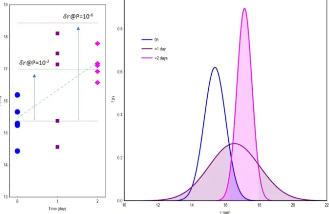
The agreement between our theoretical prediction and experimental results is good, that is, the experimental values fall within the predicted distributions. Accordingly, we accept the quality of the measurements, which are then used for estimating the resolution limits they have to offer (Figure SI 8). The absorption-weighted average hydrodynamic radii appear to follow an increasing trend with time, however, the resolution limits our measurements can offer under the conditions we had is insufficiently high to resolve the true differences in particle size, partially owing to the relatively small signal-to-noise ratio.

Are then the differences real? The estimated sampling distributions suggest that the mean values are indeed different, however, the chance of obtaining ambiguous results is not negligible because the sampling distributions overlap considerably. Apparently, either a higher number of experiments (𝑛 > 15) or higher particle concentration would have needed to resolve with high certainty the different hydrodynamic radii.

Figure SI 8. Left: The absorption-weighted average hydrodynamic radii. While the dashed line—obtained by unconstrained linear

regression—indicates an increasing trend, the resolution limits (eq 11) that these 3x5 measurements can offer is insufficient to resolve the true difference particle size, partially owing to the relatively small signal-to-noise ratio (between 20 and 30). Right: The related theoretical sampling distributions of the mean values (eq 4) indeed show considerable overlaps between the distributions, e.g. the overlap between 𝑔

@ 0h and @2days is 10.5%.

(

)

REFERENCES

(1) Lavoisier, A.; Schlaeppi, J.-M. Early Developability Screen of Therapeutic Antibody Candidates Using Taylor Dispersion Analysis and Uv Area Imaging Detection, mAbs, 2015, 7, 77-83.

(2) Kittler, S.; Greulich, C.; Diendorf, J.; Köller, M.; Epple, M. Toxicity of Silver Nanoparticles Increases During Storage Because of Slow Dissolution under Release of Silver Ions, Chemistry of Materials, 2010, 22, 4548-4554.

(3) Liu, J.; Hurt, R. H. Ion Release Kinetics and Particle Persistence in Aqueous Nano-Silver Colloids, Environmental Science & Technology, 2010, 44, 2169-2175.

(4) Zhang, W.; Yao, Y.; Sullivan, N.; Chen, Y. Modeling the Primary Size Effects of Citrate-Coated Silver Nanoparticles on Their Ion Release Kinetics, Environmental Science & Technology, 2011, 45, 4422-4428.

(5) Paramelle, D.; Sadovoy, A.; Gorelik, S.; Free, P.; Hobley, J.; Fernig, D. G. A Rapid Method to Estimate the Concentration of Citrate Capped Silver Nanoparticles from Uv-Visible Light Spectra, Analyst, 2014, 139, 4855-4861.

(6) Taladriz-Blanco, P.; Rothen-Rutishauser, B.; Petri-Fink, A.; Balog, S. Precision of Taylor Dispersion, Analytical Chemistry, 2019, 91, 9946-9951.

(7) Sharma, U.; Gleason, N. J.; Carbeck, J. D. Diffusivity of Solutes Measured in Glass Capillaries Using Taylor's Analysis of Dispersion and a Commercial Ce Instrument, Analytical Chemistry, 2005, 77, 806-813.

(8) Chamieh, J.; Oukacine, F.; Cottet, H. Taylor Dispersion Analysis with Two Detection Points on a Commercial Capillary Electrophoresis Apparatus, J Chromatogr A, 2012, 1235, 174-177.

(9) Balog, S.; Rodriguez-Lorenzo, L.; Monnier, C. A.; Michen, B.; Obiols-Rabasa, M.; Casal-Dujat, L.; Rothen-Rutishauser, B.; Petri-Fink, A.; Schurtenberger, P. Dynamic Depolarized Light Scattering of Small Round Plasmonic Nanoparticles: When Imperfection Is Only Perfect, The Journal of Physical Chemistry C, 2014, 118, 17968-17974.