HAL Id: inria-00429538
https://hal.inria.fr/inria-00429538
Submitted on 3 Nov 2009HAL is a multi-disciplinary open access
archive for the deposit and dissemination of sci-entific research documents, whether they are pub-lished or not. The documents may come from
L’archive ouverte pluridisciplinaire HAL, est destinée au dépôt et à la diffusion de documents scientifiques de niveau recherche, publiés ou non, émanant des établissements d’enseignement et de
Causal Message Sequence Charts
Thomas Gazagnaire, Blaise Genest, Loïc Hélouët, P.S. Thiagarajan, Shaofa
Yang
To cite this version:
Thomas Gazagnaire, Blaise Genest, Loïc Hélouët, P.S. Thiagarajan, Shaofa Yang. Causal Message Sequence Charts. Theoretical Computer Science, Elsevier, 2009, 38 p. �inria-00429538�
Causal Message Sequence Charts
Thomas Gazagnaire
1Citrix Systems R&D Ltd., UK
Blaise Genest
IRISA/CNRS, France
Lo¨ıc H´elou¨et
IRISA/INRIA, France
P.S. Thiagarajan
School of Computing, National University of Singapore
Shaofa Yang
1NUS, Singapore
Abstract
Scenario languages based on Message Sequence Charts (MSCs) have been wide-ly studied in the last decade [21,20,3,15,12,19,14]. The high expressive power of MSCs renders many basic problems concerning these languages undecidable. How-ever, several of these problems are decidable for languages that possess a behavioral property called “existentially bounded”. Unfortunately , collections of scenarios out-side this class are frequently exhibited by systems such as sliding window protocols. We propose here an extension of MSCs called causal Message Sequence Charts and a natural mechanism for defining languages of causal MSCs called causal HMSCs (CaHMSCs). These languages preserve decidable properties without requiring exis-tential bounds. Further, they can model collections of scenarios generated by sliding window protocols. We establish here the basic theory of CaHMSCs as well as the expressive power and complexity of decision procedures for various subclasses of CaHMSCs. We also illustrate the modeling power of our formalism with the help of a realistic example based on the TCP sliding window feature.
1 Introduction
Scenario languages based on Message Sequence Charts (MSCs) have met con-siderable interest in the last decade. The attractiveness of this notation derives from two of its major characteristics. Firstly, MSCs have a simple and appeal-ing graphical representation based on just a few concepts: processes, messages and internal actions. Secondly, from a mathematical standpoint, scenario lan-guages admit an elegant formalization: they can be defined as lanlan-guages gen-erated by finite-state automata over an alphabet of MSCs. These automata are usually called High-level Message Sequence Charts (HMSCs) [16].
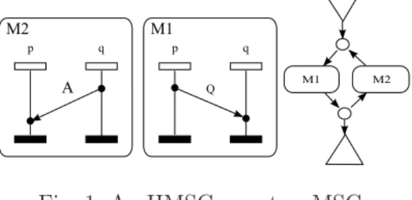
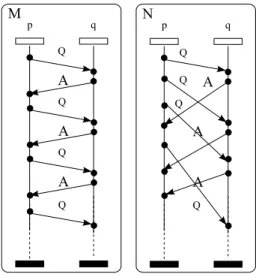
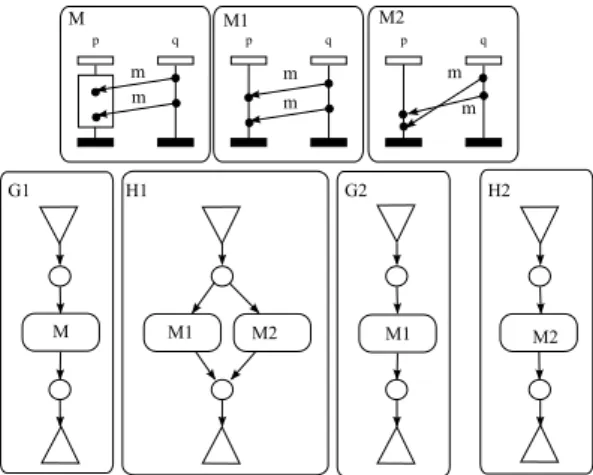
An MSC is a restricted kind of labelled partial order and an HMSC is a generator of a set of MSCs, that is, a language of MSCs. For example, the MSC M shown in Figure 2 is a member of the MSC language generated by the HMSC of Figure 1 while the MSC N shown in Figure2 is not.
Fig. 1. An HMSC over two MSCs
HMSCs are very expressive and hence a number of basic problems associated with them cannot be solved effectively. For instance, it is undecidable whether two HMSCs generate the same collection of MSCs [21] or whether an HMSC generates a regular MSC language; an MSC language is regular if the collection of all the linearizations of all the MSCs in the language is a regular string language in the usual sense. Consequently, subclasses of HMSCs have been identified [20,3,12] and studied.
On the other hand, a basic limitation of HMSCs is that their MSC languages are finitely generated. More precisely, each MSC in the language can be de-fined as the sequential composition of elements chosen from a fixed finite set of MSCs [19]. However, the behaviors of many protocols constitute MSC lan-guages that are not finitely generated. This occurs for example with scenarios generated by the alternating bit protocol. Such protocols can induce a collec-tion of braids like N in Figure 2which cannot be finitely generated.
Email addresses: [email protected] (Thomas Gazagnaire), [email protected](Blaise Genest), [email protected] (Lo¨ıc H´elou¨et), [email protected] (P.S. Thiagarajan),
[email protected](Shaofa Yang).
One way to handle this is to work with the so called safe compositional HMSCs in which message emissions and receptions are decoupled in individual MSCs but matched up at the time of composition, so as to yield an MSC. Composi-tional HMSCs are however notaComposi-tionally awkward and do not possess the visual appeal of HMSCs. Furthermore the general class of compositional HMSC lan-guages embeds the full expressive power of communicating automata [5] and consequently inherits all their undecidability results.
Fig. 2. Two MSCs M and N
This paper proposes a new approach to increase the modeling power of HMSCs in a tractable manner. We first extend the notion of an MSC to a causal MSC in which the events belonging to each lifeline (process), instead of being linearly ordered, are allowed to be partially ordered. To gain modelling power, we do not impose any serious restrictions on the nature of this partial order. However, we assume a suitable Mazurkiewicz trace alphabet [8] for each lifeline and use this to define a composition operation for causal MSCs. This leads to the notion of causal HMSCs.
A property called existential boundedness [11] leads to a powerful proof tech-nique for establishing decidability results for HMSCs. Informally, this property states that there is a uniform upper bound K such that for every MSC in the language there exists an execution along which -from start to finish- all FIFO channels remain K-bounded. On the other hand, when all executions of all MSCs in a language can occur within a fixed upper bound K on channels, the corresponding property is called universally bounded. A causal HMSC (i.e. the MSC language associated with a causal HMSC) is a priori not existentially bounded. Hence the proof method cited above can not be used to obtain the desired decidablity results. Instead, we need to generalize the methods of [20] and of [12] in a non-trivial way.
Our fist major result is to formulate natural -and decidable- structural con-ditions and to show that causal HMSCs satisfying these concon-ditions generate
MSC languages that are regular. Our second major result is that the inclusion problem for causal HMSCs (i.e. given two causal HMSCs, whether the MSC language defined by the first one is included in the MSC langauge of the other) is decidable for causal HMSCs using the same Mazurkiewicz trace alphabets, provided at least one of them has the structural property known as globally-cooperative. Furthermore, we prove that the restriction that the two causal HMSCs have identical Mazurkiewicz trace alphabets associated with them is necessary. These results constitute a non-trivial extension for causal HMSCs of comparable results on HMSCs [20,3,14] and [12]. In addition, we identify the property called “window-bounded” which appears to be an important ingredi-ent of the “braid”-like MSC languages generated by many protocols. Basically, this property bounds the number of messages a process p can send to a process q before having received an acknowledgement to the earliest message. We show it is decidable if a causal HMSC generates a window-bounded MSC language. Finally, we compare the expressive power of languages based on causal HMSCs with other known HMSC-based language and give a detailed example based on the TCP protocol to illustrate the modeling potential of causal HMSCs. This paper is an extended version of the work presented in [10] and contains several important changes and improvements. Specifically, the definition of s-regularity for causal HMSCs has been weakened. As a result, causal HMSCs which were not s-regular according to [10] -and in fact not even globally-coperative- are deemed to be s-regular under the weakened definition. We have also included here complete proofs and have added a detailed example. In the next section we introduce causal MSCs and causal HMSCs. We also de-fine the means for associating an ordinary MSC language with a causal HMSC. In the subsequent section we develop the basic theory of causal HMSCs. To this end, we identify the subclasses of s-regular (syntactically regular) and globally-cooperative causal HMSCs and develop our decidability results. In section4, we identify the “window-bounded” property, and show that one can decide if a causal HMSC generates a window-bounded MSC language. In sec-tion 5we compare the expressive power of languages based on causal HMSCs with other known HMSC-based language classes. Finally, in section6, we give a detailed example based on the TCP protocol to illustrate the modeling po-tential of causal HMSCs.
2 MSCs, causal MSCs and causal HMSCs
Through the rest of the paper, we fix a finite nonempty set P of process names with |P| > 1. For convenience, we let p, q range over P and drop the subscript p ∈ P when there is no confusion. We also fix finite nonempty sets Msg, Act of message types and internal action names respectively. We define
the alphabets Σ! = {p!q(m) | p, q ∈ P, p 6= q, m ∈ Msg}, Σ? = {p?q(m) |
p, q ∈ P, p 6= q, m ∈ Msg}, and Σact = {p(a) | p ∈ P, a ∈ Act}. The letter
p!q(m) means the sending of a message with content m from p to q; p?q(m) the reception of a message of content m at p from q; and p(a) the execution of an internal action a by process p. Let Σ = Σ!∪Σ?∪Σact. We define the location of
a letter α in Σ, denoted loc(α), by loc(p!q(m)) = p = loc(p?q(m)) = loc(p(a)). For each process p in P, we set Σp = {α ∈ Σ | loc(α) = p}.
Definition 1 A causal MSC over (P, Σ) is a structure B = (E, λ, {⊑p}, ≪),
where E is a finite nonempty set of events, λ : E → Σ is a labelling function, and the following conditions hold:
• For each process p, ⊑p ⊆ Ep× Ep is a partial order, where Ep = {e ∈ E |
λ(e) ∈ Σp}. We let ⊑bp ⊆ Ep× Ep denote the least relation such that ⊑p is
the reflexive and transitive closure of ⊑bp (⊑bp is the Hasse diagram of ⊑p). • ≪ ⊆ E!× E? is a bijection, where E!= {e ∈ E | λ(e) ∈ Σ!} and E? = {e ∈
E | λ(e) ∈ Σ?}. For each e ≪ e′, λ(e) = p!q(m) iff λ(e′) = q?p(m).
• The transitive closure ≤ of the relation ³ S
p∈P
⊑p
´
∪ ≪ is a partial order. For each p, the relation ⊑p dictates the “causal” order in which events of
Ep may be executed. The relation ≪ identifies pairs of message-emission and
message-reception events. We say that the causal MSC B is weak-FIFO iff for any e ≪ f , e′ ≪ f′ such that λ(e) = λ(e′) = p!q(m′) (and thus λ(f ) = λ(f′) =
q?p(m)), we have either e ⊑p e′ and f ⊑q f′; or e′ ⊑p e and f′ ⊑q f . In
weak-FIFO2 scenarios, messages of the same content between two given processes
cannot overtake. Note however that messages of different kind between two processes can overtake. Note that we do not demand a priori that a causal MSC must be weak FIFO. Testing (weak) fifoness of a causal MSC of size b can be done in at most O(b2
8 − b
4), by considering all pairs of messages in the
MSC.
Let B = (E, λ, {⊑p}, ≪) be a causal MSC. We shall write |B| for |E| and refer
to |B| as the size of B. A linearization of B is a word a1a2. . . aℓ over Σ such
that E = {e1, . . . , eℓ} with λ(ei) = ai for each i; and ei ≤ ej implies i ≤ j for
any i, j. We let Lin(B) denote the set of linearizations of B. Clearly, Lin(B) is nonempty. We set Alph(B) = {λ(e) | e ∈ E}, and Alphp(B) = Alph(B) ∩ Σp
for each p.
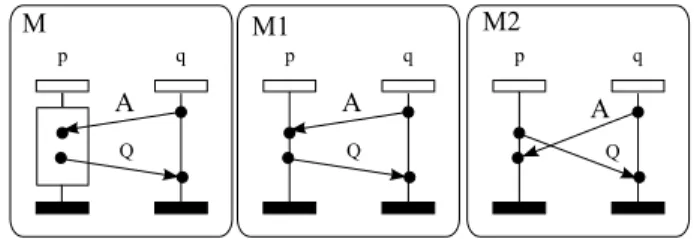
The leftmost part of Figure3depicts a causal MSC M . In this diagram, we en-close events of each process p in a vertical box and show the partial order ⊑p in
the standard way. In case ⊑pis a total order, we place events of p along a verti-2 A different notion called strong FIFO that does not allow overtakings of messages
between two given processes of different content is also frequently used in the MSC literature.
cal line with the minimum events at the top and omit the box. In particular, in M , the two events on p are not ordered (i.e.⊑bp is empty) and ⊑q is a total or-der. Members of ≪ are indicated by horizontal or downward-sloping arrows la-belled with the transmitted message. Both words p!q(Q).q!p(A).q?p(Q).p?q(A) and q!p(A).p?q(A).p!q(Q).q?p(Q) are linearizations of M .
An MSC B = (E, λ, {⊑p}, ≪) is defined in the same way as a causal MSC
except that every ⊑p is required to be a total order. In an MSC B, the
rela-tion ⊑p must be interpreted as the visually observed order of events in one
sequential execution of p. Let B′ = (E′, λ′, {⊑′
p}, ≪′) be a causal MSC. Then
we say the MSC B is a visual extension of B′ if E′ = E, λ′ = λ, ⊑′
p ⊆ ⊑p and
≪′ = ≪. We let Vis(B′) denote the set of visual extensions of B′.
Fig. 3. A causal MSC M and its visual extensions M 1, M 2.
In Figure 3, Vis(M ) consists of MSCs M 1, M 2. The initial idea of visual or-dering comes from [2], that notices that depending on the interpretation of an MSC, for example when a lifeline describes a physical entity in a network, imposing an ordering on message receptions is not possible. Hence, [2] distin-guishes two orderings on MSCs: a visual order (that is the usual order used for MSCs), that comes from the relative order of events along an instance line, and a causal order, that is weaker, and does not impose any ordering among consecutive receptions.
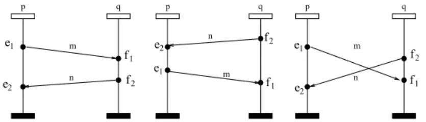
Note that the set of visual extensions of a causal MSC B is not necessarily the union of instance per instance linearizations, as an extension of a causal MSC must remain a MSC, ie. the relation among the events has to remain a partial order. Consider for example, the causal MSC B of Figure 4, and its visual extensions in Figure5: in any visual extension V = ({e1, e2, f1, f2}, λ, {⊑p, ⊑q
}, ≪) ∈ V is(B) we cannot have e2 ⊑p e1 and f1 ⊑qf2 at the same time.
We next define a concatenation operation for causal MSCs. Unlike for usual MSCs, events of a same process need not be dependent. To express whether there should be a dependency or not, for each process p in P, we fix a con-current alphabet (Mazurkiewicz trace alphabet [8]) (Σp, Ip) for each process
p ∈ P, where Ip ⊆ Σp× Σp is a symmetric and irreflexive relation called the
independence relation over the alphabet of actions Σp. We denote the
depen-dence relation (Σp × Σp) − Ip by Dp. These relations are fixed for the rest of
the paper (unless explicitly stated otherwise). Following the usual definitions of Mazurkiewicz traces, for each (Σp, Ip), the associated trace equivalence
re-Fig. 4. An example of causal MSC B: the set of visual extensions of B is not the instance per instance commutative closure of any visual extension of B.
Fig. 5. Visual extensions of the causal MSC B of Figure4.
lation ∼p over Σ⋆p is the least equivalence relation such that, for any u, v in Σ⋆p
and α, β in Σp, α Ip β implies uαβv ∼p uβαv. Equivalence classes of ∼p are
called traces. For u in Σ⋆
p, we let [u]p denote the trace containing u.
Let B = (E, λ, {⊑p}, ≪) be a causal MSC. We say ⊑p respects the trace
alphabet (Σp, Ip) iff for any e, e′ ∈ Ep, the following hold:
(i) λ(e) Dp λ(e′) implies e ⊑p e′ or e′ ⊑p e
(ii) e ⊑bp e′ implies λ(e) D p λ(e′)
A causal MSC B is said to respect the trace alphabets {(Σp, Ip)}p∈P iff ⊑p
respects (Σp, Ip) for every p. In order to gain modelling power, we have allowed
each ⊑p to be any partial order, not necessarily respecting (Σp, Ip).
We shall now define the concatenation operation of causal MSCs using the trace alphabets {(Σp, Ip)}p∈P.
Definition 2 Let B = (E, λ, {⊑p}, ≪) and B′ = (E′, λ′, {⊑′p}, ≪′) be causal
MSCs. We define the concatenation of B with B′, denoted by B ⊚ B′, as the
causal MSC B′′ = (E′′, λ′′, {⊑′′
p}, ≪′′) where:
• E′′ is the disjoint union of E and E′. λ′′ is given by: λ′′(e) = λ(e) if e ∈ E,
λ′′(e) = λ′(e) if e ∈ E and ≪′′ = ≪ ∪ ≪′.
• For each p, ⊑′′
p is the transitive closure of
⊑p
[
Clearly, ⊚ is a well-defined and associative operation. Note that in case B and B′ are MSCs and D
p = Σp× Σp for every p, then the result of B ⊚ B′ is
the asynchronous concatenation (also called weak sequential composition) of B with B′ [22], which we denote by B ◦ B′. Note that when B
1 and B2 are
weak FIFO causal MSCs, then their concatenation is also weak FIFO. This property comes from the irreflexive nature of the independence relations. This remark also holds for the concatenation of MSCs. We also remark that the concatenation of causal MSCs is different from the concatenation of traces. The concatenation of trace [u]p with [v]p is the trace [uv]p. However, a causal
MSC B needs not respect {(Σp, Ip)}p∈P. Consequently, for a process p, the
projection of Lin(B) on Alphp(B) is not necessarily a trace.
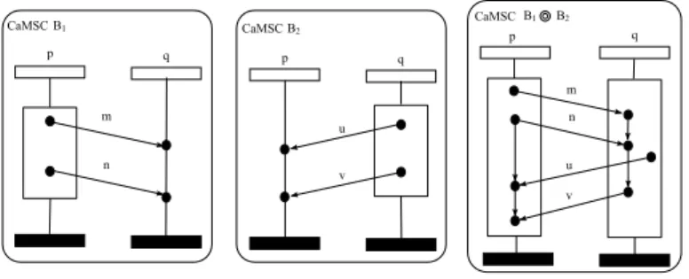
Figure6 shows an example of sequential composition of two causal MSCs B1
and B2, with the dependency relations Dp and Dq being the commutative and
reflexive closure ofn³p!q(m), p!q(n)´,³p!q(n), p?q(u)´oandn³q?p(n), q!p(v)´o respectively. Note that although the dependence relation Dp contains the pair
³
p!q(m), p!q(n)´, sendings of messages m and n by process p in B1 can be
unordered, and remain unordered after composition.
Fig. 6. Concatenation example.
An usual way to extend the composition mechanism is to use an automaton labelled by basic scenarios, to produce scenario languages. These automata are called High-level Message Sequence Charts (or HMSCs for short)[25,23] when MSCs are concatenated, and a similar construct exists for compositional Message Sequence Charts [13,11,7]. We can now define causal HMSCs. Recall that we have fixed a set P of process names and a family {(Σp, Ip)}p∈P of
Mazurkiewicz trace alphabets.
Definition 3 A causal HMSC over (P, {(Σp, Ip)}p∈P) is a structure H =
(N, Nin, B, −→, Nfi) where N is a finite nonempty set of nodes, Nin ⊆ N the
set of initial nodes, B a finite nonempty set of causal MSCs, −→ ⊆ N × B × N the transition relation, and Nfi ⊆ N the set of final nodes.
A path in the causal HMSC H is a sequence ρ = n0 B1
−→ n1 B2
−→ · · · Bℓ
−→ nℓ .
If n0 = nℓ, then we say ρ is a cycle. The path ρ is accepting iff n0 ∈ Nin and
nℓ ∈ Nfi. The causal MSC generated by ρ, denoted ⊚(ρ), is B1⊚B2⊚· · · ⊚ Bℓ.
of H. We also set Vis(H) = S{Vis(M ) | M ∈ cMSC (H)} and Lin(H) = S
{Lin(M ) | M ∈ cMSC (H)}. Obviously, Lin(H) is also equal toS{Lin(M ) | M ∈ Vis(H)}. We shall refer to cMSC (H), Vis(H), Lin(H), respectively, as the causal language, visual language and linearization language of H.
An HMSC H = (N, Nin, B, −→, Nfi) is defined in the same way as a causal
HMSC except that B is a finite set of MSCs, and that the concatenation op-eration used to produce MSC languages is the weak sequential composition ◦. HMSCs can then be considered as causal HMSCs labelled with MSCs, and equipped with empty independence relation (for every p ∈ P, Ip = ∅). Hence,
a path ρ of H generates an MSC by concatenating the MSCs along ρ with operation ◦. We let Vis(H) denote the set of MSCs generated by accepting paths of H with ◦, and call Vis(H) the visual language of H. Recall that an MSC language (i.e. a collection of MSCs) L is finitely generated [19] iff there exists a finite set X of MSCs satisfying the condition: for each MSC B in L, there exist B1, . . . , Bℓ in X such that B = B1◦ · · · ◦ Bℓ. Many
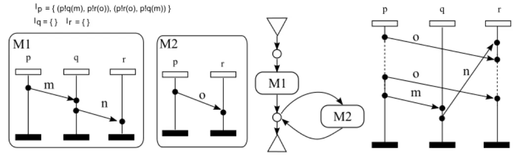
proto-cols exhibit scenario collections that are not finitely generated. For example, sliding window protocols can generate arbitrarily large MSCs repeating the communication behavior shown in MSC N of Figure 2. One basic limitation of HMSCs is that their visual languages are finitely generated. In contrast, the visual language of a causal HMSC is not necessarily finitely generat-ed. Consider for instance the HMSC H in Figure 1, and the independence relations given by: Ip = {((p!q(Q), p?q(A)), (p?q(A), p!q(Q)))} and Iq = ∅.
M 1 and M 2 can be seen as causal MSCs, and H as a causal HMSC over (P = {p, q}, {(Σp, Ip)(Σq, Iq)}). Clearly, Vis(H) is not finitely generated, as
it contains infinitely many MSCs similar to N of Figure 2. Throughout the paper, we will use the following standardized graphical convention to depict (causal) HMSCs: nodes are represented by circles, initial nodes are nodes con-nected to a downward pointing triangle, final nodes are nodes concon-nected to an upward pointing triangle, and a transition t = (n, B, n′) is represented by
an arrow decorated by a rectangle containing the (causal) MSC B.
3 Regularity and Language Inclusion for causal HMSCs
3.1 Semantics for causal HMSCs
As things stand, a causal HMSC H defines three syntactically different lan-guages, namely its linearization language Lin(H), its visual (MSC) language Vis(H) and its causal MSC language cMSC (H). The next proposition shows that they are also semantically different in general. It also identifies the re-strictions under which they match semantically.
Proposition 1 Let H, H′ be two causal HMSCs over the same family of trace
alphabets {(Σp, Ip)}p∈P. Consider the following six hypotheses:
(i) cMSC (H) = cMSC (H′) (i)’ cMSC (H) ∩ cMSC (H′) 6= ∅
(ii) Vis(H) = Vis(H′) (ii)’ Vis(H) ∩ Vis(H′) 6= ∅
(iii) Lin(H) = Lin(H′) (iii)’ Lin(H) ∩ Lin(H′) 6= ∅
Then we have:
• (i) ⇒ (ii), (i)′ ⇒ (ii)′, (ii) ⇒ (iii) and (ii)′ ⇒ (iii)′ but the converses
do not hold in general.
• If every causal MSC labelling transitions of H and H′ respects {(Σ
p, Ip)}p∈P,
then (i) ⇔ (ii) and (i)′ ⇔ (ii)′.
• If every causal MSC labelling transitions of H and H′ is weak FIFO, then
(ii) ⇔ (iii) and (ii)′ ⇔ (iii)′.
Proof:
• The implications (i) =⇒ (ii) and (ii) =⇒ (iii) follow from the defini-tions. However, as shown in Figure 7, Vis(G1) = Vis(H1) but cMSC (G1) 6=
cMSC (H1). And Lin(G2) = Lin(H2) but Vis(G2) 6= Vis(H2). Note that
the independence relations are immaterial in these examples. • If every causal MSC labelling transitions of H and H′ respects {(Σ
p, Ip)}p∈P,
then one can define an equivalence relation M ≡ M′ on MSCs iff there
exists a causal MSC C with M, M′ ∈ Vis(C). Then, for any causal MSC B
in cMSC (H)ScMSC (H′), Vis(B) is an equivalence class of that relation,
and (i) ⇔ (ii) and (i)′ ⇔ (ii)′.
• If every causal MSC labelling transitions of H and H′ is weak FIFO, as
remarked earlier, we know that all MSCs in V is(H)∪V is(H′) are weak FIFO
since the independence relations are irreflexive. Now, for each linearization w, one can reconstruct a unique weak FIFO MSC. Hence, if Lin(M1) =
Lin(M2) for M1 and M2 are in V is(H) ∪ Vis(H′), they are weak FIFO, and
we necessarily have M1 = M2, and (ii) ⇔ (iii) and (ii)′ ⇔ (iii)′.
¤
For most purposes, the relevant semantics for a causal HMSC seems to be its visual language. However in the following we focus first in section 3.2 on the linearization language properties of causal HMSCs. Then, we focus in section 3.3 on the causal language properties. Using the above proposition 1, it is then straightforward to translate these properties to the visual language of causal HMSCs, when the right hypothesis apply.
Fig. 7. Relations between linearizations, visual extensions and causal orders 3.2 Regular sets of linearizations
It is undecidable in general whether an HMSC has a regular linearization language [20]. In the literature, a subclass of HMSCs called regular [20] (or bounded [3]) HMSCs, has been identified. In this paper, to avoid overloading “regular”, we shall refer to this syntactic property as “s-regular”. The im-portance of this property lies in the fact that linearization language of every s-regular HMSC is regular. Furthermore, one can effectively decide whether an HMSC is s-regular. Our goal is to extend these results to causal HMSCs. The key notion of characterizing s-regular HMSCs is that of the communi-cation graph of an MSC. The communicommuni-cation graph captures intuitively the structure of information exchanges among processes in an MSC. Given an MSC M , its communication graph is a directed graph that has processes of M as vertices, and contains an edge from p to q if p sends a message to q somewhere in M . Given an HMSC H, we shall say that M is a cycle-MSC of H if there is a cycle in H such that M is obtained by concatenating the MSCs encountered along this cycle. H is said to be s-regular iff the communication graph of every cycle-MSC of H is strongly connected. H is said to be globally-cooperative [19] in case the communication graph of every cycle MSC of H is connected.
We can define a similar notion for causal MSCs. As processes do not neces-sarily impose an ordering on events, it is natural to focus on the associated Mazurkiewicz alphabet. Thus the communication graph is defined w.r.t the dependency relations {Dp}p∈P used for the concatenation while the
dependen-cies among letters of the same process are disregarded.
Definition 4 Let B = (E, λ, {⊑p}, ≪) be a causal MSC. The communication
graph of B is denoted by CGB, and is the directed graph (Q, Ã), where Q =
• x = p!q(m) and y = q?p(m) for some p, q ∈ P and m ∈ Msg, or • xDpy.
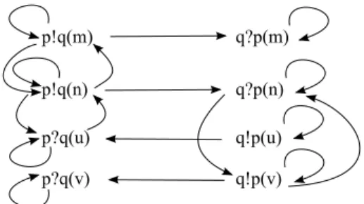
Fig. 8. Communication graph for causal MSC B1⊚B2 of Figure6.
The example of figure 8 shows the communication graph for the causal MSC B1 ⊚ B2 in Figure 6. For instance, there are arrows between q?p(n) and
q!p(v) since q?p(n) Dq q!p(v). However, there is no arrow between q?p(m) and
q?p(n), even though some events of B1 ⊚B2 labeled by q?p(m) and q?p(n)
are dependent. Note that for a pair of causal MSCs B, B′, the communication
graph CGB⊚B′ = (Q, Ã) can be computed from the communication graphs
CGB = (QB, ÃB) and CGB′ = (QB′, ÃB′) as follows: Q = QB ∪ QB′ and
Ã= ÃB∪ ÃB′ ∪
³
Q2 ∩ S p∈PDp
´
. Hence, for a fixed set of independence rela-tions, if a causal MSC B is obtained by sequential composition, that is B = B1⊚B2⊚· · ·⊚Bk, then the communication graph of B does not depend on the
respective ordering of B1, · · · Bk, nor on the number of occurrences of each Bi.
Hence, for any permutation f on 1..k and any B′ = B
f(1)⊚Bf(2)⊚· · · ⊚ Bf(k),
we have that CGB = CGB′.
In the sequel, we will say that the causal MSC B is tight iff its communication graph CGB is weakly connected. We say that B is rigid iff its communication
graph is strongly connected. We will focus here on rigidity and study the notion of tightness in section3.3.
Definition 5 Let H = (N, Nin, B, Nfi, −→) be a causal HMSC. We say that
H is s-regular (resp. globally-cooperative) iff for every cycle ρ in H, the causal MSC ⊚(ρ) is rigid (resp. tight).
It is easy to see that the simple protocol modeled by the causal HMSC of Fig-ure 9is regular, since the only elementary cycle is labeled by two local events a, b, one message from p to q and one message from q to p. The communication graph associated to this elementary cycle is strongly connected. Note that the visual language of this causal HMSC is not finitely generated, as messages m and n can cross between two occurrences of a and b.
There can be infinitely many cycles in H, hence Definition 5 does not give automatically an algorithm to check whether a causal HMSC is s-regular or globally-cooperative. However, we can use the following equivalent definition
Fig. 9. A non finitely generated s-regular causal HMSC and its communication graph.
to obtain an algorithm: H is s-regular (resp. globally-cooperative) iff for every strongly connected subgraph G of H with {B1, . . . , Bℓ} being the set of causal
MSCs appearing in G, we have B1⊚. . . ⊚ Bℓ is rigid (resp. tight). As already
discussed, the rigidity of B1⊚. . . ⊚ Bℓ does not depend on the order in which
B1, . . . , Bℓare listed. This leads to a co-NP-complete algorithm to test whether
a causal HMSC is s-regular.
Theorem 1 Let H = (N, Nin, B, −→, Nfi) be a causal HMSC. Testing whether
H is s-regular (respectively globally-cooperative) can be done in time O((|N |2+
|Σ|2) · 2|B|). Furthermore these problems are co-NP complete.
Proof: We use the ideas in the proofs of [20,12], improving the deterministic complexity implied by the proof in [12], which was exponential in the number of transitions of the HMSC (there is at least one transition per label (else we can delete the useless labels)).
We first guess a subset X = {B1, · · · Bk} ⊆ B of causal MSCs and check
that the communication graph of B1 ⊚· · · ⊚ Bk is not strongly connected
(respectively disconnected). Using Tarjan’s algorithm [26], this can be done in time linear in the number of edges of the communicating graph, that is quadratic in |Σ|. Then, we decompose the graph HX into maximal strongly
connected components in time O(|N |2) using Tarjan again, where H
X is the
restriction of H to transitions labeled by causal MSCs in X. Then it suffices to check in time |N |2whether one of this maximal strongly connected component
uses all the labels from X. If it is the case, then we have a witness that H is not s-regular (resp. globally-cooperative). We thus obtain a co-NP algorithm. As there are 2|B| subsets X, this gives the deterministic time complexity.
The hardness part follows directly from the co-NP hardness result in [20]. As already mentioned, any HMSC can be seen as a causal HMSC where the independence relation of each process is empty. That is, checking whether such causal HMSC are globally-cooperative or s-regular is equivalent to checking global cooperativeness or regularity of the HMSC. These problems being
co-NP complete, we get the co-co-NP hardness. ¤
Theorem 2 Let H = (N, Nin, B, Nfi, −→) be a s-regular causal HMSC. Then
Lin(H) is a regular subset of Σ⋆, i.e. we can build an automaton A
H over Σ
that recognizes Lin(H). Furthermore, the number of states of AH is at most
in ³
|N |2 · 2|Σ|· (Σ + 1)K·M · 2f(K·M )´K ,
where K = |N | · |Σ| · 2|B|, M = max{|B| | B ∈ B} (recall that |B| denotes the
size of the causal MSC B)nd the function f is given by f (n) = 14n2 + 3 2n +
O(log2n).
In [18], the regularity of linearization languages of s-regular HMSC was proved by using an encoding into connected traces and building a finite state automa-ton which recognizes such connected traces. In our case, finding such embed-ding into Mazurkiewicz traces seems impossible due to the fact that causal MSCs need not be FIFO. Instead, we shall use techniques from the proof of regularity of trace closures of loop-connected automata from [8,20].
The rest of this subsection is devoted to the proof of Theorem 2. We fix a s-regular causal HMSC H as in the theorem, and show the construction of the finite state automaton AH over Σ which accepts Lin(H).
First, we establish some technical results.
Lemma 1 Let ρ = θ1. . . θ2. . . θ|Σ| be a path of H, where for each i = 1 . . . |Σ|,
the subpath θi = ni,0 Bi,1
−→ ni,1. . . ni,ℓi−1
Bi,ℓi
−→ ni,0 is a cycle (these cycles need
not be contiguous). Suppose further that the sets Bbi = {Bi,1, . . . , Bi,ℓi}, i =
1, . . . , |Σ|, are equal. Let e be an event in ⊚(θ1) and e′ an event in ⊚(θ|Σ|). Let
⊚(ρ) = (E, λ, {⊑p}, ≪). Then we have e ≤ e′.
Proof:
First of all notice that when (σ, σ′) is an edge of CG
B, then for every causal
MSC B′, in the causal MSC B ⊚ B′, every event e of B such that λ(e) = σ
precedes all events e′ of B′ such that λ(e′) = σ′. Indeed, if σ and σ′ belong
to the same Σp, then (σ, σ′) is an edge of CGB if and only if σDpσ′, and we
necessarily have e ≤ e′ in B ⊚ B′. Similarly, if σ and σ′ label events located
on different processes, then σ is of the form p!q(m) and σ′ of the form q?p(m).
Hence, there exists an event e′′ of B such that e ≪ e′′ and λ(e′′) = σ′. As
the dependence relations are reflexive, we also have e′′≤ e′. Similarly, for two
cycles θi,θi+1 of ρ, if (σ, σ′) is an edge of CGBi,1⊚···⊚Bi,li, then all events in
⊚(θi) labelled by σ precede events of ⊚(θi+1) labelled by σ′. As H is rigid, CGBi,1⊚···Bi,li is strongly connected, and contains a path (σ1, σ2) · · · (σk−1, σk)
i ∈ 1..|Σ| for each cycle such that λ(ei) = σi and e = e1 ≤ e2 ≤ · · · ≤ e|Σ| = e′. ¤ Let ρ = n0 B1 −→ · · · Bℓ −→ nℓ be a path in H, where Bi = (Ei, λi, {⊑ip}, ≪i)
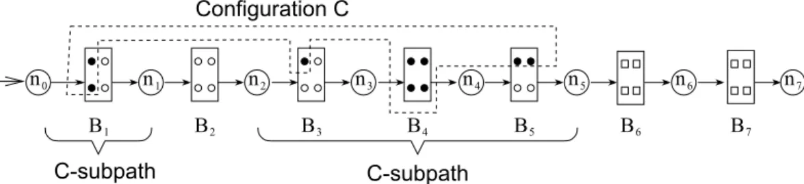
for i = 1, . . . , ℓ. Let ⊚(ρ) = (E, λ, {⊑p}, ≪, ≤). A configuration of ρ is a
≤-closed subset of E. Let C be a configuration of ρ. A C-subpath of ρ is a maximal subpath ̺ = nu
Bu+1
−→ . . . Bu′
−→ nu′, such that C ∩ Ei 6= ∅ for
each i = u, . . . , u′. For such a C-subpath ̺, we define its C-residue to be
the set (Eu+1 ∪ Eu+2 ∪ · · · ∪ Eu′) − C. Figure 10 illustrates these notions
for a path ρ = n0 B1 −→ n1 B2 −→ n2 B3 −→ n3 B4 −→ n4 B5 −→ n5 B6 −→ n6 B7 −→ n7.
Each causal MSC is represented by a rectangle. Events in the configuration C are indicated by small filled circles, events not in C but the C-residues are indicated by small blank circles, and events that are not in C nor in its residues are indicated by blank squares. Note that the configuration contains only events from B1, B3, B4 and B5. The two C-subpaths identified on Figure10are
the sequences of transitions ρ1 = n0 B1 −→ n1 and ρ2 = n2 B3 −→ n3 B4 −→ n4 B5 −→ n5
that provide the events appearing in C. One can also notice from this example that C-subpaths do not depend on the length of a the considered path, and that the suffix of each path that does not contain an event in C can be ignored.
Fig. 10. An example of path, a configuration C, and its C-subpaths. Lemma 2 Let ρ be a path in H and C be a configuration of ρ. Then, (i) The number of C-subpaths of ρ is at most Ksubpath = |N | · |Σ| · 2|B|.
(ii) Let ̺ be a C-subpath of ρ. Then the number of events in the C-residue of ̺ is at most Kresidue = |N | · |Σ| · 2|B|· max{|B| | B ∈ B}.
Proof:
(i) Suppose the contrary. Let K = |Σ| · 2|B|. We can find K + 1 C-subpaths
whose ending nodes are equal. Let the indices of these K +1 ending nodes be i1 < i2 < . . . < iK+1. For h = 1, . . . , K, let θh be the subpath of ρ from nih
to nih+1; and letBbh be the set of causal MSCs appearing in θh. Hence we can
find θj1, θj2, . . ., θj|Σ|, j1 < j2 < . . . < j|Σ|, such that Bbj1 =Bbj2 = . . . =Bbj|Σ|.
Pick an event e from ⊚(θj1) with e /∈ C. Such an e exists, since, for example,
none of the events in the first causal MSC appearing in θj1 is in C. Pick an
event e′ from ⊚(θ
j|Σ|) with e
This leads to a contradiction, since C is ≤-closed. (ii) Let ̺ = ni
Bi+1
−→ . . . Bi′
−→ ni′. LetEbj = Ej− C for j = i + 1, . . . , i′. By similar
arguments as in (i), it is easy to show that among Ebi+1, . . ., Ebi′, at most
|N | · |Σ| · 2|B| of them are nonempty. The claim then follows.
¤
We are now ready to define the finite state automaton AH = (S, Sin, Σ, Sfi, ⇒)
which accepts Lin(H). As usual, S will be the set of states, Sin ⊆ S the
initial states, =⇒ ⊆ S × Σ × S the transition relation, and Sfi ⊆ S the
final states. Fix Ksubpath, Kresidue to be the constants defined in Lemma 2. If
B = (E, λ, {⊑p}, ≪) is a causal MSC and E′ a subset of E, then we define the
restriction of B to E′ to be the causal MSC B′ = (E′, λ′, {⊑′
p}, ≪′) as follows.
As expected, λ′ is the restriction of λ to E′; for each p, ⊑′
p is the restriction
of ⊑p to (E′∩ Ep) × (E′∩ Ep); and ≪′ is the restriction of ≪ to E′.
Intuitively, for a word σ in Σ⋆, A
H guesses an accepting path ρ of H and checks
whether σ is in Lin(⊚(ρ)). After reading a prefix σ′ of σ, A
H memorizes a
sequence of subpaths from which σ′ was “linearized” (i.e the C-subpath of
a path ρ such that C is a configuration reached after reading σ′ and ⊚(ρ)
contains C). With Lemma 2, it will become clear later that at any time, we should remember at most Ksubpath such subpaths. Moreover, for each subpath,
we need to know only a bounded amount of information, which will be stored in a data structure called “segment”.
A causal MSC B = (E, λ, {⊑p}, ≪) is of size lower than K if |E| ≤ K. A
segment is a tuple (n, Γ, W, n′), where n, n′ ∈ N , Γ is a nonempty subset of Σ,
and W is either a non-empty causal MSC of size lower than Kresidue, or the
special symbol ⊥. The state set S of AH is the collection of finite sequences
θ1θ2. . . θℓ, 0 ≤ ℓ ≤ Ksubpath, where each θi is a segment. Intuitively, a segment
(n, Γ, W, n′) keeps track of a subpath ̺ of H which starts at n and ends at
n′. Γ is the collection of letters of events in ⊚(̺) that have been “linearized”. Finally, W is the restriction of ⊚(̺) to the set of events in ⊚(̺) that are not yet linearized. In case all events in ⊚(̺) have been linearized, we set W = ⊥. For convenience, we extend the operator ⊚ by: W ⊚ ⊥ = ⊥ ⊚ W = W for any causal MSC W ; and ⊥ ⊚ ⊥ = ⊥.
We define AH = (S, Sin, Σ, Sfi, =⇒) as follows:
• As mentioned above, S is the collection of finite sequence of at most Ksubpath
segments.
• The initial state set is Sin = {ε}, where ε is the null sequence.
• A state is final iff it consists of a single segment θ = (n, Γ, ⊥, n′) such that
n ∈ Nin and n′ ∈ Nfi (and Γ is any nonempty subset of Σ).
conditions.
—Condition (i):
Suppose n −→ nB ′ where B = (E, λ, {⊑
p}, ≪, ≤). Let e be a minimal
event in B (with respect to ≤) and let a = λ(e). Let θ = (n, Γ, W, n′) where
Γ = {a}. Let R = E − {e}. If R is nonempty, then W is the restriction of B to R; otherwise we set W = ⊥. Suppose s = θ1. . . θkθk+1. . . θℓ is a state in
S where θi = (ni, Γi, Wi, n′i) for each i. Suppose further that, e is a minimal
event in W1⊚W2 ⊚. . . ⊚ Wk⊚W .
· (“create a new segment”) Let ˆs = θ1. . . θkθθk+1. . . θℓ. If ˆs is in S, then
s=⇒ ˆa s. In particular, for the initial state ε, we have ε=⇒ θ.a · (“add to the beginning of a segment”) Suppose n′ = n
k+1. Let ˆθ = (n, Γ ∪
Γk+1,W , nc ′k+1), where W = W ⊚ Wc k+1. Let ˆs = θ1. . . θkθθˆ k+2. . . θℓ. If ˆs is
in S, then s =⇒ ˆa s.
· (“append to the end of a segment”) Suppose n = n′
k. Let ˆθ = (nk, Γk ∪
Γ,W , nc ′), whereW = Wc
k⊚W . Let ˆs = θ1. . . θk−1θθˆ k+1. . . θℓ. If ˆs is in S,
then s=⇒ ˆa s.
· (“glue two segments”) Suppose n = n′
kand n′ = nk+1. Let ˆθ = (nk, Γk∪Γ∪
Γk+1,W , nc ′k+1), whereW = Wc k⊚W ⊚Wk+1. Let ˆs be θ1. . . θk−1θθˆ k+2. . . θℓ.
If ˆs is in S, then s=⇒ ˆa s. —Condition (ii):
Suppose s = θ1. . . θkθk+1. . . θℓ is a state in S where θi = (ni, Γi, Wi, n′i)
for i = 1, 2, . . . , ℓ. Suppose Wk 6= ⊥. Let Wk = (Rk, ηk, {⊑kp}, ≪k, ≤k) and
e a minimal event in Wk. Suppose further that e is a minimal event in
W1⊚W2⊚. . . ⊚ Wk.
Let ˆθ = (nk, Γk ∪ {a},W , nc ′k), where W is defined as follows. Letc R =b
Rk− {e}. IfR is nonempty, thenb W is the restriction of W toc R; otherwise,b
set W = ⊥. Let ˆc s = θ1. . . θk−1θθˆ k+1. . . θℓ. Then we have s a
=⇒ ˆs, where a = ηk(e). (Note that ˆs is guaranteed to be in S.)
We have now completed the construction of AH. It remains to show that AH
recognizes Lin(H).
Lemma 3 Let σ ∈ Σ⋆. Then σ is accepted by A
H iff σ is in Lin(H).
Proof: Let σ = a1a2. . . ak. Suppose σ is in Lin(H). Let ρ = n0 B1
−→ . . . Bℓ
−→ nℓ
be an accepting path in H such that σ is a linearization of ⊚(ρ). Hence we may suppose that ⊚(ρ) = (E, λ, {⊑p}, ≪, ≤) where E = {e1, e2, . . . , ek} and
λ(ei) = ai for i = 1, . . . , k. And ei ≤ ej implies i ≤ j for any i, j in {1, . . . , k}.
Consider the configurations Ci = {e1, e2, . . . , ei} for i = 1, . . . , k. For each
Ci, we can associate a state si in AH as follows. Consider a fixed Ci. Let
ρ = . . . ̺1. . . ̺2. . . ̺h. . . where ̺1, ̺2, . . ., ̺h are the Ci-subpaths of ρ. Then
we set si = θ1. . . θh where θj = (nj, Γj, Wj, n′j) with nj being the starting node
and Ci. Let Rj be the Ci-residue of ̺j. If Rj is nonempty, Wj is the causal
MSC (Rj, ηj, {⊑jp}, ≪j, ≤j) where ηj is the restriction of λ to Rj; ⊑jp is the
restriction of ⊑p to those events in Rj that belong to process p, for each p;
and ≪j the restriction of ≪ to Rj. If Rj is empty, then set Wj = ⊥. Finally,
n′
j is the ending node of ̺j.
Now it is routine (though tedious) to verify that ε a1
=⇒ s1. . . sk−1 ak
=⇒ sk is an
accepting run of AH. Conversely, given an accepting run of AH over σ, it is
straightforward to build a corresponding accepting path of H.
¤
With Lemma 3, we establish Theorem 2. As for complexity, the number of states in AH is at most (Nseg)Ksubpath, where Nseg is the maximal number of
segments. Now, Nseg is |N |2 · 2|Σ| · Nres, where Nres is the possible number
of residues. Recall that a residue is of size at most Kresidue. According to
Kleitman & Rotschild [17], the number of partial orders of size k is in 2f(k)
where f (k) = 1 4k
2+3
2k + O(log2(k)). It follows that the number of |Σ|-labeled
posets of size k is in 2f(k)· |Σ|k. All residues of size up to k can be encoded
as a labeled poset of size k with useless events, labelled by a specific label ♯. Hence the number of residues Nres is lower than 2f(Kresidue)· (|Σ| + 1)Kresidue.
Combining the above calculations then establishes the bound in theorem2on the number of states of AH.
3.3 Inclusion and Intersection of causal HMSC Languages
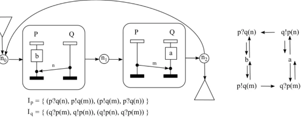
It is known that problems of inclusion, equality and non-emptiness of the inter-section of the MSC languages associated with HMSCs are all undecidable [20]. Clearly, these undecidability results also apply to the causal languages of causal HMSCs. As in the case of HMSCs, theses problems are decidable for s-regular causal HMSCs since their linearization languages are regular. It is natural to ask whether we can still obtain positive results for these prob-lems beyond the subclass of s-regular causal HMSCs. In the setting of HMSCs, one can show that for all K ≥ 0, the set of K-bounded linearizations of any globally-cooperative HMSC is regular. Moreover, for a suitable choice of K, the set of K-bounded linearizations is sufficient for effective verification [11]. Unfortunately, this result uses Kuske’s encoding [18] into traces that is based on the existence of an (existential) bound on communication channels. Conse-quently, this technique does not apply to globally-cooperative causal HMSCs, as the visual language of a causal HMSC needs not be existentially bound-ed. For instance, consider the causal HMSC H of Figure 11. It is globally-cooperative and its visual language contains MSCs shown in the right part of
Figure11: in order to receive the first message from p to r, the message from p to q and the message from q to r have to be sent and received. Hence every message from p to r has to be sent before receiving the first message from p to r, which means that H is not existentially bounded.
Fig. 11. A globally-cooperative causal HMSC that is not existentially bounded We shall instead adapt the notion of atoms [1,15] and the techniques from [12]. Definition 6 A causal MSC B is a basic part (w.r.t. the trace alphabets {(Σp, Ip)}p∈P) if there do not exist causal MSCs B1, B2 such that B = B1⊚B2.
Note that we require that the set of events of a causal MSC is not empty. Now for a causal MSC B, we define a decomposition of B to be a sequence B1· · · Bℓof basic parts such that B = B1⊚· · · ⊚ Bℓ. For a set B of basic parts,
we associate a trace alphabet (B, IB) (w.r.t. the trace alphabets {(Σp, Ip)}p∈P)
where IB is given by: B IB B′ iff for every p, for every α ∈ Alphp(B), for every
α′ ∈ Alph
p(B′), it is the case that α Ipα′. We let ∼Bbe the corresponding trace
equivalence relation and denote the trace containing a sequence u = B1. . . . .Bℓ
in B⋆ by [u]
B (or simply [u]). For a language L ⊆ B⋆, we define its trace closure
[L]B = S
u∈L[u]B. We begin by proving that the decomposition of any causal MSC
B is unique up to commutation. More precisely,
Proposition 2 Let B1. . . Bk be a decomposition of a causal MSC B. Then
the set of decompositions of B is [B1. . . Bk].
Proof: It is clear that every word in [B1. . . Bk] is a decomposition of B.
For the converse, let us suppose that there exists a decomposition B = W1⊚
W2⊚· · · ⊚ Wq such that W1. . . Wq∈ [B/ 1. . . Bk]. It means that there exists a
permutation φ and an index i with Wj = Bφ(j) for all j < i, Bφ(1)· · · Bφ(k) ∈
[B1. . . Bk], and W′ = Wi ∩ Bφ(i) 6= ∅ and W′′ = Wi \ Bφ(i) 6= ∅. It suffices
now to prove that W′ and W′′ are causal MSCs and that W
i = W′ ⊚W′′ to
get a contradiction with the fact that Wi is a basic part. By definition, the
restriction of ≪Wi to W
′ is still a bijection (a send in W′ matches a receive in
W′). It implies that the restriction of ≪
Wi to W
′′ is a bijection too. Both W′
and W′′ are thus causal MSCs. The fact that W
i = W′⊚W′′ comes from the
definition of ⊚ and from the fact that W′ ⊆ B
¤
It is thus easy to compute the (finite) set of basic parts of a causal MSC B, denoted Basic(B), since it suffices to find one of its decomposition.
Proposition 3 For a given causal MSC B, we can effectively decompose B in time O(|B|2).
Proof: Let B = (E, λ, {⊑p}, ≪). We describe the decomposition of B, which
is analogous to the technique in [15]. We consider the directed graph (E, ≤ ∪R), where R is the symmetric closure of ≪ ∪³Sp∈PR′p∪ R′′p
´ , with
Rp′ = {(e, e′) ∈ Ep × Ep | e⊑bpe′ and λ(e) Ip λ(e′)} ,
R′′p = {(e, e′) ∈ Ep× Ep | e 6⊑p e′ and e′ 6⊑p e and λ(e) Dp λ(e′)} .
Intuitively, R′
p denote pairs of events that are ordered in B, but which labels
are independent in Ip. As this ordering can not be obtained via composition,
this ordering should appear in the decomposition of B, that is e and e′ should
belong to the same basic part. Similarly, relation R′′
p contains pairs of events
that are unordered in B, but which labels are dependent.
For each strongly connected component E′ of (E, ≤ ∪R), we associate a
struc-ture C = (E′, λ′, {⊑′
p}, ≪′), where λ′ is the restriction of λ to E′, ⊑′p is the
restriction of ⊑′
p to E′, and ≪′ is the restriction of ≪ to E′. It is easy to see
that C is a causal MSC, since each receive needs to be in the same strongly connected component than its associated send (since the relation includes the symmetric closure of ≪). We first prove that C is a basic part. By contradic-tion, otherwise, we would have C = B1⊚B2, which by definition of ⊚ means
that no edge of ≤ ∪R can go from one event of B2 to one event of B1, which
contradicts the fact that E′ is strongly connected.
Let E1, . . . , En be the set of basic parts obtained. We order them such that
there is no edge of ≤ ∪R from any event of Ej to some event of Ei with i < j
(it is always possible, else Ei, Ej would be in the same strongly connected
component). It is now clear that B = E1 ⊚· · · ⊚ En, since no event of Ej
can be before an event of Ei, i < j (else there would be an edge of ≤ from
Ej to Ei). Notice that the decomposition in strongly connected components
with Tarjan’s Algorithm is in linear time in the number of edges, that is linear in |B| +Pp∈P| ⊑p | ≤ |B| + |B|2, where |B| is the number of events
of B. For comparison, recall that the complexity of decomposing an MSC B in atoms [15] is in O(2|B|) (the immediate successor relation in MSCs is the union of the message pairing relation and the total ordering on instances, that is there are at most 2 immediate successors for a given event). ¤
In view of Proposition 3, we assume through the rest of this section that every transition of a causal HMSC H is labelled by a basic part. This obvi-ously incurs no loss of generality, since we can simply decompose each causal MSC in H into basic parts and decompose any transition of H into a se-quence of transitions labeled by these basic parts. Given a causal HMSC H, we let Basic(H) be the set of basic parts labelling transitions of H. Trivial-ly, a causal MSC is uniquely defined by its basic part decomposition. Then instead of the visual language we can use the basic part language of H, de-noted by BP (H) = {B1. . . Bℓ ∈ Basic(H)⋆ | B1 ⊚. . . ⊚ Bℓ ∈ cMSC (H)}.
Notice that BP (H) = [BP (H)] by Proposition2, that is, BP (H) is closed by commutation. We can also view H as a finite state automaton over the alpha-bet Basic(H), and denote by LBasic(H) = {B1· · · Bℓ ∈ Basic(H)⋆ | n0
B1
−→ n1· · ·
Bℓ
−→ nℓ is an accepting path of H} its associated (regular) language. We
now relate BP (H) and LBasic(H).
Proposition 4 Let H be a causal HMSC. Then BP (H) = [LBasic(H)].
Proof: First, let us take a word w in [LBasic(H)]. Thus w = B1. . . Bk ∼
Bi1. . . Bik such that Bi1. . . Bik ∈ LBasic(H). As LBasic(H) ⊆ BP (H) and
B1 ⊚. . . ⊚ Bk = Bi1 ⊚ . . . ⊚ Bik we conclude that [LBasic(H)] ⊆ BP (H).
Second, let us take a word w in BP (H). Let us note ⊚(w) its corresponding causal MSC, i.e. for w = B1. . . Bk, ⊚(w) = B1 ⊚. . . ⊚ Bk. Then this word
is generated by an accepting path ρ = n0 P1
−→ n1. . . Pl
−→ nl of H such that
⊚(w) = P1⊚. . .⊚Pl. By proposition 2, we know that any other decomposition of ⊚(w) belongs to [B1. . . Bk], and in particular, the one we choose. Thus we
obtain that BP (H) ⊆ [LBasic(H)]. ¤
Assuming we know how to compute the trace closure of the regular language LBasic(H), we can obtain BP (H) with the help of Proposition4. In general, we
cannot effectively compute this language. However if H is globally-cooperative, then [LBasic(H)] is regular and a finite state automaton recognizing [LBasic(H)]
can be effectively constructed [8,20]. Considering globally-cooperative causal HMSCs as finite state automata over basic parts, we can apply [20] to obtain the following decidability and complexity results:
Theorem 3 Let H, H′ be causal HMSCs over the same family of trace
al-phabets {(Σp, Ip)}p∈P. Suppose H′ is globally-cooperative. Then we can build a
finite state automaton A′ over Basic(H′) such that L
Basic(A′) = [LBasic(H′)].
Moreover, A′ has at most 2O(n·b) states, where n is the number of nodes in H
and b is the number of basic parts in Basic(H). Consequently, the following problems are decidable:
(i) Is cMSC (H) ⊆ cMSC (H′)?
Furthermore, the complexity of (i) is PSPACE-complete and that of (ii) is EXPSPACE-complete.
The above theorem shows that we can model-check a causal HMSC against a globally-cooperative causal HMSC specification. Note that we can only apply Theorem 3 to two causal HMSCs over the same family of trace alphabets. If the causal HMSCs H, H′ in theorem 3 satisfy the additional condition that
every causal MSC labeling the transitions of H and H′ respects {(Σ
p, Ip)}p∈P,
then we can compare the visual languages Vis(H) and Vis(H′), thanks to
Proposition1.
On the other hand, if the independence relations are different, the atoms of H and H′ are unrelated. Theorem 4 proves that comparing the MSC languages
of two globally-cooperative causal HMSCs H, H′ using different independence
relations is actually undecidable. The only way to compare them is then to compare their linearization languages. Consequently, we would need to work with s-regular causal HMSCs.
Theorem 4 Let G, H be globally-cooperative causal HMSCs with respectively families of trace alphabets {(Σp, Ip)}p∈P and {(Σp, Jp)}p∈P, where for each p,
Ip and Jp are allowed to differ. Then it is undecidable to determine whether
Vis(G) ∩ Vis(H) = ∅.
Proof: We reduce the PCP problem, which is well known to be undecidable, to the emptiness of the intersection of the visual languages of two (globally-cooperative) causal HMSCs, if we do not assume that both causal HMSCs use the same independence relation.
Let J be a finite set and (vi, wi)i∈J be an instance of PCP, with vi, wi ∈
{a, b}∗ \ ǫ for all i ∈ J. We will use two causal HMSCs H
1 and H2 to encode
the PCP. The intuition for the reduction is that the causal HMSC H1generates
sequences of CaMSCs of the form (ViWi)∗, where CaMSCs Vi and Wi represent
respectively the words vi and wi. The causal HMSC H2 generates sequences of
the form (A ¯A ∨ B ¯B)∗, where the causal MSCs X and ¯X represent an x letter
in v and w respectively, with x ∈ {a, b}.
We have three process, P1, P2 and P3. The causal MSCs A, B are made of a
single message from process P1 to process P3, respectively labeled by a and b.
The causal MSCs ¯A, ¯B are made of two messages both labeled by the same letter (respectively ¯a and ¯b). The first message is from process P1 to P2, and the
second message is sent after the reception of the first message, from process P2
to process P3. For each pair (vi, wi) in the PCP instance, we build two causal
MSCs Vi and Wi. If vi is of the form vi = xyz, the causal MSC Vi is made
of the concatenation of X, Y, Z. Similarly, Wi is made of the concatenation
¯
Fig. 12. PCP encoding with two causal HMSCs
Let us denote by V the labels appearing in Vi’s and by W the labels appearing
in Wi’s. The independence relation I1 for H1 states that all events on process
P2 and P3 commute. On process P1, events labeled by a letter of V (namely
P1!P3(a) and P1!P3(b) commute with events labeled by a letter of W (namely
P1!P2(¯a) and P1!P2(¯b). There is no commutation among events labeled by a
letter of V , and no commutations among events labeled by a letter of W . In the same way, the independence relation I2 for H2 states that no events on
process 1 and 2 commute. On process 3, events from v (namely 3?1(a) and 3?1(b) commute with events from w (namely 3?2(¯a) and 3?2(¯b). There is no commutations among events from v, and no commutations among events from w.
It is easy to check that both H1 and H2 are globally-cooperative. Indeed,
notice first that the letters a and b behave exactly the same. We can then forget about them for global cooperativeness, and draw the communication graph considering only 6 letters P1!P2, P2?P1, P2!P3, P3?P1, P1!P3, P3?P1.
Ev-ery elementary cycle of H1 contains a Vi and a Wi. Since vi, wi are non empty
words, every of these 6 letters appear in every loop of H1. In particular, we
which proves that the graph is connected. In the same way, every loop of H2
contains a X ¯X, hence every of the 6 letters appear in every elementary cy-cle (and loop) of H2. This time, the graph is connected, but through another
undirected path: P3?P1− P1!P3− P1!P2− P2?P1− P2!P3− P3?P2. Hence, both
H1 and H2 are globally-cooperative.
Assume that Vis(H1) ∩ Vis(H2) 6= ∅. Let M ∈ Vis(H1) ∩ Vis(H2). Let v be
the projection of M on alphabet P1!P3(a), P1!P3(b), and w the projection of
M on alphabet P1!P2(¯a), P1!P2(¯b). Now, because M ∈ Vis(H2) and since there
is no commutation on process P1 allowed by I2, we get that v = w, confusing
P1!P2(¯a) with P1!P3(a) and P1!P2(¯b) with P1!P3(b).
Second, because M ∈ Vis(H1), there exists a sequence i1· · · in ∈ J∗ with
M ∈ V is(Vi1 ⊚Wi1 ⊚· · · Vin ⊚Win). Since by I1, there is no commutation
among letters of v, the projection v of M on alphabet P1!P3(a), P1!P3(b) is
the same as the projection of Vi1⊚Wi1 ⊚· · · Vin⊚Win. That is, v = vi1· · · vin
(confusing letter a with P1!P3(a) and letter b with P1!P3(b)). In the same way,
w = wi1· · · win (confusing letter a with P1!P2(¯a) and letter b with P1!P2(¯b)).
That is vi1· · · vin = v = w = wi1· · · win, which proves that it is a solution for
the PCP problem.
Now, assume that the instance (vi, wi)i∈I of PCP has a solution vi1· · · vin =
wi1· · · win = x1· · · xm. Consider the following MSC M . We describe M
pro-cess by propro-cess (which is enough to uniquely define M since all MSCs in V is(H1) and V is(H2) are weak FIFO). On process P1, M is of the form
P1!P3(x1)P1!P2( ¯x1) · · · P1!P3(xm)P1!P2( ¯xm). On process P2, M is of the form
P2?P1( ¯x1)P2!P3( ¯x1) · · · P2?P1( ¯xm)P2!P3( ¯xm). On process 3, M is of the form
P3?P1(a1)P3?P1(b1)P3?P1(c1)P3?P2( ¯d1)P3?P2( ¯e1)P3?P1( ¯f1) · · · P3?P1(an)
P3?P1(bn)P3?P1(cn)P3?P2( ¯dn)P3?P2( ¯en)P3?P1( ¯fn), where for all j, vij = ajbjcj
and wij = djejfj. It is easy to see that M ∈ Vis(H1) ∩ Vis(H2), which ends
the proof. ¤
4 Window-bounded causal HMSCs
One of the chief attractions of causal MSCs is that they enable the specification of behaviors containing braids of arbitrary size such as those generated by sliding windows protocols. Very often, sliding windows protocols appear in a situation where two processes p and q exchange bidirectional data. Messages from p to q are of course used to transfer information, but also to acknowledge messages from q to p. If we abstract the type of messages exchanged, these protocols can be seen as a series of query messages from p to q and answer messages from q to p. Implementing a sliding window means that a process may
send several queries in advance without needing to wait for an answer to each query before sending the next query. Very often, these mechanisms tolerate losses, i.e. the information sent is stored locally, and can be retransmitted if needed (as in the alternating bit protocol). To avoid memory leaks, the number of messages that can be sent in advance is often bounded by some integer k, that is called the size of the sliding window. Note however that for scenario languages defined using causal HMSCs, such window sizes do not always exist. This is the case for example for the causal HMSC depicted in Figure 1 with independence relations Ip = {((p!q(Q), p?q(A)), (p?q(A), p!q(Q)))} and Iq =
{((q?p(Q), q!p(A)), (q!p(A), q?p(Q))}. The language generated by this causal HMSC contains scenarios where an arbitrary number of messages from p to q can cross an arbitrary number of messages from q to p. A question that naturally arises is to know if the number of messages crossings is bounded by some constant in all the executions of a protocol specified by a causal HMSC. In what follows, we define these crossings, and show that their boundedness is a decidable problem.
Fig. 13. Window of message m1
Definition 7 Let M = (E, λ, {⊑p}, ≪) be an MSC For a message (e, f ) in
M , that is, (e, f ) ∈ ≪, we define the window of (e, f ), denoted WM(e, f ),
as the set of messages {e′ ≪ f′ | loc(λ(e′)) = loc(λ(f )) and loc(λ(f′)) =
loc(λ(e)) and e ≤ f′ and e′ ≤ f }.
We say that a causal HMSC H is K-window-bounded iff for every M ∈ Vis(H) and for every message (e, f ) of M , it is the case that |WM(e, f )| ≤ K. H is
said to be window-bounded iff H is K-window-bounded for some K.
Figure 13illustrates notion of window, where the window of the message m1
(the first answer from q to p) is symbolized by the area delimited by dotted lines. It consists of all but the first message Q from p to q. Clearly, the causal HMSC H of Figure 1is not window-bounded. We now describe an algorithm to effectively check whether a causal HMSC is window bounded. It builds a finite state automaton whose states remember the labels of events that must
appear in the future of messages (respectively in the past) in any MSC of Vis(H).
Formally, for a causal MSC B = (E, λ, {⊑p}, ≪) and (e, f ) ∈≪ a message of
B, we define the future and past of (e, f ) in B as follows:
FutureB(e, f ) = {a ∈ Σ | ∃x ∈ E, f ≤ x ∧ λ(x) = a}
PastB(e, f ) = {a ∈ Σ | ∃x ∈ E, x ≤ e ∧ λ(x) = a}
Notice that for a message m = (e, f ), we always have λ(e) ∈ PastB(m) and
λ(f ) ∈ FutureB(m). For instance, in Figure13, PastB(m1) = {p!q(Q), q?p(Q), q!p(A)}.
Intuitively, if a letter of the form p!q(m) is in the future of a message (e, f ) in a causal MSC B, then any occurrence of message m that is appended to B is in the future of (e, f ). Hence, this message can not appear in the window of (e, f ). Note that a symmetric property holds for the past of (e, f ).
Proposition 5 Let B = (E, λ, {⊑p}, ≪) and B′ = (E′, λ′, {⊑′p}, ≪′) be two
causal MSCs, and let m ∈≪ be a message of B. Then we have:
FutureB⊚B′(m) = FutureB(m) ∪ {a′ ∈ Σ | ∃x, y ∈ E′
∃a ∈ FutureB(m) s.t. λ(y) = a′∧ x ≤′ y ∧ a Dloc(a) λ(x)}
PastB′⊚B(m) = PastB(m) ∪ {a′ ∈ Σ | ∃x, y ∈ E′
∃a ∈ FutureB(m) s.t. λ(y) = a′∧ y ≤′ x ∧ a Dloc(a) λ(x)}
Proof: Follows from definition. ¤
Let H = (N, Nin, B, −→, Nfi) be a causal HMSC. Consider a path ρ of H
with ⊚(ρ) = B1 ⊚· · · ⊚ Bℓ and a message m in B1. First, the sequence of
sets FutureB1(m), FutureB1⊚B2(m), . . ., FutureB1⊚···⊚Bℓ(m) is non-decreasing.
Using proposition 5, these sets can be computed on the fly and with a finite number of states. Similar arguments hold for the past sets. Now consider a message (e, f ) in a causal MSC B labelling some transition t of H. With the above observation on Future and Past, we can show that, if there is a bound K(e,f )such that the window of a message (e, f ) in the causal MSC generated by
any path containing t is bounded by K(e,f ), then K(e,f )is at most b|N ||Σ| where
b = max{|B| | B ∈ B}. Further, we can effectively determine whether such a bound K(e,f ) exists by constructing a finite state transition system whose
Theorem 5 Let H = (N, Nin, B, −→, Nfi) be a causal HMSC. Then we have:
(i) If H is window-bounded, then H is K-window-bounded, where K is at most b · |N | · |Σ|.
(ii) Further, we can effectively determine whether H is window-bounded in time O(s · |N |2· 2|Σ|), where s is the sum of the sizes of causal MSCs in B.
The rest of this subsection is devoted to the proof of Theorem 5. We fix H as in Theorem 5.
Proof: [of Theorem 5(i)] Suppose that H is not k-window-bounded, where k = b · |N | · |Σ|. Let B ∈ B be a causal MSC in cMSC (H), and let the pair (e, f ) be a message of B. Let ρ be a path of H, and V ∈ Vis(⊚(ρ)) be an MSC such that the message (e, f ) is crossed by k + 1 messages in V . Recall that a causal MSC contains at most b/2 messages. Then, ρ contains at least 2|Σ| occurrences of a node n′, such that the label of n′ contains at least a message
m′ that crosses (e, f ) in V . Without loss of generality, we can consider that n′
is repeated at least |Σ| times after B in ρ (else we apply a symmetric proof, considering repetitions of B′ occurring before B). That is, ρ is of the form
· · · n0→ · · · n1→ · · · n2→ · · · n|Σ|→ · · · , where n1 = · · · = n|Σ| = n′.
Let us denote by Ei the label of the prefix · · · n0→ · · · n1→ · · · n2→ · · · ni of
ρ, for i = 0, 1, 2, . . . , |Σ|. Consider the sequence of sets Fi = FutureEi(e, f ),
i = 0, 1, . . . , |Σ|. Each Fi is a subset of Σ and the sequence F0, F1, . . . , F|Σ|
is non-decreasing. Hence, we can find ℓ ≤ |Σ| such that Fℓ = Fℓ+1. This
means that the path ρ′, which is computed from path ρ by repeating twice
the cycle between nℓ and nℓ+1 (nℓ excluded but nℓ+1 included), have at least
one more message m′ which crosses m. Thus, we can exhibit a new execution V′ ∈ Vis(⊚(ρ′)) such that (e, f ) is crossed by at least k + 2 messages. As we
can iterate this construction, it means that H is not window-bounded. We next establish Theorem 5(ii). We shall show that for a given message m, one can decide in an efficient way whether there is a window bound, by constructing a finite state transition system that memorizes Future(m) and Past(m).
For a given causal HMSC H = (N, Nin, B, Nfi, −→) and a message (e, f ) of
some causal MSC B ∈ B, we build the following transition system A(e,f ) =
(Q, Qin, B, Qfi, δ) that computes the possible futures of (e, f ), where:
• Q = N × 2Σ is a set of states, recalling a node in H and a future,
• Qin = {(n, ∅) | n ∈ Nin} is the set of initial states,
• (n, X) ∈ Qfi if and only if n ∈ Nfi.
• δ ⊆ Q × B × Q is the least transition relation such that: · ³(n, ∅), B, (n′, ∅)´∈ δ if n B
· ³(n, ∅), B, (n′, Future
B(e, f ))
´
∈ δ if n−→ nB ′ and (e, f ) belongs to B.
· ³(n, X), B, (n′, X′)´ ∈ δ, where B = (E, λ, {⊑
p}, ≪, ≤), if n B
−→ n′, and
X′ = X ∪ {λ(y) | ∃x, y ∈ E, ∃a ∈ X ∧ a D λ(x) ∧ x ≤ y}.
Note that the first rule in the construction of the transition relations of A(e,f )
simply copies the transitions of H. The second rule perform a random choice of a message in a random occurrence of a transition of H labelled by B. This rule is important, as it allows to chose nondeterministically an occurrence (e, f ) of a message after an arbitrary path in the HMSC. The last rule updates the futures or pasts after the choice of a message occurrence. A state q = (n, X) in A(e,f ) represents a possible set X of labels in Future⊚(ρ)(e, f ) for some path ρ
that ends (respectively starts) at node n in H, and contains a message (e, f ). Slightly abusing the notation, we will denote by Future(q) (resp. Past(q)) the set X. Note that in any strongly connected subset C = {q1, . . . , qk} of
A(e,f ) (respectively A′(e,f )), Future(q1) = Future(q2) = · · · = Future(qk) (resp.
Past(q1) = Past(q2) = · · · = Past(qk)). Hence, we will denote by Future(C)
(resp. Past(C)) the set of observed labels on any state of C. We can also build a finite state transition system A′
(e,f ) that computes the
possible pasts of (e, f ), by a backward search in the causal HMSC H.
We observe the following properties of the finite state automata A(e,f ) and
A′ (e,f ).
Lemma 4 Let H = (N, Nin, B, −→, Nfi) be a causal HMSC. Let B be a causal
MSC in B and (e, f ) a message in B with the label of e being p!q(m). Consider the finite state automata A(e,f ) and A′(e,f ) as constructed above. Then, H is
window-bounded iff both of the following conditions hold:
• There does not exist a strongly connected component C in A(e,f )and a letter
q!p(m′) ∈ Σ such that q!p(m′) is in Alph(B) − Future(C) for some causal
MSC B labelling a transition in C.
• There does not exist a strongly connected component C in A′
(e,f )and a letter
q!p(m′) ∈ Σ such that q!p(m′) is in Alph(B)−Past(C) for some causal MSC
B labelling a transition in C.
Proof: One direction is straightforward. If any of these strongly connected components exists (either before or after m), then there is an unbounded number of path generating an unbounded number of occurrences of q!p(m′)
that are not causally related to m. Hence, for each of these path, there is a visual extension where all m′ generated by occurrences of the cycle cross
m, and the window size of m is not bounded. The other direction is a direct