Statistical study of high-latitude plasma flow during magnetospheric substorms

(1)

HAL Id: hal-00317700

https://hal.archives-ouvertes.fr/hal-00317700

Submitted on 3 Nov 2004

HAL is a multi-disciplinary open access

archive for the deposit and dissemination of

sci-entific research documents, whether they are

pub-lished or not. The documents may come from

teaching and research institutions in France or

abroad, or from public or private research centers.

L’archive ouverte pluridisciplinaire HAL, est

destinée au dépôt et à la diffusion de documents

scientifiques de niveau recherche, publiés ou non,

émanant des établissements d’enseignement et de

recherche français ou étrangers, des laboratoires

publics ou privés.

Statistical study of high-latitude plasma flow during

magnetospheric substorms

G. Provan, M. Lester, S. B. Mende, S. E. Milan

To cite this version:

G. Provan, M. Lester, S. B. Mende, S. E. Milan. Statistical study of high-latitude plasma flow

during magnetospheric substorms. Annales Geophysicae, European Geosciences Union, 2004, 22 (10),

pp.3607-3624. �hal-00317700�

(2)

Annales Geophysicae (2004) 22: 3607–3624 SRef-ID: 1432-0576/ag/2004-22-3607 © European Geosciences Union 2004

Annales

Geophysicae

Statistical study of high-latitude plasma flow during magnetospheric

substorms

G. Provan1, M. Lester1, S. B. Mende2, and S. E. Milan1

1_{Department of Physics and Astronomy, University of Leicester, University Road, Leicester, LE1 7RH, UK} 2_{Space Science Laboratory, University of California, Berkeley, California, USA}

Received: 9 October 2003 – Revised: 18 June 2004 – Accepted: 24 June 2004 – Published: 3 November 2004

Abstract. We have utilised the near-global imaging capabil-ities of the Northern Hemisphere SuperDARN radars, to per-form a statistical superposed epoch analysis of high-latitude plasma flows during magnetospheric substorms. The study involved 67 substorms, identified using the IMAGE FUV space-borne auroral imager. A substorm co-ordinate system was developed, centred on the magnetic local time and mag-netic latitude of substorm onset determined from the auro-ral images. The plasma flow vectors from all 67 intervals were combined, creating global statistical plasma flow pat-terns and backscatter occurrence statistics during the sub-storm growth and expansion phases. The commencement of the substorm growth phase was clearly observed in the radar data 18–20 min before substorm onset, with an increase in the anti-sunward component of the plasma velocity flowing across dawn sector of the polar cap and a peak in the dawn-to-dusk transpolar voltage. Nightside backscatter moved to lower latitudes as the growth phase progressed. At substorm onset a flow suppression region was observed on the night-side, with fast flows surrounding the suppressed flow region. The dawn-to-dusk transpolar voltage increased from ∼40 kV just before substorm onset to ∼75 kV 12 min after onset. The low-latitude return flow started to increase at substorm onset and continued to increase until 8 min after onset. The ve-locity flowing across the polar-cap peaked 12–14 min after onset. This increase in the flux of the polar cap and the ex-citation of large-scale plasma flow occurred even though the IMF Bzcomponent was increasing (becoming less negative)

during most of this time. This study is the first to statistically prove that nightside reconnection creates magnetic flux and excites high-latitude plasma flow in a similar way to day-side reconnection and that dayday-side and nightday-side reconnec-tion, are two separate time-dependent processes.

Key words. Magnetospheric physics (Storms and Sub-storms, plasma convection) – Ionosphere (plasma convec-tion)

Correspondence to: G. Provan

([email protected])

1 Introduction

The two-cell convection pattern observed in the high-latitude ionosphere was initially explained by Dungey’s (1961) re-connection cycle. Dungey (1961) stated that during peri-ods of southward interplanetary magnetic field (IMF), recon-nection at the dayside magnetopause would lead to the cre-ation of open magnetic flux in the Earth’s polar cap. This open magnetic flux would convect over the poles and then be closed by reconnection processes on the nightside in the magnetotail. This circulation of magnetic flux was origi-nally assumed to be a steady-state phenomenon, with the rate of creation and destruction of open flux being equal at any one instance of time. Russell (1972) sketched the iono-spheric flows resulting from a non-steady substorm cycle; reconnection on the dayside and in the tail became viewed as two separate time-dependent processes, resulting in non-steady plasma flow in the high-latitude ionosphere (Russell and McPherron, 1973; Siscoe and Huang, 1985; Lockwood et al., 1990, Cowley and Lockwood, 1992).

Freeman and Southwood (1988) discussed the flows gen-erated by the localized addition of flux to the dayside po-lar cap, and the subsequent reconfiguration of the popo-lar cap boundary. Both reconnection at the dayside magnetopause and in the tail generates ionospheric convection. Figure 1a (after Lockwood et al., 1990, Lockwood, 1991) describes steady-state flow driven by balanced dayside and nightside reconnection. The solid-line corresponds to the open/closed field line boundary and the dashed line to the dayside or nightside merging gap, that is the ionospheric projection of the reconnection line. 8Dcorresponds to the potential across

the dayside merging gap, 8N to the potential across the

nightside merging gap and 8pc to the cross polar-cap

po-tential. Reconnection on either the dayside or the nightside influences convection at all locations within the polar cap and auroral ovals (Lockwood, 1991). Figure 1b shows the convection pattern generated by reconnection at the magne-topause alone. Purely dayside reconnection leads to the cre-ation of open flux, and the subsequent expansion of the polar cap. The flows are expected to be strongest on the dayside, with the foci of the twin-vortex flow being located at either

(3)

3608 G. Provan et al.: Statistical study of high-latitude plasma flow

D

Fig. 1. (a) Ionospheric convection pattern resulting from balanced

reconnection at the dayside magnetopause and in the tail. (b) Con-vection generated by purely dayside reconnection. (c) ConCon-vection generated by purely nightside reconnection (after Lockwood et al., 1990; Lockwood, 1991).

end of the dayside merging gap. Figure 1c shows the same for unbalanced nightside reconnection alone, as suggested by the expanding-contracting polar-cap (ECPC) model pro-posed by Siscoe and Huang (1985). Nightside reconnec-tion results in the destrucreconnec-tion of open flux, and the subse-quent contraction of the polar cap. The flow during intervals dominated by nightside reconnection will be strongest on the nightside, with the foci of the twin-vortex located at either end of the nightside merging gap.

Magnetospheric substorms are characterised by the build-up and subsequent destruction of magnetic flux on the night-side of the Earth’s magnetosphere. They are generally ob-served during, or just after, intervals of southward IMF. Dur-ing the substorm growth phase, open flux produced by

day-side reconnection is transported to the nightday-side by the solar wind, so that the magnetic flux in the tail lobes increases. This growth phase typically lasts 20 to 50 min, before the tail becomes unstable and the substorm expansion phase is be-gun with rapid nightside reconnection occurring within the near-Earth plasma sheet (Cowley et al., 2002). The substorm expansion phase is characterised by a sudden brightening of the nightside aurora within the region called the “substorm auroral bulge”. Within the substorm auroral bulge there ex-ists large westward directed currents, driven by the very large conductivities created in the bulge ionosphere by the precip-itating electrons. The electric field within this auroral bulge is found to be strongly suppressed (e.g. Morelli et al., 1995; Yeoman et al., 2000a,b; Khan et al., 2001; Cowley et al., 2002).

Even today we do not fully understand the mecha-nisms which trigger the onset of the substorm expansion phase, and controversy still surrounds how the high-latitude plasma flows are affected by magnetospheric substorms. Opgenoorth and Pellinen (1998) observed abrupt enhance-ments in ionospheric flows in response to substorm onset. They suggested that suppression of flow within the substorm current wedge (mapping essentially to the substorm auroral bulge) would result in an enhancement in the velocity of the ionospheric flows which were deflected around this region. However, such an enhancement of the deflected flow would not affect the overall transpolar voltage (Grocott et al., 2002). Grocott et al. (2002) using the SuperDARN HF radars have demonstrated the excitation of large-scale flow associated with the substorm expansion phase of a small high-latitude substorm. The excited flow pattern was of a twin-vortex form with foci located at either end of the subsorm auroral bulge. The transpolar voltage associated with the flow in-creased from ∼40 kV prior to onset, to a peak of ∼80 kV after 15 min, decreasing to ∼35 kV over ∼10 min in the sub-storm recovery phase.

There is at present a lack of knowledge concerning the av-erage statistical flow patterns associated with different sub-storm phases, in contrast to the variety of statistical patterns of flow associated with different IMF orientations (e.g. Hep-pner and Maynard, 1987; Weimer 1995; Ruohoniemi and Greenwald, 1996). In this paper we aim to perform a sta-tistical study investigating the high-latitude plasma flow in the interval 30 min before, until 30 min after substorm ex-pansion phase onset. For this we use data from the Northern Hemisphere SuperDARN radars, the wide fields-of-view and an extensive number of these radars, making them excellent instruments for the investigation of spatial and temporal de-velopments of global plasma flow. The substorm expansion phase onset is identified using optical measurements from the IMAGE FUV (far ultra-violet) imager. The IMAGE FUV in-struments consists of several cameras. Here, the Wideband Imaging Camera (WIC) has been used to image the large scale aurora in the Northern Hemisphere.

(4)

G. Provan et al.: Statistical study of high-latitude plasma flow 3609

Fig. 2. The fields-of-view of the Northern Hemisphere SuperDARN

radars.

2 Instrumentation

The ionospheric convection velocities presented in detail in this study are provided by the Northern Hemisphere Super-DARN radars, part of the international SuperSuper-DARN chain of HF radars (Greenwald et al., 1995). At present there are 9 SuperDARN radars imaging the high-latitude convection in the Northern Hemisphere, their fields-of-view are presented in Fig. 2. All the data presented in this statistical study were recorded in the year 2000 and the first half of 2001. The King Salmon radar (labelled C in Fig. 2) did not become op-erational until late 2001 and so no data from this radar have been included in this study. Each radar of the system is a fre-quency agile (8–20 MHz) radar, routinely measuring the line-of-sight (l-o-s) Doppler velocity of echoes from ionospheric plasma irregularities. The radars each form 16 beams of az-imuthal separation 3.24◦. Each beam is gated into 75 range bins. In standard operation (normal resolution) mode each gate has a length of 45 km and the dwell time for each beam is 7 s, giving a full 16 beam scan, covering 52◦in azimuth and over 3000 km in range (an area of over 4×106km2), ev-ery 2 minutes.

The Imager for Magnetopause-to-Aurora Global Explo-ration (IMAGE) mission is dedicated to imaging the Earth’s magnetosphere (Gibson et al., 2000). The Far Ultraviolet Camera Wideband Imaging Camera (WIC) provides global maps of the terrestrial aurora, in the spectral region from 140–190 nm. The WIC is mounted on the rotating IMAGE spacecraft viewing radially outward and has a field-of-view of 17◦ in the direction parallel to the spacecraft spin axis (Mende et al., 2000).

(a) 23 June 2000, 13:01 UT. (b) 23 June 2000, 13:07 UT.

(c) 23 June 2000, 13:12 UT. (d) 23 June 2000, 13:22 UT.

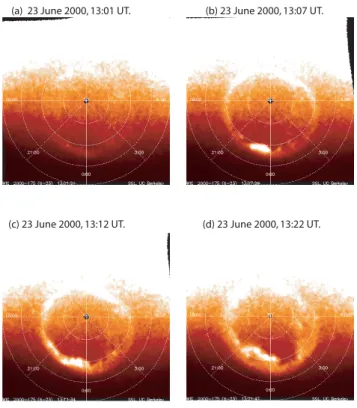
Fig. 3. Data from the Wideband Imaging Camera for the 23 June

2000. Figure 3a presents data from 13:01 UT, Fig. 3b presents data from 13:07 UT, Fig. 3c presents data from 13:12 UT and Fig. 3d presents data from 13:22 UT.

3 The statistical analysis

Mende et al. (2003) utilised the IMAGE FUV instrument to study the aurora in broad band using the WIC camera. They identified the onset time and the location (MLAT and MLT) of 113 substorms in 2000 and 2001, by a sudden brightening of the WIC images. Figure 3 presents WIC data from one of the substorm intervals identified by Mende et al. (2003), on 23 June 2000; this interval was included in the follow-ing statistical study. The figure presents data from 13:01 to 13:22 UT, where the auroral oval is clearly visible in all the plots. Substorm onset was identified at 13:07 UT. The plots clearly show an increase in auroral activity between 13:01 and 13:07 UT, with the signature of the onset of the substorm expansion phase.

One hundred and thirteen substorm intervals were iden-tified from the IMAGE FUV, with all the intervals in the years 2000 or 2001. During 67 of the intervals, the Su-perDARN radars were running in normal-resolution com-mon time mode (2-min resolution). For these 67 substorms we studied the l-o-s velocity measurements made by all the Northern Hemisphere SuperDARN radars, studying plasma flow from 30 min before substorm onset, until 30 min af-terwards. We aimed to perform a spatial superposed-epoch analysis of plasma flows during the substorm growth and ex-pansion phases. Initially, we mapped the l-o-s velocities ob-served by all the Northern Hemisphere radars during each substorm interval into the global grid defined by the

(5)

map-3610 G. Provan et al.: Statistical study of high-latitude plasma flow -800 -600 -400 -200 0 200 400 600 800 Velocity (m s -1 ) Ground Scatter Gridded l-o-s velocity data, 23 June 2000, 13:06 UT (Northern hemisphere) 12 MLT 18 MLT 6 MLT 24 MLT 60o 70o 80o FIG. 4

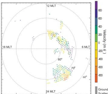
Fig. 4. Gridded line-of-sight velocity data from the SuperDARN

radars for 23 June 2000 at 13:06 UT.

potential analysis technique (Ruohoniemi and Baker, 1998). This global grid has grid cells which are 1◦in lat (∼111 km projected onto the Earth’s surface), and as close to 111 km in longitude as possible. This gridding system has the ad-vantage that it nearly equalizes cell areas, while the more conventional choice of a grid, defined by fixed steps in lat-itude and longlat-itude, has the disadvantage of a severe latitu-dinal variation in cell area. Figure 4 presents an example of the gridded l-o-s velocity data for one of the days included in the statistical study, on 23 June 2000, at 13:06 UT. The data are presented in a magnetic local time-magnetic latitude co-ordinate system in the Northern Hemisphere, with local midnight positioned at the bottom of each panel. During this interval there were data from all eight Northern Hemisphere SuperDARN radars available to us, except the Kodiak radar (radar A in Fig. 2).

Next, a substorm co-ordinate system was defined and each substorm interval was transformed in accordance with this co-ordinate system. The co-ordinate system defined points in terms of MLT and MLAT, where point (0,0) was the MLT and MLAT of the substorm onset, determined from the IM-AGE FUV data. For ease of data presentation the point (0,0) is chosen to be at a MLAT of 65◦and a MLT of midnight in the following figures. This position was chosen since 71% of the substorm onsets identified in the FUV data occurred within 90 min of midnight, and the average latitude of sub-storm onset was 65◦_{. We note that as 65}◦ _{is close to the}

equatorward edge of the SuperDARN field-of-view (in nor-mal scan mode), the substorm-affected region may only be partially imaged by the radars.

The actual co-ordinate transformation is best explained by an example. For the first substorm interval, on 23 June 2000,

the onset of the substorm expansion phase was identified at 13:07:17 UT, at a MLT of 23:00 and a MLAT of 69◦_{. Our}

first step involved gridding all the l-o-s velocity data for the period 12:37 to 13:37 UT, to the global grid described earlier. As the data has two-minute resolution, this represents 30 time samples. Next, for each of these 30 time samples, the loca-tions of all vectors were rotated in local time in accordance with the substorm co-ordinate system, with both the origin and the end point of the vectors being rotated. Thus, a vector previously positioned at 23:00 MLT, would be repositioned at 24:00 MLT. This is described by the below formula:

ϕ0=ϕ + α (1)

Where ϕ is the original longitude of the vectors’ start or end points, ϕ0is the new longitude of the flow vector and α is the angle of rotation. For this substorm α would be 15◦, equal to the angle of rotation needed to rotate the position of substorm onset to local midnight.

Next, for all 30 time samples the entire convection pattern would be stretched so that all points at 69:00 MLAT would be moved to 65.0 MLAT. All other points would be stretched in latitude by a factor that increased linearly, with increas-ing latitudinal separation from 90◦. This is defined by the formula below:

ø0=ø((90 − 65)/(90 − δs)) (2)

where ø is the co-latitude of the flow vector, ø0is the trans-formed co-latitude of the vector, and δsis the latitude of

sub-storm onset at subsub-storm onset, equal to 69◦for the this sub-storm.

This method of stretching the convection pattern was de-vised as a method of creating a global substorm co-ordinate system that would most closely maintain the original shape of the polar cap. Hereafter, all latitudes and local times will be referred to in relation to this substorm co-ordinate system. We transformed all 67 substorm intervals into the sub-storm co-ordinate system. We then combined the flow vec-tors from all of these substorms, considering each of the 30 time samples in turn. The 67 substorms together contained between 20 000 and 30 000 flow vectors at each of the 30 time samples. For each of the 30 time samples the l-o-s ve-locities were combined using a cosine fitting technique to find the best-fit flow vector. Originally, we intended to per-form the cosine fitting to the l-o-s velocities at each grid point. However, we realised that this resulted in such a large number of vectors that it was difficult to present them visu-ally. Instead, the cosine fitting technique was performed on all the l-o-s velocities observed within an area that covered 1 grid point in latitude (1 deg), and 2 grid points in longitude (approx. 220 km). Such cosine fitting was only performed if there was a minimum of five l-o-s velocity measurements within this area. Figure 5 presents an example of this cosine fitting technique, presenting the angle and velocity of the l-o-s velocities observed in the area extending from 70◦to 71◦ in latitude and from 0◦to 6◦in longitude, 30 min before sub-storm onset. Overplotted is a dashed line showing the l-o-s

(6)

G. Provan et al.: Statistical study of high-latitude plasma flow 3611 0 100 200 300 -2000 -1000 0 1000 2000 V elocit y (ms -1) Azimuthal angle

L-o-s velocities observed between the latitudes of 70o and 71o, and longitudes 0o to 6o 30 minutes before substorm onset. Overplottted is the cosine variation of the best-fit velocity.

Fig. 5. The velocity magnitude and azimuthal angle of l-o-s velocities observed by all the 67 substorms between 70◦and 71◦latitude and 0◦ and 6◦longitude at 30 min before substorm onset. The overplotted dashed line shows the cosine variation of the best-fit velocity.

velocity versus l-o-s angle for the best-fit flow vector. The velocity was calculated according to the formula below:

V = Vbestcos(α − αbest), (3)

where Vbest is the velocity of the best-fit flow, αbest is the

angle of the best-fit flow, V is the l-o-s velocity component and α is the magnetic azimuthal angle.

The end result is 30 convection maps of best-fit flow vec-tors representing the Northern Hemisphere global convection pattern every two minutes from 30 min before substorm on-set until 30 min afterwards. These maps were used as a basis to perform a detailed statistical study of high-latitude con-vection during the substorm growth and expansion phases. We were also able to determine estimates of cross polar-cap potential.

4 Results

4.1 IMF conditions

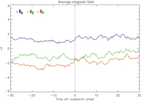
Before discussing the flows we present the upstream IMF conditions for the substorm intervals, from the ACE space-craft, to demonstrate the average background conditions. For each interval we calculated a delay between the time of the solar wind observation at ACE and the time it impinged at the dayside magnetopause, using the algorithm of Lester et al. (1993). The average IMF conditions (GSM) for all 67 substorm intervals are presented in Fig. 6. The plot shows that, on average the IMF Bx component is slightly positive,

while the average IMF Byand Bz components are negative.

From five minutes before substorm onset until onset itself the magnitude of the IMF Bzcomponent decreases (becomes

less negative), increasing by ∼1.5 nT.

4.2 Flow vectors

Figure 7 presents the cosine-fitted vectors at 10-min steps from 30 min prior to substorm onset (Fig. 7a) until substorm onset (Fig. 7d). Each plot includes data for a two-minute sample (the resolution of the radar data). The vectors are presented in what we term the substorm MLT/MLAT co-ordinate system described earlier, where the onset location is marked by a black cross on the plot. The velocity magni-tude is represented both by the length of the vector and by its colour, with blue representing the strongest flow and yellow the weakest. In Fig. 7a the flow presented is a two-cell con-vection pattern, with plasma flowing away from the Sun and across the polar cap at higher latitudes and returning at lower latitudes. Flows out of the polar cap on the nightside appear relatively weak. There is an asymmetry in the strength of the low-latitude sunward return flow, with stronger flows ob-served in the pre-midnight time sector compared to the post-midnight sector.

Figure 7b presents the cosine-fitted vectors 20 min before substorm onset. The high-latitude plasma flow into the po-lar cap on the dayside has now become stronger and more structured. There is still a dawn-dusk asymmetry in the strength of the sunward flow at lower latitude. The flows across the polar cap are also stronger than 10 min previously. Figure 7c presents the flow vectors 10 min before substorm onset. Strong flows into the polar cap are now observed be-tween ∼08:00 and ∼14:00 MLT. Compared to the flow vec-tors observed 30 min before substorm onset, the equatorward boundary of radar backscatter at midnight has moved from a latitude of 61◦to 59◦, the poleward boundary of midnight backscatter has also moved equatorward to a latitude of 82◦, from 84◦30 min before onset.

(7)

3612 G. Provan et al.: Statistical study of high-latitude plasma flow

- B

- Bx - B

- By - B

- Bz

Average magnetic field

Fig. 6. Average IMF conditions for all substorms. The IMF Bxcomponent is coloured blue, the Bycomponent is green and the Bzcomponent

is red.

Figure 7d presents the flow vectors at substorm onset. At the dayside the magnitude of the flow into the polar cap appears to have decreased compared to the flow observed 10 min before substorm onset, while the magnitude of the high-latitude plasma flowing out of the polar cap at the night-side has increased. There is an asymmetry in the strength of the nightside high-latitude plasma flowing out of the po-lar cap, with stronger flows observed in the pmidnight re-gion compared to the post-midnight rere-gion. The strength of the low-latitude return flow observed between ∼19:00 and

∼21:00 MLT has increased considerably. Between the MLTs of 21:00 and 24:00 we observe high velocity plasma flows out of the polar cap, travelling to lower latitudes. At a lati-tude of ∼70◦between 22:30 and 24:00 MLT, these fast flows appear to be stalled and diverted, travelling to lower latitudes at MLTs earlier than 22:30 and later than 24:00. Thus, there is evidence of a suppressed flow region on the nightside, cov-ering an area from approx 62◦_{to 70}◦_{latitude and from 22:30}

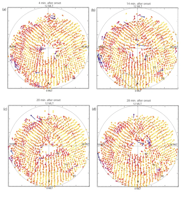
to 24:00 MLT, with fast flows diverted round its edges. Figure 8 presents the flow vectors 4 min after substorm on-set until 28 minutes after substorm onon-set. In Fig. 8a there are strong high-latitude flows out of the polar cap on the nightside. The nightside suppressed flow region observed at substorm onset is now more clearly defined, with enhanced plasma flow now being diverted to latitudes of 59◦ to 62◦, which is below this region of suppressed flow. There ap-pears to be stronger anti-sunward flows in the high-latitude dusk region as compared with the dawn region. The strong low-latitude return flow pmidnight of the auroral onset re-gion continues, with particularly strong flows observed in the post-dusk sector. Figure 8b presents the flow vectors 14 min after substorm onset. The flow pattern is very similar to the

flow pattern observed 4 min after substorm onset. The sup-pressed flow region is still clearly observable, although the strong flows at lower latitudes are somewhat reduced. In order to guide the eye, a dotted black circle marks the ap-proximate position of this region. Figure 8c presents the flow vectors observed 20 min after substorm onset. There is still strong plasma flow leaving the polar cap on the night-side, although this flow appears much less structured than the flow observed 14 min after the substorm onset. The night-side suppressed flow region appears to be further extended, stretching from approx. 60◦to 70◦MLAT, and from ∼22:00 to 02:30 MLT, with enhanced plasma flow being diverted around this region.

Figure 8d presents the flow vectors observed 28 min after substorm onset. The ionospheric flows are now much less structured than the flows observed 20 min after substorm on-set, but there is still strong plasma flow directed both into and out of the polar cap.

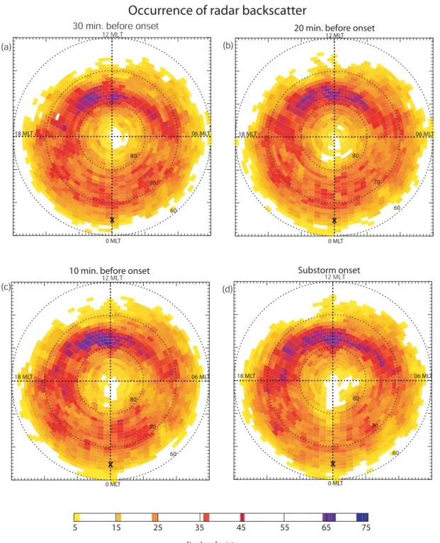
4.3 Backscatter occurrence

Figure 9 presents radar backscatter occurrence during the substorm growth phase, from 30 min before substorm onset (Fig. 9a) until substorm onset (Fig 9d), at intervals of 10 min. The plots shows how many Doppler velocity measurements have been used in the cosine fit to derive each vector in the flow plots. The occurrence is colour coded with blue rep-resenting the maximum number of points in the grid cell, and yellow the minimum. White represents less than 5 data points in the grid cell (note that the cosine fit is only per-formed if there is a minimum of 5 data points in a grid cell). During the growth phase there is little change in the oc-currence of radar backscatter. The greatest concentration of

(8)

30 min. before substorm onset

x x x x x x x x x x x x x x x x x x x x x x x x x x x x x x x x x x x x x x x x x x x x x x x x x x x x x x x x x x x x x x x x x x x x x x x x x x x x x x x x x x x x x x x x x x x x x x x x x x x x x x x x x x x x x x x x x x x x x x x x x x x x x x x x x x x x x x x x x x x x x x x x x x x x x x x x x x x x x x x x x x x x x x x x x x x x x x x x x x x x x x x x x x x x x x x x x x x x x x x x x x x x x x x x x x x x x x x x x x x x x x x x x x x x x x x x x x x x x x x x x x x x x x x x x x x x x x x x x x x x x x x x x x x x x x x x x x x x x x x x x x x x x x x x x x x x x x x x x x x x x x x x x x x x x x x x x x x x x x x x x x x x x x x x x x x x x x x x x x x x x x x x x x x x x x x x x x x x x x x x x x x x x x x x x x x x x x x x x x x x x x x x x x x x x x x x x x x x x x x x x x x x x x x x x x x x x x x x x x x x x x x x x x x x x x x x x x x x x x x x x x x x x x x x x x x x x x x x x x x x x x x x x x x x x x x x x x x x x x x x x x x x x x x x x x x x x x x x x x x x x x x x x x x x x x x x x x x x x x x x x x x x x x x x x x x x x x x x x x x x x x x x x x x x x x x x x x x x x x x x x x x x x x x x x x x x x x x x x x x x x x x x x x x x x x x x x x x x x x x x x x x x x x x x x x x x x x x x x x x x x x x x x x x x x x x x x x x x x x x x x x x x x x x x x x x x x x x x x x x x x x x x x x x x x x x x x x x x x x x x x x x x x x x x x x x x x x x x x x x x x x x x x x x x x x x x x x x x x x x x x x x x x x x x x x x x x x x x x x x x x x x x x x x x x x x x x x x x x x x x x x x x x x x x x x x x x x x x x x x x x x x x x x x x x x x x x x x x x x x x x x x x x x x x x x x x x x x x x x x x x x x x x x x x x x x x x x x x x x x x x x x x x x x x x x x x x x x x x x x x x x x x x x x x x x x x x x x x x x x x x x x x x x x x x x x x x x x x x x x x x x x x x x x x x x x x x x x x x x x x x x x x x x x x x x x x x x x x x x x x x x x x x x x x x x x x x x x x x x x x x x x x x x x x x x x x x x x x x x x x x x x x x x x x x x x x x x x x x x x x x x x x x x x x x x x x x x x x x x x x x x x x x x x x x x x x x x

x x x x x x x x x x x x x x x x x x x x x x x x x x x x x x x x x x x x x x x x x x x x x x x x x x x x x x x x x x x x x x x x x x x x x x x x x x x x x x x x x x x x x x x x x x x x x x x x x x x x x x x x x x x x x x x x x x x x x x x x x x x x x x x x x x x x x x x x x x x x x x x x x x x x x x x x x x x x x x x x x x x x x x x x x x x x x x x x x x x x x x x x x x x x x x x x x x x x x x x x x x x x x x x x x x x x x x x x x x x x x x x x x x x x x x x x x x x x x x x x x x x x x x x x x x x x x x x x x x x x x x x x x x x x x x x x x x x x x x x x x x x x x x x x x x x x x x x x x x x x x x x x x x x x x x x x x x x x x x x x x x x x x x x x x x x x x x x x x x x x x x x x x x x x x x x x x x x x x x x x x x x x x x x x x x x x x x x x x x x x x x x x x x x x x x x x x x x x x x x x x x x x x x x x x x x x x x x x x x x x x x x x x x x x x x x x x x x x x x x x x x x x x x x x x x x x x x x x x x x x x x x x x x x x x x x x x x x x x x x x x x x x x x x x x x x x x x x x x x x x x x x x x x x x x x x x x x x x x x x x x x x x x x x x x x x x x x x x x x x x x x x x x x x x x x x x x x x x x x x x x x x x x x x x x x x x x x x x x x x x x x x x x x x x x x x x x x x x x x x x x x x x x x x x x x x x x x x x x x x x x x x x x x x x x x x x x x x x x x x x x x x x x x x x x x x x x x x x x x x x x x x x x x x x x x x x x x x x x x x x x x x x x x x x x x x x x x x x x x x x x x x x x x x x x x x x x x x x x x x x x x x x x x x x x x x x x x x x x x x x x x x x x x x x x x x x x x x x x x x x x x x x x x x x x x x x x x x x x x x x x x x x x x x x x x x x x x x x x x x x x x x x x x x x x x x x x x x x x x x x x x x x x x x x x x x x x x x x x x x x x x x x x x x x x x x x x x x x x x x x x x x x x x x x x x x x x x x x x x x x x x x x x x x x x x x x x x x x x x x x x x x x x x x x x x x x x x x x x x x x x x x x x x x x x x x x x x x x x x x x x x x x x x x x x x x x x x x x x x x x x x x x x x x x x x x x x x x x x x x x x x x x x x x x x x x x x x x x x x x x x x x x x x x x x x x x x x x x x x x x x x x x x x x x x x x x x x x x x x x x x x x x x x x x x x x x x x x x x

x x x x x x x x x x x x x x x x x x x x x x x x x x x x x x x x x x x x x x x x x x x x x x x x x x x x x x x x x x x x x x x x x x x x x x x x x x x x x x x x x x x x x x x x x x x x x x x x x x x x x x x x x x x x x x x x x x x x x x x x x x x x x x x x x x x x x x x x x x x x x x x x x x x x x x x x x x x x x x x x x x x x x x x x x x x x x x x x x x x x x x x x x x x x x x x x x x x x x x x x x x x x x x x x x x x x x x x x x x x x x x x x x x x x x x x x x x x x x x x x x x x x x x x x x x x x x x x x x x x x x x x x x x x x x x x x x x x x x x x x x x x x x x x x x x x x x x x x x x x x x x x x x x x x x x x x x x x x x x x x x x x x x x x x x x x x x x x x x x x x x x x x x x x x x x x x x x x x x x x x x x x x x x x x x x x x x x x x x x x x x x x x x x x x x x x x x x x x x x x x x x x x x x x x x x x x x x x x x x x x x x x x x x x x x x x x x x x x x x x x x x x x x x x x x x x x x x x x x x x x x x x x x x x x x x x x x x x x x x x x x x x x x x x x x x x x x x x x x x x x x x x x x x x x x x x x x x x x x x x x x x x x x x x x x x x x x x x x x x x x x x x x x x x x x x x x x x x x x x x x x x x x x x x x x x x x x x x x x x x x x x x x x x x x x x x x x x x x x x x x x x x x x x x x x x x x x x x x x x x x x x x x x x x x x x x x x x x x x x x x x x x x x x x x x x x x x x x x x x x x x x x x x x x x x x x x x x x x x x x x x x x x x x x x x x x x x x x x x x x x x x x x x x x x x x x x x x x x x x x x x x x x x x x x x x x x x x x x x x x x x x x x x x x x x x x x x x x x x x x x x x x x x x x x x x x x x x x x x x x x x x x x x x x x x x x x x x x x x x x x x x x x x x x x x x x x x x x x x x x x x x x x x x x x x x x x x x x x x x x x x x x x x x x x x x x x x x x x x x x x x x x x x x x x x x x x x x x x x x x x x x x x x x x x x x x x x x x x x x x x x x x x x x x x x x x x x x x x x x x x x x x x x x x x x x x x x x x x x x x x x x x x x x x x x x x x x x x x x x x x x x x x x x x x x x x x x x x x x x x x x x x x x x x x x x x x x x x x x x x x x x x x x x x x x x x x x x x x x x x x x x x x x x x x x x x x x x x x x x x x x x x x x x x x x x x x x x x x x x x x x x x x x x x x x x x x x x x x x x x x x x

Northern hemisphere plasma flow vectors

0 m/s 200

400

600

800 1000

At substorm onset x x x x x x x x x x x x x x x x x x x x x x x x x x x x x x x x x x x x x x x x x x x x x x x x x x x x x x x x x x x x x x x x x x x x x x x x x x x x x x x x x x x x x x x x x x x x x x x x x x x x x x x x x x x x x x x x x x x x x x x x x x x x x x x x x x x x x x x x x x x x x x x x x x x x x x x x x x x x x x x x x x x x x x x x x x x x x x x x x x x x x x x x x x x x x x x x x x x x x x x x x x x x x x x x x x x x x x x x x x x x x x x x x x x x x x x x x x x x x x x x x x x x x x x x x x x x x x x x x x x x x x x x x x x x x x x x x x x x x x x x x x x x x x x x x x x x x x x x x x x x x x x x x x x x x x x x x x x x x x x x x x x x x x x x x x x x x x x x x x x x x x x x x x x x x x x x x x x x x x x x x x x x x x x x x x x x x x x x x x x x x x x x x x x x x x x x x x x x x x x x x x x x x x x x x x x x x x x x x x x x x x x x x x x x x x x x x x x x x x x x x x x x x x x x x x x x x x x x x x x x x x x x x x x x x x x x x x x x x x x x x x x x x x x x x x x x x x x x x x x x x x x x x x x x x x x x x x x x x x x x x x x x x x x x x x x x x x x x x x x x x x x x x x x x x x x x x x x x x x x x x x x x x x x x x x x x x x x x x x x x x x x x x x x x x x x x x x x x x x x x x x x x x x x x x x x x x x x x x x x x x x x x x x x x x x x x x x x x x x x x x x x x x x x x x x x x x x x x x x x x x x x x x x x x x x x x x x x x x x x x x x x x x x x x x x x x x x x x x x x x x x x x x x x x x x x x x x x x x x x x x x x x x x x x x x x x x x x x x x x x x x x x x x x x x x x x x x x x x x x x x x x x x x x x x x x x x x x x x x x x x x x x x x x x x x x x x x x x x x x x x x x x x x x x x x x x x x x x x x x x x x x x x x x x x x x x x x x x x x x x x x x x x x x x x x x x x x x x x x x x x x x x x x x x x x x x x x x x x x x x x x x x x x x x x x x x x x x x x x x x x x x x x x x x x x x x x x x x x x x x x x x x x x x x x x x x x x x x x x x x x x x x x x x x x x x x x x x x x x x x x x x x x x x x x x x x x x x x x x x x x x x x x x x x x x x x x x x x x x x x x x x x x x x x x x x x x x x x x x x x x x x x x x x x x x x x x x x x x x x x x x x x x x x x x x x x x x x x x x x x x x x x x x x 0 MLT 06 MLT 12 MLT 18 MLT 80 70 60 0 MLT 06 MLT 12 MLT 18 MLT 80 70 60 0 MLT 06 MLT 12 MLT 18 MLT 80 70 60 0 MLT 06 MLT 12 MLT 18 MLT 80 70 60 (a) (b) (c) (d)

Fig. 7. Cosine-fitted velocity flow vectors at 10-min steps from 30 min prior to substorm onset (Fig. 7a) until substorm onset (Fig. 7d). The

velocity magnitude is represented both by the length of the vector and by its colour, with blue representing the strongest flow and yellow the weakest.

radar backscatter is centred at the dayside. There is a slight dawn/dusk asymmetry in the occurrence of data points be-tween the latitude of 65◦to 80◦, with more points being ob-served in the dusk region as compared to the dawn region. Figure 9d presents the radar backscatter at substorm onset. Nightside backscatter has moved equatorward. There is a clear change in the occurrence plots compared to the growth phase, with a decline in the amount of backscatter in the mid-night region, although the occurrence of backscatter in the midday region remains the same.

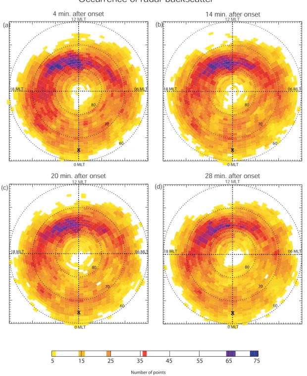
Figure 10 presents the occurrence of radar backscatter dur-ing the substorm expansion phase, from four minutes after substorm expansion phase onset (Fig. 10a) until 28 min after substorm expansion phase onset (Fig. 10d). In Fig. 10a the greatest concentration of backscatter occurrence is clearly skewed to the post-noon sector, observed at magnetic latitude of approx. 64◦to 70◦and MLT of 12:00 to 16:00. This asym-metry of radar backscatter can be observed during the entire expansion phase. As the expansion phase develops there is a decreasing amount of nightside backscatter, eventually

(9)

af-3614 G. Provan et al.: Statistical study of high-latitude plasma flow

4 min. after onset

x x x x x x x x x x x x x x x x x x x x x x x x x x x x x x x x x x x x x x x x x x x x x x x x x x x x x x x x x x x x x x x x x x x x x x x x x x x x x x x x x x x x x x x x x x x x x x x x x x x x x x x x x x x x x x x x x x x x x x x x x x x x x x x x x x x x x x x x x x x x x x x x x x x x x x x x x x x x x x x x x x x x x x x x x x x x x x x x x x x x x x x x x x x x x x x x x x x x x x x x x x x x x x x x x x x x x x x x x x x x x x x x x x x x x x x x x x x x x x x x x x x x x x x x x x x x x x x x x x x x x x x x x x x x x x x x x x x x x x x x x x x x x x x x x x x x x x x x x x x x x x x x x x x x x x x x x x x x x x x x x x x x x x x x x x x x x x x x x x x x x x x x x x x x x x x x x x x x x x x x x x x x x x x x x x x x x x x x x x x x x x x x x x x x x x x x x x x x x x x x x x x x x x x x x x x x x x x x x x x x x x x x x x x x x x x x x x x x x x x x x x x x x x x x x x x x x x x x x x x x x x x x x x x x x x x x x x x x x x x x x x x x x x x x x x x x x x x x x x x x x x x x x x x x x x x x x x x x x x x x x x x x x x x x x x x x x x x x x x x x x x x x x x x x x x x x x x x x x x x x x x x x x x x x x x x x x x x x x x x x x x x x x x x x x x x x x x x x x x x x x x x x x x x x x x x x x x x x x x x x x x x x x x x x x x x x x x x x x x x x x x x x x x x x x x x x x x x x x x x x x x x x x x x x x x x x x x x x x x x x x x x x x x x x x x x x x x x x x x x x x x x x x x x x x x x x x x x x x x x x x x x x x x x x x x x x x x x x x x x x x x x x x x x x x x x x x x x x x x x x x x x x x x x x x x x x x x x x x x x x x x x x x x x x x x x x x x x x x x x x x x x x x x x x x x x x x x x x x x x x x x x x x x x x x x x x x x x x x x x x x x x x x x x x x x x x x x x x x x x x x x x x x x x x x x x x x x x x x x x x x x x x x x x x x x x x x x x x x x x x x x x x x x x x x x x x x x x x x x x x x x x x x x x x x x x x x x x x x x x x x x x x x x x x x x x x x x x x x x x x x x x x x x x x x x x x x x x x x x x x x x x x x x x x x x x x x x x x x x x x x x x x x x x x x x x x x x x x x x x x x x x x x x x x x x x x x x x x x x x x x x x x x x x x x x x x x x x x x x x x x x x x x x x 0 MLT 06 MLT 12 MLT 18 MLT 80 70 60

14 min. after onset

x x x x x x x x x x x x x x x x x x x x x x x x x x x x x x x x x x x x x x x x x x x x x x x x x x x x x x x x x x x x x x x x x x x x x x x x x x x x x x x x x x x x x x x x x x x x x x x x x x x x x x x x x x x x x x x x x x x x x x x x x x x x x x x x x x x x x x x x x x x x x x x x x x x x x x x x x x x x x x x x x x x x x x x x x x x x x x x x x x x x x x x x x x x x x x x x x x x x x x x x x x x x x x x x x x x x x x x x x x x x x x x x x x x x x x x x x x x x x x x x x x x x x x x x x x x x x x x x x x x x x x x x x x x x x x x x x x x x x x x x x x x x x x x x x x x x x x x x x x x x x x x x x x x x x x x x x x x x x x x x x x x x x x x x x x x x x x x x x x x x x x x x x x x x x x x x x x x x x x x x x x x x x x x x x x x x x x x x x x x x x x x x x x x x x x x x x x x x x x x x x x x x x x x x x x x x x x x x x x x x x x x x x x x x x x x x x x x x x x x x x x x x x x x x x x x x x x x x x x x x x x x x x x x x x x x x x x x x x x x x x x x x x x x x x x x x x x x x x x x x x x x x x x x x x x x x x x x x x x x x x x x x x x x x x x x x x x x x x x x x x x x x x x x x x x x x x x x x x x x x x x x x x x x x x x x x x x x x x x x x x x x x x x x x x x x x x x x x x x x x x x x x x x x x x x x x x x x x x x x x x x x x x x x x x x x x x x x x x x x x x x x x x x x x x x x x x x x x x x x x x x x x x x x x x x x x x x x x x x x x x x x x x x x x x x x x x x x x x x x x x x x x x x x x x x x x x x x x x x x x x x x x x x x x x x x x x x x x x x x x x x x x x x x x x x x x x x x x x x x x x x x x x x x x x x x x x x x x x x x x x x x x x x x x x x x x x x x x x x x x x x x x x x x x x x x x x x x x x x x x x x x x x x x x x x x x x x x x x x x x x x x x x x x x x x x x x x x x x x x x x x x x x x x x x x x x x x x x x x x x x x x x x x x x x x x x x x x x x x x x x x x x x x x x x x x x x x x x x x x x x x x x x x x x x x x x x x x x x x x x x x x x x x x x x x x x x x x x x x x x x x x x x x x x x x x x x x x x x x x x x x x x x x x x x x x x x x x x x x x x x x x x x x x x x x x x x x x x x x x x x x x x x x x x x x x x x x x x x x x x x x x x x x x x x x x x x x x x x x x x x x x x x x x x x x x x x x x x x x x x x

20 min. after onset

x x x x x x x x x x x x x x x x x x x x x x x x x x x x x x x x x x x x x x x x x x x x x x x x x x x x x x x x x x x x x x x x x x x x x x x x x x x x x x x x x x x x x x x x x x x x x x x x x x x x x x x x x x x x x x x x x x x x x x x x x x x x x x x x x x x x x x x x x x x x x x x x x x x x x x x x x x x x x x x x x x x x x x x x x x x x x x x x x x x x x x x x x x x x x x x x x x x x x x x x x x x x x x x x x x x x x x x x x x x x x x x x x x x x x x x x x x x x x x x x x x x x x x x x x x x x x x x x x x x x x x x x x x x x x x x x x x x x x x x x x x x x x x x x x x x x x x x x x x x x x x x x x x x x x x x x x x x x x x x x x x x x x x x x x x x x x x x x x x x x x x x x x x x x x x x x x x x x x x x x x x x x x x x x x x x x x x x x x x x x x x x x x x x x x x x x x x x x x x x x x x x x x x x x x x x x x x x x x x x x x x x x x x x x x x x x x x x x x x x x x x x x x x x x x x x x x x x x x x x x x x x x x x x x x x x x x x x x x x x x x x x x x x x x x x x x x x x x x x x x x x x x x x x x x x x x x x x x x x x x x x x x x x x x x x x x x x x x x x x x x x x x x x x x x x x x x x x x x x x x x x x x x x x x x x x x x x x x x x x x x x x x x x x x x x x x x x x x x x x x x x x x x x x x x x x x x x x x x x x x x x x x x x x x x x x x x x x x x x x x x x x x x x x x x x x x x x x x x x x x x x x x x x x x x x x x x x x x x x x x x x x x x x x x x x x x x x x x x x x x x x x x x x x x x x x x x x x x x x x x x x x x x x x x x x x x x x x x x x x x x x x x x x x x x x x x x x x x x x x x x x x x x x x x x x x x x x x x x x x x x x x x x x x x x x x x x x x x x x x x x x x x x x x x x x x x x x x x x x x x x x x x x x x x x x x x x x x x x x x x x x x x x x x x x x x x x x x x x x x x x x x x x x x x x x x x x x x x x x x x x x x x x x x x x x x x x x x x x x x x x x x x x x x x x x x x x x x x x x x x x x x x x x x x x x x x x x x x x x x x x x x x x x x x x x x x x x x x x x x x x x x x x x x x x x x x x x x x x x x x x x x x x x x x x x x x x x x x x x x x x x x x x x x x x x x x x x x x x x x x x x x x x x x x x x x x x x x x x x x x x x x x x x x x x x x x x x x x x x x x x x x x x x x x x x x x x x x x x x x x x x x x x x

28 min. after onset

x x x x x x x x x x x x x x x x x x x x x x x x x x x x x x x x x x x x x x x x x x x x x x x x x x x x x x x x x x x x x x x x x x x x x x x x x x x x x x x x x x x x x x x x x x x x x x x x x x x x x x x x x x x x x x x x x x x x x x x x x x x x x x x x x x x x x x x x x x x x x x x x x x x x x x x x x x x x x x x x x x x x x x x x x x x x x x x x x x x x x x x x x x x x x x x x x x x x x x x x x x x x x x x x x x x x x x x x x x x x x x x x x x x x x x x x x x x x x x x x x x x x x x x x x x x x x x x x x x x x x x x x x x x x x x x x x x x x x x x x x x x x x x x x x x x x x x x x x x x x x x x x x x x x x x x x x x x x x x x x x x x x x x x x x x x x x x x x x x x x x x x x x x x x x x x x x x x x x x x x x x x x x x x x x x x x x x x x x x x x x x x x x x x x x x x x x x x x x x x x x x x x x x x x x x x x x x x x x x x x x x x x x x x x x x x x x x x x x x x x x x x x x x x x x x x x x x x x x x x x x x x x x x x x x x x x x x x x x x x x x x x x x x x x x x x x x x x x x x x x x x x x x x x x x x x x x x x x x x x x x x x x x x x x x x x x x x x x x x x x x x x x x x x x x x x x x x x x x x x x x x x x x x x x x x x x x x x x x x x x x x x x x x x x x x x x x x x x x x x x x x x x x x x x x x x x x x x x x x x x x x x x x x x x x x x x x x x x x x x x x x x x x x x x x x x x x x x x x x x x x x x x x x x x x x x x x x x x x x x x x x x x x x x x x x x x x x x x x x x x x x x x x x x x x x x x x x x x x x x x x x x x x x x x x x x x x x x x x x x x x x x x x x x x x x x x x x x x x x x x x x x x x x x x x x x x x x x x x x x x x x x x x x x x x x x x x x x x x x x x x x x x x x x x x x x x x x x x x x x x x x x x x x x x x x x x x x x x x x x x x x x x x x x x x x x x x x x x x x x x x x x x x x x x x x x x x x x x x x x x x x x x x x x x x x x x x x x x x x x x x x x x x x x x x x x x x x x x x x x x x x x x x x x x x x x x x x x x x x x x x x x x x x x x x x x x x x x x x x x x x x x x x x x x x x x x x x x x x x x x x x x x x x x x x x x x x x x x x x x x x x x x x x x x x x x x x x x x x x x x x x x x x x x x x x x x x x x x x x x x x x x x x x x x x x x x x x x x x x x x x x x x x x x x x x

0 m/s 200

400

600

800 1000

Northern hemisphere plasma flow vectors

0 MLT 06 MLT 12 MLT 18 MLT 80 70 60 0 MLT 06 MLT 12 MLT 18 MLT 80 70 60 0 MLT 06 MLT 12 MLT 18 MLT 80 70 60 (a) _(b) (c) (d)

Fig. 8. Cosine-fitted velocity flow vectors presented from 4 min after substorm onset (Fig. 8a) until 28 min after substorm onset (Fig. 8d).

The velocity magnitude is represented both by the length of the vector and by its colour, with blue representing the strongest flow and yellow the weakest. In Fig. 8b a dotted black circle marks the approximate position of the suppressed flow region.

fecting almost the entire nightside region from dusk to dawn. However, the occurrence of radar backscatter in the dayside region only shows a small decline.

4.4 Polar cap velocities

The cosine-fitted vectors were used to derive the mean ve-locities across the entire polar cap, and across the dawn and

dusk sectors of the polar cap. The flow reversal boundary was considered a proxy for the polar cap boundary. The first step was to measure the width of the polar cap across the dawn-dusk meridian, measured from the position of flow reversal in the dawn sector to the position of flow reversal in the dusk sector. This measurement was taken as a proxy for the width of the polar cap. We then calculated the mean anti-sunward velocity across the dawn-dusk meridian, and also separately

(10)

30 min. before onset

xxxxxxxxxxxxxxxxxxxxxxxxxxxxxxxxxxxxxxxxxxxxxxxxxxxxxxxxxxxxxxxxxxxxxxxxxxxxxxxxxxxxxxxxxxxxxxxxxxxxxxxxxxxxxxxxxxxxxxxxxxxxxxxxxxxxxxxxxxxxxxxxxxxxxxxxxxxxxxxxxxxxxxxxxxxxxxxxxxxxxxxxxxxxxxxxxxxxxxxxxxxxxxxxxxxxxxxxxxxxxxxxxxxxxxxxxxxxxxxxxxxxxxxxxxxxxxxxxxxxxxxxxxxxxxxxxxxxxxxxxxxxxxxxxxxxxxxxxxxxxxxxxxxxxxxxxxxxxxxxxxxxxxxxxxxxxxxxxxxxxxxxxxxxxxxxxxxxxxxxxxxxxxxxxxxxxxxxxxxxxxxxxxxxxxxxxxxxxxxxxxxxxxxxxxxxxxxxxxxxxxxxxxxxxxxxxxxxxxxxxxxxxxxxxxxxxxxxxxxxxxxxxxxxxxxxxxxxxxxxxxxxxxxxxxxxxxxxxxxxxxxxxxxxxxxxxxxxxxxxxxxxxxxxxxxxxxxxxxxxxxxxxxxxxxxxxxxxxxxxxxxxxxxxxxxxxxxxxxxxxxxxxxxxxxxxxxxxxxxxxxxxxxxxxxxxxxxxxxxxxxxxxxxxxxxxxxxxxxxxxxxxxxxxxxxxxxxxxxxxxxxxxxxxxxxxxxxxxxxxxxxxxxxxxxxxxxxxxxxxxxxxxxxxxxxxxxxxxxxxxxxxxxxxxxxxxxxxxxxxxxxxxxxxxxxxxxxxxxxxxxxxxxxxxxxxxxxxxxxxxxxxxxxxxxxxxxxxxxxxxxxxxxxxxxxxxxxxxxxxxxxxxxxxxxxxxxxxxxxxxxxxxxxxxxxxxxxxxxxxxxxxxxxxxxxxxxxxxxxxxxxxxxxxxxxxxxxxxxxxxxxxxxxxxxxxxxxxxxxxxxxxxxxxxxxxxxxxxxxxxxxxxxxxxxxxxxxxxxxxxxxxxxxxxxxxxxxxxxxxxxxxxxxxxxxxxxxxxxxxxxxxxxxxxxxxxxxxxxxxxxxxxxxxxxxxxx 0 MLT 06 MLT 12 MLT 18 MLT 80 70 60

xxxxxxxxxxxxxxxxxxxxxxxxxxxxxxxxxxxxxxxxxxxxxxxxxxxxxxxxxxxxxxxxxxxxxxxxxxxxxxxxxxxxxxxxxxxxxxxxxxxxxxxxxxxxxxxxxxxxxxxxxxxxxxxxxxxxxxxxxxxxxxxxxxxxxxxxxxxxxxxxxxxxxxxxxxxxxxxxxxxxxxxxxxxxxxxxxxxxxxxxxxxxxxxxxxxxxxxxxxxxxxxxxxxxxxxxxxxxxxxxxxxxxxxxxxxxxxxxxxxxxxxxxxxxxxxxxxxxxxxxxxxxxxxxxxxxxxxxxxxxxxxxxxxxxxxxxxxxxxxxxxxxxxxxxxxxxxxxxxxxxxxxxxxxxxxxxxxxxxxxxxxxxxxxxxxxxxxxxxxxxxxxxxxxxxxxxxxxxxxxxxxxxxxxxxxxxxxxxxxxxxxxxxxxxxxxxxxxxxxxxxxxxxxxxxxxxxxxxxxxxxxxxxxxxxxxxxxxxxxxxxxxxxxxxxxxxxxxxxxxxxxxxxxxxxxxxxxxxxxxxxxxxxxxxxxxxxxxxxxxxxxxxxxxxxxxxxxxxxxxxxxxxxxxxxxxxxxxxxxxxxxxxxxxxxxxxxxxxxxxxxxxxxxxxxxxxxxxxxxxxxxxxxxxxxxxxxxxxxxxxxxxxxxxxxxxxxxxxxxxxxxxxxxxxxxxxxxxxxxxxxxxxxxxxxxxxxxxxxxxxxxxxxxxxxxxxxxxxxxxxxxxxxxxxxxxxxxxxxxxxxxxxxxxxxxxxxxxxxxxxxxxxxxxxxxxxxxxxxxxxxxxxxxxxxxxxxxxxxxxxxxxxxxxxxxxxxxxxxxxxxxxxxxxxxxxxxxxxxxxxxxxxxxxxxxxxxxxxxxxxxxxxxxxxxxxxxxxxxxxxxxxxxxxxxxxxxxxxxxxxxxxxxxxxxxxxxxxxxxxxxxxxxxxxxxxxxxxxxxxxxxxxxxxxxxxxxxxxxxxxxxxxxxxxxxxxxxxxxxxxxxxxxxxxxxxxxxxxxxxxxxxxxxxxxxxxxxxxxxxxxxxxxxxxxxxxxxxxxxxxxxxxxxxxxxxxxxxx 0 MLT 06 MLT 12 MLT 18 MLT 80 70 60

xxxxxxxxxxxxxxxxxxxxxxxxxxxxxxxxxxxxxxxxxxxxxxxxxxxxxxxxxxxxxxxxxxxxxxxxxxxxxxxxxxxxxxxxxxxxxxxxxxxxxxxxxxxxxxxxxxxxxxxxxxxxxxxxxxxxxxxxxxxxxxxxxxxxxxxxxxxxxxxxxxxxxxxxxxxxxxxxxxxxxxxxxxxxxxxxxxxxxxxxxxxxxxxxxxxxxxxxxxxxxxxxxxxxxxxxxxxxxxxxxxxxxxxxxxxxxxxxxxxxxxxxxxxxxxxxxxxxxxxxxxxxxxxxxxxxxxxxxxxxxxxxxxxxxxxxxxxxxxxxxxxxxxxxxxxxxxxxxxxxxxxxxxxxxxxxxxxxxxxxxxxxxxxxxxxxxxxxxxxxxxxxxxxxxxxxxxxxxxxxxxxxxxxxxxxxxxxxxxxxxxxxxxxxxxxxxxxxxxxxxxxxxxxxxxxxxxxxxxxxxxxxxxxxxxxxxxxxxxxxxxxxxxxxxxxxxxxxxxxxxxxxxxxxxxxxxxxxxxxxxxxxxxxxxxxxxxxxxxxxxxxxxxxxxxxxxxxxxxxxxxxxxxxxxxxxxxxxxxxxxxxxxxxxxxxxxxxxxxxxxxxxxxxxxxxxxxxxxxxxxxxxxxxxxxxxxxxxxxxxxxxxxxxxxxxxxxxxxxxxxxxxxxxxxxxxxxxxxxxxxxxxxxxxxxxxxxxxxxxxxxxxxxxxxxxxxxxxxxxxxxxxxxxxxxxxxxxxxxxxxxxxxxxxxxxxxxxxxxxxxxxxxxxxxxxxxxxxxxxxxxxxxxxxxxxxxxxxxxxxxxxxxxxxxxxxxxxxxxxxxxxxxxxxxxxxxxxxxxxxxxxxxxxxxxxxxxxxxxxxxxxxxxxxxxxxxxxxxxxxxxxxxxxxxxxxxxxxxxxxxxxxxxxxxxxxxxxxxxxxxxxxxxxxxxxxxxxxxxxxxxxxxxxxxxxxxxxxxxxxxxxxxxxxxxxxxxxxxxxxxxxxxxxxxxxxxxxxxxxxxxxxxxxxxxxxxxxxxxxxxxxxxxxxxxxxxxxxxxxxxxxxxxxxxxxxxxxxxxxxxxxxxxxxx 0 MLT 06 MLT 12 MLT 18 MLT 80 70 60 Substorm onset xxxxxxxxxxxxxxxxxxxxxxxxxxxxxxxxxxxxxxxxxxxxxxxxxxxxxxxxxxxxxxxxxxxxxxxxxxxxxxxxxxxxxxxxxxxxxxxxxxxxxxxxxxxxxxxxxxxxxxxxxxxxxxxxxxxxxxxxxxxxxxxxxxxxxxxxxxxxxxxxxxxxxxxxxxxxxxxxxxxxxxxxxxxxxxxxxxxxxxxxxxxxxxxxxxxxxxxxxxxxxxxxxxxxxxxxxxxxxxxxxxxxxxxxxxxxxxxxxxxxxxxxxxxxxxxxxxxxxxxxxxxxxxxxxxxxxxxxxxxxxxxxxxxxxxxxxxxxxxxxxxxxxxxxxxxxxxxxxxxxxxxxxxxxxxxxxxxxxxxxxxxxxxxxxxxxxxxxxxxxxxxxxxxxxxxxxxxxxxxxxxxxxxxxxxxxxxxxxxxxxxxxxxxxxxxxxxxxxxxxxxxxxxxxxxxxxxxxxxxxxxxxxxxxxxxxxxxxxxxxxxxxxxxxxxxxxxxxxxxxxxxxxxxxxxxxxxxxxxxxxxxxxxxxxxxxxxxxxxxxxxxxxxxxxxxxxxxxxxxxxxxxxxxxxxxxxxxxxxxxxxxxxxxxxxxxxxxxxxxxxxxxxxxxxxxxxxxxxxxxxxxxxxxxxxxxxxxxxxxxxxxxxxxxxxxxxxxxxxxxxxxxxxxxxxxxxxxxxxxxxxxxxxxxxxxxxxxxxxxxxxxxxxxxxxxxxxxxxxxxxxxxxxxxxxxxxxxxxxxxxxxxxxxxxxxxxxxxxxxxxxxxxxxxxxxxxxxxxxxxxxxxxxxxxxxxxxxxxxxxxxxxxxxxxxxxxxxxxxxxxxxxxxxxxxxxxxxxxxxxxxxxxxxxxxxxxxxxxxxxxxxxxxxxxxxxxxxxxxxxxxxxxxxxxxxxxxxxxxxxxxxxxxxxxxxxxxxxxxxxxxxxxxxxxxxxxxxxxxxxxxxxxxxxxxxxxxxxxxxxxxxxxxxxxxxxxxxxxxxxxxxxxxxxxxxxxxxxxxxxxxxxxxxxxxxxxxxxxxxxxxxxxxxxxxxxxxxxxxxxxxxxxxxxxxxx 0 MLT 06 MLT 12 MLT 18 MLT 80 70 60 Number of points 5 15 25 35 45 55 65 75

Occurrence of radar backscatter

(a) (b)

(c) _(d)

Fig. 9. Radar backscatter occurrence from 30 min before substorm onset (Fig. 9a) until substorm onset (Fig. 9d). The occurrence is colour

coded with blue representing the maximum number of points and yellow the minimum. White represents less than 5 data points.

across the dawn and dusk regions. This velocity was derived by averaging all cosine-fitted vectors along the dawn-dusk meridian for each time sector. As each cosine-fitted vector is derived from a number of vectors itself, the mean velocity was weighted by the number of l-o-s velocities used to esti-mate each cosine-fitted vector. So, for the example presented in Fig. 5, this cosine-fitted velocity would have a weight of 34. Figure 11 presents the anti-sunward component of the average flow velocity across the dawn (blue line) and dusk

(red line) sectors of the polar cap and across the entire polar cap (black line). Each velocity has an error bar associated with it, which is the standard error of the weighted mean. At each time sample we performed a student t-test in order to investigate whether the difference in the weighted mean be-tween the dawn and the dusk sectors was significant at the 95% confidence level. If the difference in velocity was sig-nificant, the dawn and dusk velocities were marked with a cross. There are only 9 time samples, out of the 30, that

(11)

3616 G. Provan et al.: Statistical study of high-latitude plasma flow xxxxxxxxxxxxxxxxxxxxxxxxxxxxxxxxxxxxxxxxxxxxxxxxxxxxxxxxxxxxxxxxxxxxxxxxxxxxxxxxxxxxxxxxxxxxxxxxxxxxxxxxxxxxxxxxxxxxxxxxxxxxxxxxxxxxxxxxxxxxxxxxxxxxxxxxxxxxxxxxxxxxxxxxxxxxxxxxxxxxxxxxxxxxxxxxxxxxxxxxxxxxxxxxxxxxxxxxxxxxxxxxxxxxxxxxxxxxxxxxxxxxxxxxxxxxxxxxxxxxxxxxxxxxxxxxxxxxxxxxxxxxxxxxxxxxxxxxxxxxxxxxxxxxxxxxxxxxxxxxxxxxxxxxxxxxxxxxxxxxxxxxxxxxxxxxxxxxxxxxxxxxxxxxxxxxxxxxxxxxxxxxxxxxxxxxxxxxxxxxxxxxxxxxxxxxxxxxxxxxxxxxxxxxxxxxxxxxxxxxxxxxxxxxxxxxxxxxxxxxxxxxxxxxxxxxxxxxxxxxxxxxxxxxxxxxxxxxxxxxxxxxxxxxxxxxxxxxxxxxxxxxxxxxxxxxxxxxxxxxxxxxxxxxxxxxxxxxxxxxxxxxxxxxxxxxxxxxxxxxxxxxxxxxxxxxxxxxxxxxxxxxxxxxxxxxxxxxxxxxxxxxxxxxxxxxxxxxxxxxxxxxxxxxxxxxxxxxxxxxxxxxxxxxxxxxxxxxxxxxxxxxxxxxxxxxxxxxxxxxxxxxxxxxxxxxxxxxxxxxxxxxxxxxxxxxxxxxxxxxxxxxxxxxxxxxxxxxxxxxxxxxxxxxxxxxxxxxxxxxxxxxxxxxxxxxxxxxxxxxxxxxxxxxxxxxxxxxxxxxxxxxxxxxxxxxxxxxxxxxxxxxxxxxxxxxxxxxxxxxxxxxxxxxxxxxxxxxxxxxxxxxxxxxxxxxxxxxxxxxxxxxxxxxxxxxxxxxxxxxxxxxxxxxxxxxxxxxxxxxxxxxxxxxxxxxxxxxxxxxxxxxxxxxxxxxxxxxxxxxxxxxxxxxxxxxxxxxxxxxxxxxxxxxxxxxxxxxxxxxxxxxxxxxxxxxxxxxxxxxxxxxxxxxxxxxxxxxxxxxxxxxxxx xxxxxxxxxxxxxxxxxxxxxxxxxxxxxxxxxxxxxxxxxxxxxxxxxxxxxxxxxxxxxxxxxxxxxxxxxxxxxxxxxxxxxxxxxxxxxxxxxxxxxxxxxxxxxxxxxxxxxxxxxxxxxxxxxxxxxxxxxxxxxxxxxxxxxxxxxxxxxxxxxxxxxxxxxxxxxxxxxxxxxxxxxxxxxxxxxxxxxxxxxxxxxxxxxxxxxxxxxxxxxxxxxxxxxxxxxxxxxxxxxxxxxxxxxxxxxxxxxxxxxxxxxxxxxxxxxxxxxxxxxxxxxxxxxxxxxxxxxxxxxxxxxxxxxxxxxxxxxxxxxxxxxxxxxxxxxxxxxxxxxxxxxxxxxxxxxxxxxxxxxxxxxxxxxxxxxxxxxxxxxxxxxxxxxxxxxxxxxxxxxxxxxxxxxxxxxxxxxxxxxxxxxxxxxxxxxxxxxxxxxxxxxxxxxxxxxxxxxxxxxxxxxxxxxxxxxxxxxxxxxxxxxxxxxxxxxxxxxxxxxxxxxxxxxxxxxxxxxxxxxxxxxxxxxxxxxxxxxxxxxxxxxxxxxxxxxxxxxxxxxxxxxxxxxxxxxxxxxxxxxxxxxxxxxxxxxxxxxxxxxxxxxxxxxxxxxxxxxxxxxxxxxxxxxxxxxxxxxxxxxxxxxxxxxxxxxxxxxxxxxxxxxxxxxxxxxxxxxxxxxxxxxxxxxxxxxxxxxxxxxxxxxxxxxxxxxxxxxxxxxxxxxxxxxxxxxxxxxxxxxxxxxxxxxxxxxxxxxxxxxxxxxxxxxxxxxxxxxxxxxxxxxxxxxxxxxxxxxxxxxxxxxxxxxxxxxxxxxxxxxxxxxxxxxxxxxxxxxxxxxxxxxxxxxxxxxxxxxxxxxxxxxxxxxxxxxxxxxxxxxxxxxxxxxxxxxxxxxxxxxxxxxxxxxxxxxxxxxxxxxxxxxxxxxxxxxxxxxxxxxxxxxxxxxxxxxxxxxxxxxxxxxxxxxxxxxxxxxxxxxxxxxxxxxxxxxxxxxxxxxxxxxxxxxxxxxxxxxxxxxxxxxxxxxxxxxxxxxxxxxxxxxxxxxxxxxxxxxxxxxxxxx xxxxxxxxxxxxxxxxxxxxxxxxxxxxxxxxxxxxxxxxxxxxxxxxxxxxxxxxxxxxxxxxxxxxxxxxxxxxxxxxxxxxxxxxxxxxxxxxxxxxxxxxxxxxxxxxxxxxxxxxxxxxxxxxxxxxxxxxxxxxxxxxxxxxxxxxxxxxxxxxxxxxxxxxxxxxxxxxxxxxxxxxxxxxxxxxxxxxxxxxxxxxxxxxxxxxxxxxxxxxxxxxxxxxxxxxxxxxxxxxxxxxxxxxxxxxxxxxxxxxxxxxxxxxxxxxxxxxxxxxxxxxxxxxxxxxxxxxxxxxxxxxxxxxxxxxxxxxxxxxxxxxxxxxxxxxxxxxxxxxxxxxxxxxxxxxxxxxxxxxxxxxxxxxxxxxxxxxxxxxxxxxxxxxxxxxxxxxxxxxxxxxxxxxxxxxxxxxxxxxxxxxxxxxxxxxxxxxxxxxxxxxxxxxxxxxxxxxxxxxxxxxxxxxxxxxxxxxxxxxxxxxxxxxxxxxxxxxxxxxxxxxxxxxxxxxxxxxxxxxxxxxxxxxxxxxxxxxxxxxxxxxxxxxxxxxxxxxxxxxxxxxxxxxxxxxxxxxxxxxxxxxxxxxxxxxxxxxxxxxxxxxxxxxxxxxxxxxxxxxxxxxxxxxxxxxxxxxxxxxxxxxxxxxxxxxxxxxxxxxxxxxxxxxxxxxxxxxxxxxxxxxxxxxxxxxxxxxxxxxxxxxxxxxxxxxxxxxxxxxxxxxxxxxxxxxxxxxxxxxxxxxxxxxxxxxxxxxxxxxxxxxxxxxxxxxxxxxxxxxxxxxxxxxxxxxxxxxxxxxxxxxxxxxxxxxxxxxxxxxxxxxxxxxxxxxxxxxxxxxxxxxxxxxxxxxxxxxxxxxxxxxxxxxxxxxxxxxxxxxxxxxxxxxxxxxxxxxxxxxxxxxxxxxxxxxxxxxxxxxxxxxxxxxxxxxxxxxxxxxxxxxxxxxxxxxxxxxxxxxxxxxxxxxxxxxxxxxxxxxxxxxxxxxxxxxxxxxxxxxxxxxxxxxxxxxxxxxxxxxxxxxxxxxxxxxxxxxxxxxxxxxxxxxxxxxxxxxxxxxxxxxxxxxxxxxxxxxxx xxxxxxxxxxxxxxxxxxxxxxxxxxxxxxxxxxxxxxxxxxxxxxxxxxxxxxxxxxxxxxxxxxxxxxxxxxxxxxxxxxxxxxxxxxxxxxxxxxxxxxxxxxxxxxxxxxxxxxxxxxxxxxxxxxxxxxxxxxxxxxxxxxxxxxxxxxxxxxxxxxxxxxxxxxxxxxxxxxxxxxxxxxxxxxxxxxxxxxxxxxxxxxxxxxxxxxxxxxxxxxxxxxxxxxxxxxxxxxxxxxxxxxxxxxxxxxxxxxxxxxxxxxxxxxxxxxxxxxxxxxxxxxxxxxxxxxxxxxxxxxxxxxxxxxxxxxxxxxxxxxxxxxxxxxxxxxxxxxxxxxxxxxxxxxxxxxxxxxxxxxxxxxxxxxxxxxxxxxxxxxxxxxxxxxxxxxxxxxxxxxxxxxxxxxxxxxxxxxxxxxxxxxxxxxxxxxxxxxxxxxxxxxxxxxxxxxxxxxxxxxxxxxxxxxxxxxxxxxxxxxxxxxxxxxxxxxxxxxxxxxxxxxxxxxxxxxxxxxxxxxxxxxxxxxxxxxxxxxxxxxxxxxxxxxxxxxxxxxxxxxxxxxxxxxxxxxxxxxxxxxxxxxxxxxxxxxxxxxxxxxxxxxxxxxxxxxxxxxxxxxxxxxxxxxxxxxxxxxxxxxxxxxxxxxxxxxxxxxxxxxxxxxxxxxxxxxxxxxxxxxxxxxxxxxxxxxxxxxxxxxxxxxxxxxxxxxxxxxxxxxxxxxxxxxxxxxxxxxxxxxxxxxxxxxxxxxxxxxxxxxxxxxxxxxxxxxxxxxxxxxxxxxxxxxxxxxxxxxxxxxxxxxxxxxxxxxxxxxxxxxxxxxxxxxxxxxxxxxxxxxxxxxxxxxxxxxxxxxxxxxxxxxxxxxxxxxxxxxxxxxxxxxxxxxxxxxxxxxxxxxxxxxxxxxxxxxxxxxxxxxxxxxxxxxxxxxxxxxxxxxxxxxxxxxxxxxxxxxxxxxxxxxxxxxxxxxxxxxxxxxxxxxxxxxxxxxxxxxxxxxxxxxxxxxxxxxxxxxxxxxxxxxxxxxxxxxxxxxxxxxxxxxxxxxxxxxxxxxxx 0 MLT 06 MLT 12 MLT 18 MLT 80 70 60 0 MLT 06 MLT 12 MLT 18 MLT 80 70 60 Number of points 5 15 25 35 45 55 65 75 (c) (d) (a) (b)

14 min. after onset 4 min. after onset

20 min. after onset 28 min. after onset

0 MLT 06 MLT 12 MLT 18 MLT 80 70 60 0 MLT 06 MLT 12 MLT 18 MLT 80 70 60

Occurrence of radar backscatter

Fig. 10. Radar backscatter occurrence from four minutes after substorm expansion phase (Fig. 10a) until 28 min after substorm expansion

phase (Fig. 10d). The occurrence is colour coded with blue representing the maximum number of points and yellow the minimum. White represents the less than 5 data points.

the difference between the dawn and dusk velocities was sig-nificant at the 95% confidence level; at each of these times the dusk velocity was significantly larger than the dawn ve-locity, supporting the observational evidence from the plots presented in Figs. 7 and 8 that the flows in the high-latitude dusk sector are typically larger than in the dawn sector.

The polar-cap velocity in both the dawn and dusk sectors fluctuated rapidly during the time interval studied here.

Dur-ing the growth-phase the total polar-cap velocity reaches a minimum 14 min before substorm onset. The polar-cap ve-locity reaches a maximum 12–14 min after substorm onset, after which the velocity starts to decrease, before increasing again 22 min after onset.

(12)

Fig. 11. The anti-sunward component of the weighted mean flow velocity across the polar cap (black line) and across the dawn (blue line)

and dusk (red line) regions. The error bars are the standard error at each point.

Dawn-to-dusk cross polar-cap potential

Po

te

ntial (kV

)

(minutes)

(13)

3618 G. Provan et al.: Statistical study of high-latitude plasma flow 4.5 Determining the cross polar-cap potential

The dawn-to-dusk cross polar-cap potential (8 pc) is de-scribed by:

8pc = Z

V⊥Bdl, (4)

where V⊥is the anti-sunward component of the plasma flow

at a given point along the dawn-dusk meridian, dl is the width along the dawn-dusk meridian over which the mea-surement is made and B is the polar magnetic field.

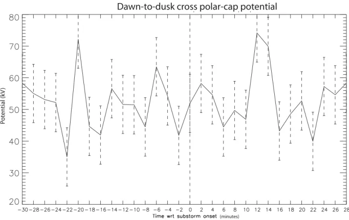
As in Sect. 4.4 the dawn-to-dusk flow reversal bound-ary is taken as a proxy for the polar cap boundbound-ary. For each time sample the anti-sunward component of the cosine-fitted velocity at each grid point is multiplied by the length of the dawn-to-dusk polar boundary along which it is ob-served. This is done all the way along the polar cap bound-ary and the individual potentials are then summed to create the cross polar-cap potential. Figure 12 presents the cross polar cap potential, from 30 min before substorm onset until 30 min after. The cross polar cap potential is not an abso-lute value, as no attempt has been made to compensate for the stretching/shrinking of the convection pattern performed when transforming the substorm convection patterns into the substorm co-ordinate system. However, as each substorm was stretched by the same amount over the entire time inter-val of the substorm, the inter-value of the cross polar cap potential presented represents the relative change of the cross cap potential during the substorm. The average cross polar-cap potential is 53±9 kV. The error bars presented on the graph is the standard deviation of the cross polar-cap poten-tial. Although there are rather large fluctuations in the dawn-to-dusk potential, some general trends can be observed. Dur-ing the substorm growth phase the dawn-to-dusk transpolar voltage is at a maximum of 72 kV 20 min before substorm onset. Just before substorm onset the transpolar voltage is

∼40 kV. The voltage reaches a maximum of 74 kV 12 min after onset.

4.6 Low-latitude velocity and potential

We determined the weighted mean of low-latitude return flow from the equatorward edge of the polar-cap boundary to the equatorward limit of the radar field-of-view across the dawn and dusk sectors, using the same method used to derive the mean high-latitude velocities described in Sect. 4.4. The mean was weighted by the number of points used to derive the cosine-fitted velocities. The velocities are presented in Fig. 13. Points that are different at a 95% confidence level are marked by an “x”. At almost all times the dusk velocity is significantly larger than the dawn velocity.

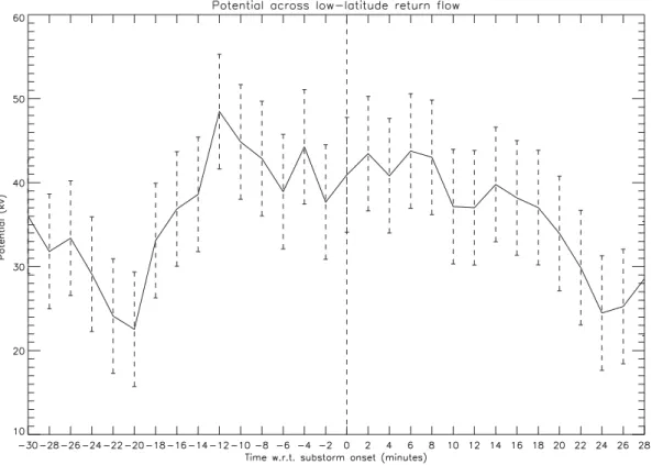
We calculated the low-latitude potential from the equa-torward edge of the polar cap boundary and to the edge of the convection pattern. This potential was calculated in the same way as we calculated the cross polar cap potential in Sect. 4.5. The results are presented in Fig. 14. The average low-latitude potential is 36±7 kV, with the standard deviation

presented as error bars in Fig. 14. The average low-latitude potential is much smaller than the average cross polar-cap potential. We would expect the two to be the same. We believe that this discrepancy is probably due to the edge of the convection pattern being equatorward of the equatorward edge of the SuperDARN field-of-view, causing the apparent saturation of the low-latitude potential at around 40–50 kV. There is a large difference in the low-latitude potentials served in the dawn and dusk sectors, with the potentials ob-served in the dusk sector considerably larger than the poten-tial observed in the dawn sector. This is due to the much larger velocities observed at low-latitude in the dusk sector as compared with the dawn sector. The velocities presented in Fig. 11 show that there is a general trend toward larger velocities in the dusk sector than in the dawn sector also at higher latitude, although this difference is much more pro-nounced at lower latitudes.

5 Discussion

In this study we have performed a statistical superposed epoch analysis of the flow during the growth and expansion phases of magnetospheric substorms, analysing the plasma flow from 30 min before substorm onset until 30 min after substorm onset for 67 substorms. No attempt has been made to identify the onset of the substorm recovery phase, although as the typical length of the substorm expansion phase is of the order of 30 to 60 min (Lui, 1991), we can assume that the majority of the substorms will not have progressed into the recovery phase during the intervals selected for this study.

Global grids of the cosine-fitted flow vectors are presented. During the substorm growth phase, strong flow was observed flowing into the polar cap on the dayside, and as the growth phase progressed, the strengths of these flow increased, such that they could be observed over a wider range of local times. As early as 20 min before substorm onset dayside plasma flows in the midday region were observed to become more structured and directed more towards the polar cap. During the growth phase the dawn-to-dusk transpolar voltage peaked 20 min before substorm onset, illustrating increased plasma flux flowing across the polar cap. The anti-sunward compo-nent of the plasma velocity flowing across the dawn sector of the polar cap peaked 18 min before onset. As the growth phase progressed, the equatorward and poleward boundaries of the nightside radar backscatter moved to lower latitudes.

The equatorward motion of HF backscatter during the sub-storm growth phase has been reported by Lewis et al. (1997), and has since been observed by a number of authors (e.g. Yeoman et al., 1999, 2000a; Provan et al., 2002; Milan et al., 2003). Such systematic equatorward motion of radar backscatter is believed to correspond to an equatorward mo-tion of the structured precipitamo-tion of the expanding auroral oval. This expansion is a result of unbalanced dayside recon-nection adding open flux to the polar cap during the growth phase, causing the poleward and equatorward edges of the polar cap to move to lower latitudes (McPherron, 1970).

(14)

(minutes)

Fig. 13. The anti-sunward component of the weighted mean flow velocity across the low-latitude return flow region (black line) and across

the dawn (blue line) and dusk (red line) sectors. The error bars are the standard error at each point.

(15)

3620 G. Provan et al.: Statistical study of high-latitude plasma flow Following substorm onset there is a reduction of

night-side radar backscatter. As the expansion phase evolves so too does this depletion in nightside backscatter. Many stud-ies have reported a lack of nightside HF radar data following expansion phase onset, due to the absorption of radio waves in the ionosphere (e.g. Lewis et al; 1997, Yeoman and L¨uhr, 1997; Lester, 2000) by the precipitating auroral electrons. Our statistical study demonstrates that this depletion in night-side backscatter occurs almost immediately following sub-storm onset, and that it further develops during the subsub-storm expansion phase, eventually affecting a sizeable part of the nightside ionosphere. Previous studies by, for example, Mi-lan et al., 1996 and MiMi-lan et al., 1999, have discussed the disruption of HF propagation during substorm onset.

During the expansion phase a region of suppressed flow is observed, initially covering a region from 22:30 to 24:00 MLT, and from ∼62◦ _{to ∼70}◦ _{MLT. Fast flows}

ap-pear to be deflected around this suppressed flow region, in such a manner that the basic two-cell convection pattern was preserved. Previous workers have also observed regions of nightside flow suppression when studying the ionospheric response to a substorm expansion phase, for example, Yeo-man et al. (2000a), Fox et al. (2001), Khan et al. (2001) and Grocott et al. (2002). It is likely that this suppressed flow region is related to the increased auroral and magnetic activity previously reported during the substorm expansion phase. For example, Khan et al., 2001, presented case studies of two complete “classic” substorm cycles where enhanced auroral brightening and increased magnetic activity was re-ported to be observed over a similar MLT/MLAT range and on a similar time scale as the suppressed flow region re-ported here. They also rere-ported that ionospheric flows within the substorm auroral bulge became semi-stagnant through-out the expansion phase. The surrounding flow generally remained vigorous and deflected around the semi-stagnant region. They believed such flow stagnation to be due to the high electrical conductivity of the bulge ionosphere com-pared with the surrounding region.

Opgenoorth and Pellinen (1998) observed an abrupt en-hancement in ionospheric flows in response to substorm on-set. They suggested that extreme dipolarisation of a magne-tospheric segment inside the substorm current wedge would result in a suppression of flow in this region, and the de-flection and relative enhancement of the flow around this re-gion. However, this deflection and resultant flow enhance-ment would not change the overall transpolar voltage. In Fig. 12 we present the dawn-to-dusk cross polar-cap poten-tial. The transpolar voltage is ∼40 kV just before substorm onset and increases to 74 kV 12 min after onset. This is despite the average IMF Bz component becoming

increas-ingly less negative from ∼5 min before substorm onset until

∼4 min after substorm onset. Such enhancement in the to-tal transpolar flux associated with substorm onset was pre-viously observed by Grocott et al. (2002) while studying an isolated substorms. The transpolar voltages derived by Gro-cott and co-workers (2002) are very similar to the voltage magnitudes presented here. Our detailed statistical study

clearly proves that nightside reconnection during substorm onset results in enhanced flux being driven across the polar cap.

In order to quantify the strength of the plasma flow across the polar-cap, and within the return flow, we presented the mean anti-sunward flow component across the polar-cap (Fig. 11) and across the low-latitude return flow region (Fig. 13). Figure 11 demonstrates that during the substorm growth phase the flow across the polar-cap is at a minimum 14 min before substorm onset, reaching a maximum 12 min after substorm. Figure 13 demonstrates that the magnitude of the return flow starts to increase at substorm onset and con-tinues until 8 min after substorm onset. Using the Student’s t-test we found that the variation in the return flow velocity observed at these two times was significant at the 95% confi-dence level. Flow excitation during larger substorms has also previously been reported by Sandholt et al. (2002).

It is thus clear that nightside reconnection occurring dur-ing the substorm expansion phase resulted in the excitation of new voltage and large-scale flow within the polar cap. This has previously been suggested by Lockwood et al. (1990) and Cowley and Lockwood (1992), although, to our knowledge, the results presented here are the first to prove this on a sta-tistical basis. We are not stating that the increase in plasma flow around the nightside suppressed flow region cannot also excite plasma flow, but the large increase in the transpolar voltage during the expansion phase onset would suggest that the main driver behind the excitation of large-scale plasma flow is nightside reconnection.

Studying the dawn-to-dusk transpolar voltage (Fig. 12) illustrates that between 6 min prior to substorm onset and 2 min prior to substorm onset the cross polar-cap potential decreases by approx. 20 kV. This would suggest that there is a decrease of plasma flow across the polar-cap immediately prior to substorm onset. The high-latitude plasma flows pre-sented in Fig. 11 also indicate a decrease in the plasma veloc-ity across the polar-cap between 2 min before substorm onset and 2 min after substorm onset. However, the large error bars associated with these velocities mean that this difference in velocity cannot be judged to be significant. A detailed anal-ysis of the transpolar voltage and high-latitude plasma flows associated with the few minutes immediately prior to and af-ter substorm onset will be an area of further research.

Figure 11 also presents the mean velocity across the dawn and dusk sectors of the polar cap. Although there are only 9 times during the substorm growth and expansion phases where there is a significant difference between the dawn and dusk velocities, at all these times the dusk velocities are sig-nificantly larger than the dawn velocities. Figure 13 shows that in the low-latitude return flow the dusk return flow is almost always larger than the dawn return flow. So there ap-pears to be a general trend that the dusk velocity is larger than the dawn velocity, especially at lower latitudes. We wondered whether this difference in the velocity between the dawn and dusk sectors could be due to the radars moving with the rotation of the Earth. In the return flow it would re-sult in faster velocities being observed in the dusk than dawn