Early Holocene Laurentide Ice Sheet deglaciation causes cooling in the high-latitude Southern Hemisphere through oceanic teleconnection

(1)

HAL Id: hal-02105658

https://hal.archives-ouvertes.fr/hal-02105658

Submitted on 21 Apr 2019

HAL is a multi-disciplinary open access

archive for the deposit and dissemination of

sci-entific research documents, whether they are

pub-lished or not. The documents may come from

teaching and research institutions in France or

abroad, or from public or private research centers.

L’archive ouverte pluridisciplinaire HAL, est

destinée au dépôt et à la diffusion de documents

scientifiques de niveau recherche, publiés ou non,

émanant des établissements d’enseignement et de

recherche français ou étrangers, des laboratoires

publics ou privés.

Early Holocene Laurentide Ice Sheet deglaciation causes

cooling in the high-latitude Southern Hemisphere

through oceanic teleconnection

H. Renssen, H. Goosse, X. Crosta, Didier M. Roche

To cite this version:

H. Renssen, H. Goosse, X. Crosta, Didier M. Roche. Early Holocene Laurentide Ice Sheet

deglacia-tion causes cooling in the high-latitude Southern Hemisphere through oceanic teleconnecdeglacia-tion.

Pa-leoceanography, American Geophysical Union, 2010, 25 (3), pp.PA3204. �10.1029/2009PA001854�.

�hal-02105658�

(2)

for

Full Article

Early Holocene Laurentide Ice Sheet deglaciation causes cooling

in the high

‐latitude Southern Hemisphere

through oceanic teleconnection

H. Renssen,

1

H. Goosse,

2

X. Crosta,

3

and D. M. Roche

1,4

Received 31 August 2009; revised 7 April 2010; accepted 7 May 2010; published 20 July 2010.

[1]

The impact of the early Holocene Laurentide Ice Sheet (LIS) deglaciation on the climate at Southern

Hemisphere high latitudes is studied in three transient simulations performed with a global climate model of the

coupled atmosphere

‐ocean‐vegetation system. Considering the LIS deglaciation, we quantify separately the

impacts of the background meltwater fluxes and the changes in topography and surface albedo. In our model,

the meltwater input into the North Atlantic results in a substantial weakening of the Atlantic meridional

overturning circulation, associated with absence of deep convection in the Labrador Sea. Northward ocean heat

transport by the Atlantic Ocean is reduced by 28%. This weakened ocean circulation leads to cooler North

Atlantic Deep Water (NADW). Upwelling of this cool NADW in the Southern Ocean results in reduced surface

temperatures (by 1°C to 2°C) here between 9 and 7 ka compared to an experiment without LIS deglaciation.

Poleward of the polar front zone, this advective teleconnection between the Southern and Northern hemispheres

overwhelms the effect of the

“classical” bipolar seesaw mechanism. These results provide an explanation for

the relatively cold climatic conditions between 9 and 7 ka reconstructed in several proxy records from Southern

Hemisphere high latitudes, such as Antarctic ice cores.

Citation: Renssen, H., H. Goosse, X. Crosta, and D. M. Roche (2010), Early Holocene Laurentide Ice Sheet deglaciation causes cooling in the high‐latitude Southern Hemisphere through oceanic teleconnection, Paleoceanography, 25, PA3204,

doi:10.1029/2009PA001854.

1. Introduction

[2] A central issue in climatology is to comprehend how the Northern and Southern hemispheres are coupled during periods of climate change [e.g., Jansen et al., 2007]. Many studies have suggested that past climate variability at Southern Hemisphere (SH) high latitudes has been linked to climate in the North Atlantic region through meltwater‐ induced perturbations of the Atlantic Meridional Overturning Circulation (AMOC) [e.g., EPICA Community Members, 2006]. Such an oceanic teleconnection appears especially evident for the last glacial, when warming in Antarctica coincided with cooling in the Northern Hemisphere during periods with massive iceberg discharges into the North Atlantic (i.e., Heinrich events), releasing substantial melt-water fluxes [e.g., Blunier and Brook, 2001; Ganopolski and Rahmstorf, 2001]. The “classical” explanation for this behavior of the climate system is the so‐called bipolar seesaw mechanism [Crowley, 1992; Broecker, 1998; Stocker, 1998].

[3] According to this bipolar seesaw concept, freshwater perturbations in the North Atlantic cause AMOC weakening and reduced northward heat transport by the Atlantic Ocean, resulting in relatively cool conditions in the North Atlantic region and relatively warm conditions in the South Atlantic Ocean due to the accumulation of heat [e.g., Barker et al., 2009]. The bipolar seesaw not only affects the Atlantic Ocean but also creates opposite temperature signals over practically the entire surface of both hemispheres. This is prominently seen in hosing experiments with coupled general circulation models in which a large amount of freshwater is injected at the surface of the North Atlantic Ocean, effectively causing a strong weakening of the AMOC [e.g., Stouffer et al., 2006].

[4] Compared to glacials, meltwater discharges during interglacials have been relatively small [Licciardi et al., 1999] and the impact on the global climate can be expected to have been modest. However, model studies suggest that the bipolar seesaw mechanism was in operation during the early Holocene 8.2 ka event, which has been associated with cat-astrophic drainage of proglacial Laurentide lakes and subse-quent disruption of the AMOC [e.g., Barber et al., 1999]. Simulations of the 8.2 ka event show cooling in the North Atlantic region, followed after a few decades of warming in the South Atlantic Ocean [Renssen et al., 2002; Wiersma and Renssen, 2006; LeGrande et al., 2006; Wiersma et al., 2008]. This model response has been corroborated by data from the South Atlantic region, showing evidence for a brief warm episode at the time of the North Atlantic cooling anomaly

1_{Section Climate Change and Landscape Dynamics, Department} of Earth Sciences, Faculty of Earth and Life Sciences, VU University Amsterdam, Amsterdam, Netherlands.

2

Institut d’Astronomie et de Ge´ophysique Georges Lemaıˆtre, Université Catholique de Louvain, Louvain‐la‐Neuve, Belgium.

3_{EPOC, UMR 5805, Université Bordeaux 1, CNRS, Talence, France.} 4

(3)

associated with the 8.2 ka event [Ljung et al., 2007; Ljung and Björck, 2008].

[5] In addition to the catastrophic lake drainage at 8.2 ka, the background melting of the Laurentide Ice Sheet (LIS) also had a freshening effect on the Atlantic Ocean, potentially weakening the AMOC [Bauer et al., 2004; Wiersma et al., 2006]. Indeed, marine proxy records suggest that deep water formation in the Labrador Sea only commenced after the LIS had disintegrated around 7 ka [Hillaire‐Marcel et al., 2001, 2007; de Vernal and Hillaire‐Marcel, 2006]. Although some modeling studies have considered the influence of the background LIS melting on the early Holocene climate in the Northern Hemisphere [Wang and Mysak, 2005; Wiersma et al., 2006; Renssen et al., 2009], the impact on the SH high latitudes has not yet been studied in detail. Therefore, the question remains to what extent early Holocene climate variability in the North Atlantic region and at SH high lati-tudes were coupled through oceanic teleconnections.

[6] To address this issue, we study here the impact of early Holocene LIS deglaciation on the climate of the SH high latitudes in a global coupled atmosphere‐ocean‐vegetation model. This paper is a follow‐up of an earlier study that analyzed the impact of orbital and greenhouse gas forcing on the climate evolution in Antarctica during the last 9000 years, using a transient simulation experiment performed with the same model [Renssen et al., 2005a]. The latter simula-tion could explain many characteristics of Holocene proxy records from the area, such as the long‐term cooling trend and a summer thermal optimum between 6 and 3 ka in eastern Antarctica. Renssen et al. [2005a] concluded that the long‐ term temperature trends could be explained by a combination of local orbital forcing and the long memory of the system, producing year‐round warm conditions in the Southern Ocean in the early Holocene. In the present study, we add the effect of LIS deglaciation. We concentrate on the millennial timescales and therefore do not consider forcings that are important at shorter timescales, such as solar and volcanic forcing and the effect of catastrophic lake drainage. The impact of these short‐term forcings was analyzed elsewhere [Renssen et al., 2001, 2002, 2006, 2007; Goosse and Renssen, 2004, 2006]. In a separate study [Renssen et al., 2009], we analyzed the impact of the early Holocene LIS deglaciation on the Northern Hemispheric climate.

2. Model and Experimental Design

[7] The model and experimental design have been described elaborately in a recent paper [Renssen et al., 2009],

so here only a summary is provided. We performed our simulations with ECBilt‐CLIO‐VECODE version 3, i.e., exactly the same global atmosphere‐ocean‐vegetation model as used by Renssen et al. [2005a]. The atmospheric module ECBilt is a quasi‐geostrophic model with T21L3 resolution [Opsteegh et al., 1998]. The oceanic component CLIO con-sists of a free‐surface, primitive‐equation oceanic general circulation model coupled to a dynamic‐thermodynamic sea ice model [Goosse and Fichefet, 1999]. CLIO has 20 levels in the vertical and a 3° × 3° latitude‐longitude horizontal reso-lution. VECODE is a vegetation model that simulates the dynamics of two main terrestrial plant functional types, trees and grasses, and desert as a dummy type [Brovkin et al., 2002]. ECBilt‐CLIO is capable of simulating a reasonable present‐day climate [Goosse et al., 2001; Renssen et al., 2002]. Further information about the model is available at http://www.knmi.nl/onderzk/CKO/ecbilt.html.

[8] We discuss three different transient experiments that cover the last 9000 years: ORBGHG, OGMELT, and OGMELTICE (Table 1). Our reference simulation, ORBGHG, is forced by long‐term orbital (Figure 1) and greenhouse gas forcing (Figure 2) and has been discussed in detail by Renssen et al. [2005a, 2005b]. It should be noted that we employed in our model a calendar with 360 days per year, with each month containing 30 days. The vernal equinox was fixed at day 81. This is common practice in Holocene climate modeling studies [e.g., Crucifix et al., 2002; Weber et al., 2004]. We realize that it would have been more appropriate to apply a calendar in which the duration of the months depends on their angular length [Joussaume and Braconnot, 1997], but as this would require substantial adjustments to our model, we chose to apply a calendar with months of equal duration for con-venience. This issue is especially relevant when considering seasonal model results.

[9] As explained by Renssen et al. [2009], we used for OGMELT the same setup as for ORBGHG, but additionally introduced freshwater to the Hudson Strait and St. Lawrence outlet, representing the background melting of LIS (Figure 3). The total additional freshwater flux between 9.0 and 8.4 ka was set to 0.09 Sv (1 Sv = 1 × 106m3/s), decreasing slightly to 0.08 Sv between 8.4 and 7.8 ka, finally dropping to 0.01 Sv between 7.8 and 6.8 ka. These freshwater rates are adjusted from estimates by Licciardi et al. [1999]. Compared to the latter study, we elevated the freshwater flux in the Hudson Strait between 9.0 and 8.4 ka by 0.04 Sv to ensure prevention of deepwater formation in the Labrador Sea, in accordance with Hillaire‐Marcel et al. [2001, 2007]. In OGMELTICE, we additionally included the impact of the disintegrating LIS during the period 9 to 7 ka by updating surface albedo and topography at 50 year time steps following Peltier [2004]. All other forcings (i.e., solar constant, aerosol content) were kept constant at preindustrial values. To obtain initial con-ditions for OGMELT and OGMELTICE, we ran the model for 1000 years with appropriate forcings for 9 ka (meltwater flux in OGMELT, meltwater flux plus LIS albedo and topography in OGMELTICE), starting from a state derived from ORBGHG.

[10] The differences between the three experiments enable us to analyze the impact of the LIS. The difference between OGMELT and ORBGHG provides information on the effect

Table 1. Summary of Experimentsa

Experiment Name Forcings

ORBGHG Orbital and greenhouse (CO2and CH4)

OGMELT Orbital, greenhouse, and LIS background meltflux OGMELTICE Orbital, greenhouse, LIS background meltflux, and

LIS surface albedo and topography

a_{The ORBGHG experiment represents the response to orbital (Figure 1)} and greenhouse gas (Figure 2) forcing. OGMELT includes an additional freshwater forcing (Figure 3), describing the LIS background LIS meltflux. OGMELTICE additionally includes the LIS topography and surface albedo and thus describes the total response to all considered forcings.

RENSSEN ET AL.: EARLY HOLOCENE COOLING IN SOUTHERN OCEAN PA3204 PA3204

(4)

Figure 2. Applied greenhouse gas forcing: atmospheric concentrations of CO2and CH4based on ice core

measurements [Raynaud et al., 2000].

Figure 1. Applied orbital forcing [Berger, 1978]. (top) Insolation at 60°N and (bottom) 60°S, shown as the anomaly relative to 0 ka. In our simulations, insolation varies annually per latitude.

(5)

of the background meltflux of the LIS, while the difference between OGMELTICE and OGMELT represents the com-bined impact of the LIS surface albedo and topography. Finally, the OGMELTICE minus ORBGHG anomaly gives information on the total influence of the LIS on climate.

[11] It should be noted that we neglect in our experiments the impact of Holocene deglaciation in Antarctica. Recent experiments focused on future Antarctic ice sheet melting suggest a negative feedback on anthropogenic warming through the formation of a cold halocline in the Southern Ocean that limits sea ice retreat, leading to a relatively enhanced surface albedo [Swingedouw et al., 2008]. More-over, in these experiments the formation of Antarctic Bottom Water (AABW) is reduced, which moderates the weakening

of AMOC under global warming scenarios. Although the amount of Antarctic melting during the early Holocene is uncertain, it is possible that similar effects as noted for future warming were important at that time. This should be kept in mind when interpreting our results.

3. Results and Discussion

3.1. Global Surface Temperature Response

[12] A comparison of the global sea surface temperature (SST) response in the three experiments clearly shows the cooling effect of the remnant LIS in the early Holocene (Figure 4). From 9 to 8 ka, the annual mean SSTs are 0.15°C lower in OGMELT than in ORBGHG and even more than Figure 3. Applied background freshwater forcing (in Sv = 106m3s−1), representing the LIS

background melt rate, introduced in the St. Lawrence outlet and Hudson Strait in experiments OGMELT and OGMELTICE. This forcing is adjusted from Licciardi et al. [1999].

Figure 4. Simulated annual global SST anomaly (°C) relative to the preindustrial mean. Shown are the results for ORBGHG (black), OGMELT (dark gray), and OGMELTICE (light gray). A 499 year running mean was applied.

(6)

0.3°C lower in OGMELTICE. Assuming a linear rela-tionship, the LIS background melting and the LIS ice thus contribute more or less equally to the cool early Holocene conditions on a global scale. After 8 ka, temperatures in OGMELT and OGMELTICE rapidly increase, and when the LIS is gone at 6 ka, the SSTs are at the same level as in ORBGHG.

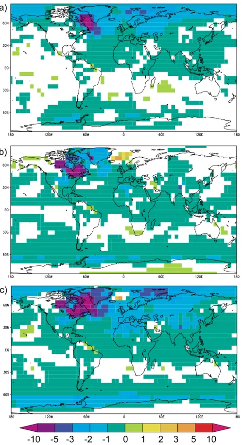
[13] As discussed in detail by Renssen et al. [2009], these cooler conditions in OGMELT and OGMELTICE compared to ORBGHG are particularly evident in the Northern Hemi-sphere middle and high latitudes. Comparing OGMELT with ORBGHG (Figure 5) shows that the LIS background melting reduced temperatures over the Labrador Sea (more than 10°C cooler) close to where the freshwater enters the ocean. Over the Arctic Ocean, Greenland and northern Eurasia, conditions are also clearly cooler in OGMELT, with a maximum dif-ference of more than 3°C over the Barents Sea area. The cooling influence of the LIS ice is most clearly seen over the ice sheet itself (more than 10°C) and downwind areas, par-ticularly Greenland and the North Atlantic Ocean surface (Figures 5a, 5c, and 6b). The LIS ice also causes modest warming over a small area east of Iceland.

[14] Over the Southern Ocean the LIS impact also produces cooler conditions compared to ORBGHG. In the latter experiment, the Southern Ocean surface, particularly over the Pacific and Atlantic sectors south of 60°S, is at 9 ka up to 2°C warmer on an annual basis than at 0 ka. In OGMELT, these relatively warm early Holocene conditions are less evident, and in OGMELTICE the Southern Ocean is generally slightly cooler at 9 ka than at 0 ka. Consequently, both the LIS background meltflux and the LIS ice cool the Southern Ocean (Figure 6). The total cooling effect of the LIS amounts to 1°C to 2°C (Figure 6c). At lower latitudes, the effect of LIS deglaciation is minor. Over the South Atlantic Ocean between 10°S and 40°S a small increase in temperature is noted, but this is mostly outside the 95% significance level (Figure 6c). How can we explain these temperature patterns? The main answer must be sought in the oceanic response to LIS deglaciation, particularly in the Atlantic Basin.

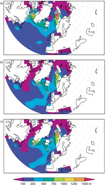
3.2. Response of the Atlantic Ocean Circulation [15] The surface ocean freshening associated with the LIS background meltflux prevents the formation of deep water in the Labrador Sea that is evident in ORBGHG (Figures 7a and 7b). This absence of deep convection in the Labrador Sea in the early Holocene is consistent with paleoceano-graphical evidence, indicating that deep water formation in the Labrador Sea only commenced after the LIS had com-pletely disintegrated at∼7 ka [Hillaire‐Marcel et al., 2001, 2007]. In the Nordic seas, the convection depth is also reduced in OGMELT compared to ORBGHG, but here deepwater is still formed south of Svalbard (i.e., mixed layer depth reaches 1000 m). The cooling effect of the LIS ice in OGMELTICE partly counteracts the impact of freshening and enhances the convective activity (Figure 7c) relative to OGMELT, evidenced by deeper convection in the Nordic seas (more than 1500 m) and south of Greenland (reaching 1000 m). This is mainly due to the additional cooling of the North Atlantic Ocean surface, resulting in increased density of the surface layer compared to OGMELT.

[16] The meridional overturning stream function indicates a weakened North Atlantic Deep Water (NADW) cell in OGMELT compared to ORBGHG (Figure 8), consistent with the noted anomalies in convective activity due to the surface freshening. The maximum of the overturning strength is reduced by about 9 Sv (1 Sv = 1 × 106 m3 s−1), and the export of NADW at 30°S is reduced by about 3 Sv (Figures 8a, 8b, 8d, and 9a). In OGMELTICE, the NADW cell is slightly stronger than in OGMELT, with the maximum overturning strength being enhanced by 1 Sv due to the sole influence of the LIS ice (Figures 8c and 8e). After most of the background melting has stopped at 7.8 ka, the AMOC quickly strengthens in OGMELT up to the level of ORBGHG (i.e., NADW export at 30°S of 13.5 Sv, Figure 9a), showing that the effect of surface ocean freshening on the ocean circulation becomes less important. However, this is not the case in the experiment with the combined effect of LIS meltwater and ice, where the AMOC remains in a relatively weak inter-mediate state until 6.5 ka (NADW export of about 12 Sv), associated with the absence of deep convection in the Lab-rador Sea. Thus, including the LIS ice delays the AMOC recovery compared to OGMELT. The cooling effect of the LIS ice in OGMELTICE causes the Labrador Sea to remain ice covered in winter between 7.8 and 6.5 ka, preventing deep convection here until the LIS is gone.

[17] This timing agrees reasonably well with paleoceano-graphic data, suggesting initiation of Labrador Sea deep convection and decreasing sea ice cover in the western part of the Labrador Sea around 7 ka [Hillaire‐Marcel et al., 2007]. This is also consistent with several reconstructions suggesting that modern Atlantic Ocean circulation was established by 7–8 ka [Marchitto et al., 1998; Oppo et al., 2003; Piotrowski et al., 2004; Thornalley et al., 2010]. Other studies, however, indicate a slightly earlier timing of ∼8.5 ka [McManus et al., 2004; Roberts et al., 2010].

[18] The evolution of the northward heat transport by the Atlantic Ocean is clearly very similar to that of the Atlantic Ocean circulation strength (Figure 9b), showing that the LIS has an impact on the heat exchange between the Southern and Northern hemispheres through the deep ocean. From 9 to 8 ka, the northward heat transport is 0.09 PW less (i.e., reduced by 28%) in the experiments with the LIS influence compared to ORBGHG. After 6.5 ka, the AMOC is at a stable level, indicating that the changes in orbital and greenhouse gas forcing have no dominant influence on the trend in AMOC strength.

3.3. Response of Deep North Atlantic Temperature and the Link With Southern Ocean Surface Conditions

[19] It is clear that the cooling of the Southern Ocean’s surface discussed in section 3.1. is not consistent with the classical bipolar seesaw response. Analysis of a latitude‐ depth cross section of Atlantic Ocean temperatures (Figure 10) reveals that the cooler Southern Ocean is related to the 0.5°C to 1°C colder deep ocean at the depth of the main NADW export (between about 1500 and 3500 m) in the early Holo-cene in the experiments with the LIS influence (Figure 10). A comparison of the different experiments reveals that both the effects of LIS meltwater and LIS ice contribute to this deep ocean cooling. This can be expected, since both effects create

(7)

Figure 5. (a–c) Simulated 9 ka minus 0 ka annual mean temperatures (in °C) for the experiments ORBGHG, OGMELT, and OGMELTICE. Only results that are statistically significant at a 95% level (rel-ative to the 0 ka climate) are shown. Areas with statistically insignificant results are in white.

(8)

Figure 6. Simulated 9 ka annual temperature anomalies (in °C). (a) OGMELT minus ORBGHG (effect LIS melt), (b) OGMELTICE minus OGMELT (effect LIS ice), and (c) OGMELTICE minus ORBGHG (total effect LIS). Only results that are statistically significant at a 95% level (relative to ORBGHG 9 ka result) are shown. Areas with statistically insignificant results are in white.

(9)

a cooler North Atlantic Ocean surface (Figures 5 and 6), i.e., the source region of NADW. The deep North Atlantic is also cooler because of the change in deep convection patterns noted in Figure 7. In ORBGHG, two distinct water masses contribute to NADW, with different source regions, namely, Labrador Sea Water and the waters that form in the Nordic seas. In the experiments with the LIS impact, however, the Labrador Sea deep convection is shut down in the early Holocene, while deep water is still formed in the Nordic seas. Since the source waters in the Nordic seas are cooler than in the Labrador Sea, this leads to relative cooling of NADW.

[20] The Southern Ocean is characterized by a large‐scale upwelling in the model as observed in the real ocean [Jacques and Tréguer, 1986]. Consequently, the negative oceanic temperature anomaly at depth is transferred upward between

70°S and 40°S. When the colder water reaches the surface, the temperature anomaly is amplified by classical feedbacks, implying sea ice leading to a surface cooling that reaches more than 2°C in some regions. Such a transport of temper-ature anomaly from the North Atlantic to the Southern Ocean has been postulated by Crowley and Parkinson [1988] and has also been observed and previously analyzed in idealized experiments and in simulations covering the past millennium with the same model [Goosse et al., 2004]. In the latter study, the lag between the North Atlantic surface cooling and the upwelling of cold waters in the Southern Ocean was on the order of 100–200 years.

[21] Consequently, the cooler early Holocene conditions in the Southern Ocean due to the LIS are clearly reflected by much more sea ice compared to the simulation with only orbital and greenhouse gas forcing (Figure 11). The sea ice volume is substantially higher (by about 1 × 103km3) at 9 ka in OGMELTICE than at 0 ka. This relatively extensive sea ice cover is present in both winter and summer (not shown) and results in much lower annual mean surface air temperatures over the Southern Ocean south of 60°S seen in Figure 6c. Especially in the Atlantic sector, the expanded sea ice cover reduces slightly the formation of AABW, explaining why the AABW cell in the Atlantic Ocean is not enhanced in OGMELTICE compared to ORBGHG (Figure 8f). After 7 ka, the effect of the LIS on the SH sea ice is no longer visible. Comparison of OGMELT and OGMELTICE firms that both the LIS melt and LIS ice effects have con-tributed to the cold early Holocene conditions in the Southern Ocean. As a result of the LIS influence, the timing of the onset of the warmest conditions of the last 9000 years is thus delayed from 9 to 7 ka compared to ORBGHG. In our OGMELTICE simulation, temperatures in all seasons show this delaying effect (not shown), although it should be noted that the timing of peak warming differs between summer (around 4 ka) and spring (around 7 ka), as has been discussed similarly by Renssen et al. [2005a] for ORBGHG.

[22] At the scale of the Atlantic Ocean, the seesaw response is overwhelmed by the effect of the upwelling of cooler NADW. Along with the cooler surface conditions in the Southern Ocean due to the discussed teleconnection between the North Atlantic and the Southern oceans, including the LIS influence also results in slight warming (up to 1°C) at shallow depths between 50 and 400 m (Figure 10), mostly at SH midlatitudes. This shows that some heat accumulation occurs in the South Atlantic as a result of the less effective northward heat transport by the AMOC (bipolar seesaw), but this has no strong effect at the surface ocean, although a small (but mostly statistically insignificant) increase in SSTs is found between 30°S and 40°S (Figure 6).

[23] Over the Southern Ocean, the simulated 9 ka heat flux at the atmosphere‐ocean interface is consistent with the dis-cussed upwelling of cold water that generally overwhelms the seesaw effect (Figure 12a). Centered at 60°S there is a clear increase in the heat flux of up to 15 W m−2(indicating heat loss for the atmosphere) that is related to the relatively cold ocean surface in OGMELTICE. Here the maximum expan-sion in sea ice cover also occurs, with annual mean sea ice concentration fraction being up to 0.15 higher (Figure 12b). Figure 7. Simulated 9 ka February mixed layer depth (m)

for (a) ORBGHG, (b) OGMELT, and (c) OGMELTICE.

(10)

Over the expanded sea ice strong cooling of the atmosphere takes place, and north of the sea ice edge the atmosphere is still cooler than the ocean, reflected by decreased heat flux, indicating heat loss for the ocean (up 10 W m−2). This

is particularly evident in the zone north of the Antarctic Peninsula. Farther north, there is also a zone with ocean heat loss (more than 5 W m−2), particularly in the South Atlantic between 30°S and 40°S. This is the area where SSTs are Figure 8. Simulated meridional overturning streamfunction at 9 ka in the Atlantic Ocean Basin.

(a) ORBGHG, (b) OGMELT, (c) OGMELTICE, (d) OGMELT minus ORBGHG (effect LIS melt), (e) OGMELTICE minus OGMELT (effect LIS ice), and (f) OGMELTICE minus ORBGHG (total effect LIS). Positive values denote clockwise flow in Sv.

(11)

slightly higher in OGMELTICE than in ORBGHG in response to the weakening of the northward heat transport by the AMOC (i.e., bipolar seesaw).

[24] In summary, in our model there is an oceanic tele-connection between the North Atlantic and the Southern Ocean that creates surface temperature anomalies of the same sign during the early Holocene. To make a clear distinction from the bipolar seesaw mechanism, we call this the advec-tive connection.

3.4. Evaluation Using Proxy Evidence

[25] Our simulations clearly suggest that the early Holo-cene LIS deglaciation had a cooling influence on the SH high latitudes until∼7 ka. Can we find confirmation in proxy

re-cords for this result? There is no simple answer to this question, as proxy records at SH high latitudes do not provide one consistent picture of centennial‐ to millennial‐scale cli-mate variability during the Holocene. This can be partly related to the strong spatial heterogeneity of SH high latitude climate. For instance, observations of recent variations in sea ice area show opposing trends in different Southern Ocean sectors [e.g., Stammerjohn and Smith, 1997; Stammerjohn et al., 2008; Lefebvre and Goosse, 2008]. On the other hand, different proxies may have registered different seasons, resulting in different timings of thermal optima [cf. Renssen et al., 2005a]. There is also no SST record south of 60°S, where the maximum cooling is observed. Quantitative reconstructions are generally from the Polar Front Zone Figure 9. (a) Simulated export of NADW and (b) northward heat transport by the Atlantic Ocean at 20°S.

Shown are the results of ORBGHG (black), OGMELT (dark gray), and OGMELTICE (light gray) as 499 year running means.

(12)

Figure 10. Simulated north‐south temperature‐depth profile (in °C) in the Atlantic basin at 9 ka averaged over 65°W to 10°E. Shown are (a) OGMELT minus ORBGHG (effect LIS melt), (b) OGMELTICE minus OGMELT (effect LIS ice), and (c) OGMELTICE minus ORBGHG (total effect LIS).

(13)

around 54°S to 50°S, where the simulated cooling is very small. In addition, some records have a low temporal reso-lution that does not permit a detailed analysis of the climatic conditions in the early Holocene, and furthermore, the mod-eled cooling is often within the error bars of the reconstructed temperature anomalies.

[26] Some records suggest a cool phase during the early Holocene, more or less in agreement with our results. For instance, Antarctic ice cores show a relatively cool period between an early Holocene thermal optimum from 11.5 to 9 ka, and a secondary optimum that varied in timing between 7– 5 ka (Ross Sea sector) and 6–3 ka (Eastern Antarctica) [Masson et al., 2000; Jouzel et al., 2001; Masson‐Delmotte et al., 2004]. This is consistent with marine diatom records from the Atlantic sector south of the polar front, suggesting a thermal optimum between 12 and 9 ka, followed by cooling and sea ice expansion between 9 and 7 ka [Bianchi and Gersonde, 2004]. Diatom records from the Antarctic Penin-sula provide evidence for the second thermal optimum between 8–7 and 4–3 ka [Taylor et al., 2001; Heroy et al., 2008]. East Antarctic coastal diatom records also reveal a cool phase between 9 and 7.5 ka with extended sea ice cover, followed by a climatic optimum lasting until about 4 ka [Crosta et al., 2007, 2008; Denis et al., 2009]. The cooling between 9 and 7 ka seems more prominent at high southern latitudes, in agreement with the modeled LIS impact.

[27] Other records suggest a different climate evolution. For instance, some diatom records and terrigenous proxies from the Antarctic Peninsula suggest that the 9 to 7 ka period was relatively warm [e.g., Sjunneskog and Taylor, 2002; Brachfeld et al., 2002; Roberts et al., 2008]. Some diatom records from the Atlantic sector suggest generally warm conditions in the earliest Holocene, followed by a cooling trend that is from time to time briefly interrupted by cooler episodes [Hodell et al., 2001; Nielsen et al., 2004; Anderson et al., 2009]. Several records from eastern Antarctica show a variety of responses [e.g., Wagner and Melles, 2007].

[28] Following our results, we can hypothesize that the influence of the LIS deglaciation through the cold NADW teleconnection was responsible for the relatively cold phase recorded between 9 and 7–6 ka in Antarctic ice cores and other records. The subsequent thermal optimum between 7–6 and 4–3 ka could then represent the main impact of orbital forcing as discussed by Renssen et al. [2005a]. In addition, we may also speculate that the first thermal optimum (11.5 to 9 ka in ice cores) reflects conditions when AMOC was more severely weakened than between 9 and 7 ka, leading to a dominance of the classical bipolar seesaw teleconnection and relatively warm conditions at SH high latitudes. Such con-ditions were obtained by Wiersma et al. [2006] using the same model when they perturbed an early Holocene equi-librium climate state without Labrador Sea deep convection (resembling our early Holocene state in OGMELTICE) by introducing freshwater pulses resembling the evidence for catastrophic lake drainage just associated with the 8.2 ka event. Because of these freshwater pulses, the maximum overturning in the Atlantic Ocean was reduced by an addi-tional 25%, and a seesaw response resulted in a warming of 0.5°C to 1°C in the Southern Ocean [Wiersma et al., 2008]. If this explanation for the first Holocene thermal optimum is true, it implies that there was a strong oceanic teleconnection active between both hemispheres during the early Holocene. It can then be expected that similar hemispheric connections existed during earlier deglaciations.

[29] It should be noted that the sensitivity to freshwater perturbations is highly model dependent. For instance, a recent model intercomparison study in which different models (including ECBilt‐CLIO) were perturbed with the same freshwater perturbations in the North Atlantic Ocean revealed large variations in the magnitude of the simulated AMOC weakening and in the associated climate responses [Stouffer et al., 2006]. In the latter study, however, none of the models simulated a surface cooling in the Southern Ocean in response to a North Atlantic freshwater perturbation, Figure 11. Simulated Southern Hemisphere annual mean sea ice volume. Shown are the results for

ORBGHG (black), OGMELT (dark gray), and OGMELTICE (light gray). A 499 year running mean is applied.

(14)

although a few other model studies have shown this response [e.g., Manabe and Stouffer, 1997; Lohmann, 2003]. In our model, an essential requirement for the advective connection

to dominate over the bipolar seesaw mechanism is that the Labrador Sea deep convection is shut down because of a local meltwater influx, while the Nordic seas deep convection remains active, leading to a substantial cooling of the NADW that subsequently upwells in the Southern Ocean. The bipolar seesaw mechanism would dominate if also the Nordic seas deep convection is shut down; for instance, due to a larger meltwater perturbation or a freshwater release at a location close to the Nordic seas. In other words, our study suggests that the response of the climate at SH high latitudes to North Atlantic freshwater perturbations depends on the type of freshwater forcing (location and amount). In addition, the characteristics of the mean climate state that is perturbed (e.g., with or without LIS) affect this response.

4. Conclusions

[30] We have applied a coupled atmosphere‐ocean‐ vegetation model to study the impact of early Holocene LIS deglaciation on the climate of SH high latitudes. Our results suggest the following.

[31] 1. The LIS deglaciation resulted in a relatively cold Early Holocene climate at Southern Hemisphere high lati-tudes between 9 and 7 ka, with both LIS meltwater and LIS ice contributing to this cooling. Compared to a simulation without the LIS influence, annual mean surface temperatures were 1°C to 2°C lower over the Southern Ocean.

[32] 2. The cooler conditions are mainly related to upwelling of relatively cool waters in the Southern Ocean. Both the LIS meltwater and LIS ice cool the surface of the North Atlantic Ocean, leading to cooling of the source waters for NADW, thus also resulting in cooling of the deep North Atlantic Ocean between 1500 and 3500 m water depth. Part of this relatively cool water upwells in Southern Ocean, contributing to cooler climate in the early Holocene, signi-fying an advective connection.

[33] 3. The AMOC was weaker compared to the period after LIS deglaciation (i.e., after 7 to 6 ka), with the northward heat transport by the Atlantic Ocean reduced by 28%. This is particularly due to the absence of deep convection in the Labrador Sea in association with the meltwater flux from the LIS. Some accumulation of heat in the South Atlantic was associated with this weakened AMOC, in agreement with the bipolar seesaw principle, but this effect was overwhelmed in the Southern Ocean by the upwelling of relatively cold waters.

[34] 4. These results provide a plausible explanation for the relatively cold conditions between 9 and 7 ka reconstructed in several proxy records from SH high latitudes.

[35] Acknowledgments. H.G. is a research associate with the Fonds National de la Recherche Scientifique (Belgium) and is supported by the Bel-gian Federal Science Policy Office. D.M.R is supported by the Netherlands Organization for Scientific Research (NWO) in the framework of the RAPID project ORMEN and by INSU/CNRS.

References

Anderson, R. F., S. Ali, L. I. Bradtmiller, S. H. H. Nielsen, M. Q. Fleisher, B. E. Anderson, and L. H. Burckle (2009), Wind‐driven upwelling

in the Southern Ocean and the deglacial rise in atmospheric CO2, Science, 323, 1443–1448. Barber, D. C., et al. (1999), Forcing of the cold event of 8,200 years ago by catastrophic

drainage of Laurentide lakes, Nature, 400, 344–348.

Barker, S., P. Diz, M. J. Vautraves, J. Pike, G. Knorr, I. R . Hall, and W. S. Broecker

Figure 12. Simulated annual mean OGMELTICE minus ORBGHG anomalies (total effect LIS) at 9 ka for (a) atmosphere‐to‐ocean heat flux (in W m−2_{), with negative}

fluxes signifying ocean heat loss, and (b) sea ice concentra-tion (fracconcentra-tion).

(15)

(2009), Interhemispheric Atlantic seesaw response during the last deglaciation, Nature, 457, 1097–1102.

Bauer, E., A. Ganopolski, and M. Montoya (2004), Simulation of the cold climate event 8200 years ago by meltwater outburst from L a k e A g a s s i z , P a l e o c e an o g r a p hy , 1 9 , PA3014, doi:10.1029/2004PA001030. Berger, A. L. (1978), Long‐term variations of

daily insolation and Quaternary climatic changes, J. Atmos. Sci., 35, 2363–2367. Bianchi, P., and R. Gersonde (2004), Climate

evolution at the last deglaciation: The role of the Southern Ocean, Earth Planet. Sci. Lett., 228, 407–424.

Blunier, T., and E. J. Brook (2001), Timing of millennial‐scale climate change in Antarctica and Greenland during the last glacial period, Science, 291, 109–112.

Brachfeld, S. A., S. K. Banerjee, Y. Guyodo, and G. D. Acton (2002), A 13,200 year history of century to millennial‐scale paleoenvironmen-tal change magnetically recorded in the Palmer Deep, western Antarctic Peninsula, Earth Planet. Sci. Lett., 194, 311–326.

Broecker, W. S. (1998), Paleocean circulation during the last deglaciation: A bipolar seesaw?, Paleoceanography, 13, 119–121.

Brovkin, V., J. Bendtsen, M. Claussen, A. Ganopolski, C. Kubatzki, V. Petoukhov, and A. Andreev (2002), Carbon cycle, vegeta-tion, and climate dynamics in the Holocene: Experiments with the CLIMBER‐2 model, Global Biogeochem. Cycles, 16(4), 1139, doi:10.1029/2001GB001662.

Crosta, X., M. Debret, D. Denis, M. A. Courty, and O. Ther (2007), Holocene long‐ and short‐term climate changes off Adelie Land, East Antarctica, Geochem. Geophys. Geosyst., 8, Q11009, doi:10.1029/2007GC001718. Crosta, X., D. Denis, and O. Ther (2008), Sea ice

seasonality during the Holocene, Adélie Land, East Antarctica, Mar. Micropaleontol., 66, 222–232.

C r o w l e y , T . J . ( 1 9 9 2 ) , N o r t h A t l a n t i c Deep Water cools the Southern Hemisphere, Paleoceanography, 7, 489–497.

Crowley, T. J., and C. L. Parkinson (1988), Late Pleistocene variations in Antarctic sea ice II: Effect of interhemispheric deep‐ocean heat exchange, Clim. Dyn., 3, 93–103.

Crucifix, M., M. F. Loutre, P. Tulkens, T. Fichefet, and A. Berger (2002), Climate evolution during the Holocene: A study with an Earth system model of intermediate complexity, Clim. Dyn., 19, 43–60.

Denis, D., et al. (2009), Glacier and deep water Holocene dynamics, Adélie Land region, East Antarctica, Quat. Sci. Rev., 28, 1291–1302, doi:10.1016/j.quascirev.2008.12.024. de Vernal, A., and C. Hillaire‐Marcel (2006),

Provincialism in trends and high frequency changes in the northwest North Atlantic during the Holocene, Global Planet. Change, 54, 263–290.

EPICA Community Members (2006), One‐to‐ one coupling of glacial climate variability in Greenland and Antarctica, Nature, 444, 195–198.

Ganopolski, A., and S. Rahmstorf (2001), Rapid changes of glacial climate simulated in a coupled climate model, Nature, 409, 153–158. Goosse, H., and T. Fichefet (1999), Importance of ice‐ocean interactions for the global ocean circulation: A model study, J. Geophys. Res., 104, 23,337–23,355.

Goosse, H., and H. Renssen (2004), Exciting natural modes of variability by solar and volcanic forcing: Idealized and realistic experi-ments, Clim. Dyn., 23, 153–163.

Goosse, H., and H. Renssen (2006), Regional response of the climate system to solar forcing: The role of the ocean, Space Sci. Rev., 125, 227–235.

Goosse, H., F. M. Selten, R. J. Haarsma, and J. D. Opsteegh (2001), Decadal variability in high northern latitudes as simulated by an intermediate‐complexity climate model, Ann. Glaciol., 33, 525–532.

Goosse, H., V. Masson‐Delmotte, H. Renssen, M. Delmotte, T. Fichefet, V. Morgan, T. van Ommen, B. K. Khim, and B. Stenni (2004), A late medieval warm period in the Southern Ocean as a delayed response to external forc-ing?, Geophys. Res. Lett., 31, L06203, doi:10.1029/2003GL019140.

Heroy, D. C., C. Sjunneskog, and J. B. Anderson (2008) Holocene climate change in the Brans-field Basin, Antarctic Peninsula: Evidence from sediment and diatom analysis, Antarct. Sci., 20, 69–87.

Hillaire‐Marcel, C., A. de Vernal, G. Bilodeau, and A. J. Weaver (2001), Absence of deep‐ water formation in the Labrador Sea during the last interglacial period, Nature, 410, 1073–1077.

Hillaire‐Marcel, C., A. de Vernal, and D. J. W. Piper (2007), Lake Agassiz final drainage event in the northwes t North A tlantic, Geophys. Res. Lett., 34, L15601, doi:10.1029/ 2007GL030396.

Hodell, D. A., S. L. Kanfoush, A. Shemesh, X. Crosta, C. D. Charles, and T. P. Guilderson (2001), Abrupt cooling of Antarctic sur-face waters and sea ice expansion in the South Atlantic sector of the Southern Ocean at 5000 cal yr BP, Quat. Res., 56, 191–198. Jacques, J., and P. Tréguer (1986), Ecosystèmes

Marins Pélagiques, Collect. Écol., vol. 19, 243 pp., Masson, Paris.

Jansen, E., et al. (2007), Palaeoclimate, in Climate Change 2007: The Physical Science Basis: Con-tribution of Working Group I to the Fourth Assessment Report of the Intergovernmental Panel on Climate Change, edited by S. Solomon et al., pp. 433–498, Cambridge Univ. Press, New York.

Joussaume, S., and P. Braconnot (1997), Sensitivity of paleoclimate simulation results to season definitions, J. Geophys. Res., 102, 1943–1956.

Jouzel, J., et al. (2001), A new 27 ky high reso-lution East Antarctic climate record, Geophys. Res. Lett., 28, 3199–3202.

Lefebvre, W., and H. Goosse (2008), An anal-ysis of the atmospheric processes driving the large‐scale winter sea‐ice variability in the Southern Ocean. J. Geophys. Res., 113, C02004, doi:10.1029/2006JC004032. LeGrande, A. N., G. A. Schmidt, D. T. Shindell,

C. V. Field, R. L. Miller, D. M. Koch, G. Faluvegi, and G. Hoffmann (2006), Consis-tent simulations of multiple proxy responses to an abrupt climate change event, Proc. Natl. Acad. Sci. U. S. A., 103, 837–842.

Licciardi, J. M., J. T. Teller, and P. U. Clark (1999), Freshwater routing by the Laurentide ice sheet during the last deglaciation, in Mechanisms of Global Climate Change at Millennial Time Scale, Geophys. Monogr. Ser., vol. 112, edited by P. U. Clark et al., pp. 177–201, AGU, Washington, D. C.

Ljung, K., and S. Björck (2007), Holocene cli-mate and vegetation dynamics on Nightingale Island, South Atlantic—an apparent intergla-cial bipolar seesaw in action?, Quat. Sci. Rev., 26, 3150–3166.

Ljung, K., S. Björck, H. Renssen, and D. Hammarlund (2008), South Atlantic island record reveals South Atlantic response to 8.2 kyr BP event, Clim. Past, 4, 35–45. Lohmann, G. (2003), Atmospheric and oceanic

freshwater transport during weak Atlantic overturning circulation, Tellus, Ser. A, 55, 438–449.

Manabe, S., and R. J. Stouffer (1997), Coupled ocean‐atmosphere model response to fresh-water input: Comparison to Younger Dryas event, Paleoceanography, 12, 321–336. Marchitto, T. M., W. B. Curry, and D. W. Oppo

(1998), Millennial‐scale changes in North Atlantic circulation since the last glaciation, Nature, 393, 557–561.

Masson, V., et al. (2000), Holocene climate variability in Antarctica based on 11 ice‐core isotopic records, Quat. Res., 54, 348–358. Masson‐Delmotte, V., B. Stenni, and J. Jouzel

(2004), Common millennial‐scale variability of Antarctic and Southern Ocean temperatures during the past 5000 years reconstructed from the EPICA Dome C ice core, Holocene, 14, 145–151.

McManus, J. F., R. Francois, J.‐M. Gherardi, L. D. Keigwin, and S. Brown‐Leger (2004), Collapse and rapid resumption of Atlantic meridional circulation linked to deglacial cli-mate changes, Nature, 428, 834–837. Nielsen, S. H. H., N. Koc, and X. Crosta (2004),

Holocene climate in the Atlantic sector of the Southern Ocean: Controlled by insolation or oceanic circulation?, Geology, 32, 317–320. Oppo, D. W., J. F. McManus, and J. L. Cullen

(2003), Deepwater variability in the Holocene epoch, Nature, 422, 277–278.

Opsteegh, J. D., R. J. Haarsma, F. M. Selten, and A. Kattenberg (1998), ECBILT: A dynamic alternative to mixed boundary conditions in ocean models, Tellus, Ser. A, 50, 348–367. Peltier, W. (2004), Global glacial isostasy and

the surface of the ice‐age Earth: The ICE‐5G (VM2) model and GRACE, Annu. Rev. Earth Planet. Sci., 32, 111–149.

Piotrowski, A. M., S. L. Goldstein, S. R. Hemming, and R. G. Fairbanks (2004), Intensi-fication and variability of ocean thermohaline circulation through the last deglaciation, Earth Planet. Sci. Lett., 225, 205–220.

Raynaud, D., J.‐M. Barnola, J. Chappellaz, T. Blunier, A. Indermühle, and B. Stauffer (2000), The ice record of greenhouse gases: A view in the context of future changes, Quat. Sci. Rev., 19, 9–17.

Renssen, H., H. Goosse, T. Fichefet, and J.‐M. Campin (2001), The 8.2 kyr BP event simu-lated by a global atmosphere–sea‐ice–ocean model, Geophys. Res. Lett., 28, 1567–1570. Renssen, H., H. Goosse, and T. Fichefet (2002),

Modeling the effect of freshwater pulses on the early Holocene climate: The influence of high‐ frequency climate variability, Paleoceanogra-phy, 17(2), 1020, doi:10.1029/2001PA000649. Renssen, H., H. Goosse, T. Fichefet, V. Masson‐ Delmotte, and N. Koc (2005a), The Holocene climate evolution in the high‐latitude South-ern Hemisphere simulated by a coupled atmosphere‐sea ice‐ocean‐vegetation model, Holocene, 15, 951–964.

Renssen, H., H. Goosse, T. Fichefet, V. Brovkin, E. Driesschaert, and F. Wolk (2005b), Simulat-RENSSEN ET AL.: EARLY HOLOCENE COOLING IN SOUTHERN OCEAN PA3204 PA3204

(16)

ing the Holocene climate evolution at northern high latitudes using a coupled atmosphere‐sea ice‐ocean‐vegetation model, Clim. Dyn., 24, 23–43.

Renssen, H., H. Goosse, and R. Muscheler (2006), Coupled climate model simulation of Holocene cooling events: Oceanic feedback amplifies solar forcing, Clim. Past., 2, 79–90. Renssen, H., H. Goosse, and T. Fichefet (2007), Simulation of Holocene cooling events in a coupled climate model, Quat. Sci. Rev., 26, 2019–2026.

Renssen, H., H. Seppä, O. Heiri, D. M. Roche, H. Goosse, and T. Fichefet (2009), The spatial and temporal complexity of the Holocene ther-mal maximum, Nat. Geosci., 2, 411–414, doi:10.1038/NGEO513.

Roberts, N. L., A. M. Piotrowski, J. F. McManus, and L. D. Keigwin (2010), Synchronous degla-cial overturning and water mass source changes, Science, 327, 75–78.

Roberts, S. J., D. A. Hodgson, M. J. Bentley, J. A. Smith, I. L. Millar, V. Olive, and D. E. Sugden (2008), The Holocene history of George VI Ice Shelf, Antarctic Peninsula from clast‐provenance analysis of epishelf lake sediments, Palaeogeogr. Palaeoclimatol. Palaeoecol., 259, 258–283.

Sjunneskog, C., and F. Taylor (2002), Post-glacial marine diatom record of the Palmer Deep, Antarctic Peninsula (ODP Leg 178, Site 1098): 1. Total diatom abundance, Paleo-ceanography, 17(3), 8003, doi:10.1029/ 2000PA000563.

Stammerjohn, S. E., and R. C. Smith (1997), Opposing Southern Ocean climate patterns as revealed by trends in regional sea ice cover-age, Clim. Change, 3, 617–639.

Stammerjohn, S. E., D. G. Martinson, R. C. Smith, X. Yuan, and D. Rind (2008), Trends

in Antarctic annual sea ice retreat and advance and their relation to El Niño–Southern Oscilla-tion and Southern Annular Mode variability, J. Geophys. Res., 113, C03S90, doi:10.1029/ 2007JC004269.

Stocker, T. F. (1998), The seesaw effect, Science, 282, 61–62.

Stouffer, R. J., et al. (2006), Investigating the causes of the response of the thermohaline circulation to past and future climate changes, J. Clim., 19, 1365–1387.

Swingedouw, D., T. Fichefet, P. Huybrechts, H. Goosse, E. Driesschaert, and M. F. Loutre (2008), Antarctic ice‐sheet melting provides negative feedbacks on future warming, Geophys. Res. Lett., 35, L17705, doi:10.1029/ 2008GL034410.

Taylor, F., J. Whitehead, and E. Domack (2001), Holocene paleoclimate change in the Antarctic P e n i n s ul a : E v i d e n c e f r o m t h e di a t o m , sedimentary and geochemical record, Mar. Micropaleontol., 41, 25–43.

Thornalley, D. J. R., H. Elderfield, and I. N. McCave (2010), Intermediate and deep water paleoceanography of the northern North Atlantic over the past 21,000 years, Paleo-ceanography, 25, PA1211, doi:10.1029/ 2009PA001833.

Wagner, B., and M. Melles (2007), The hetero-geneity of Holocene climatic and environmen-tal history along the East Antarctic coasenvironmen-tal regions, in Antarctica: A Keystone in a Chang-ing World—Online Proceedings of the 10th International Symposium on Antarctic Earth Sciences, edited by A. K. Cooper et al., U.S. Geol. Surv. Open File Rep., 2007‐1047, Paper EA 161, 4 pp.

Wang, Y., and L. A. Mysak (2005), Response of the ocean, climate and terrestrial carbon cycle to Holocene freshwater discharge after 8 kyr

B P , G e o p h y s . R e s . L e t t . , 3 2 , L 1 5 7 0 5 , doi:10.1029/2005GL023344.

Weber, S. L., T. J. Crowley, and G. van der Schrier (2004), Solar irradiance forcing of centennial climate variability during the Holocene, Clim. Dyn., 24, 539–553. Wiersma, A. P., and H. Renssen (2006), Model‐

data comparison for the 8.2 ka BP event: Confirmation of a forcing mechanism by cata-strophic drainage of Laurentide Lakes, Quat. Sci. Rev., 25, 63–88.

Wiersma, A. P., H. Renssen, H. Goosse, and T. Fichefet (2006), Evaluation of different freshwater forcing scenarios for the 8.2 ka BP event in a coupled climate model, Clim. Dyn., 27, 831–849.

Wiersma, A. P., D. M. Roche, and H. Renssen (2008), Fingerprinting the 8.2 ka event climate response in a coupled climate model, in Char-acter and Causes of the 8.2 ka Climate Event. Comparing Coupled Climate Model Results and Palaeoclimate Reconstructions, Ph.D. thesis, pp. 97–118, Vrije Univ. Amsterdam, Amsterdam.

X. Crosta, EPOC, UMR 5805, Université Bordeaux 1, CNRS, Avenue des Facultés, F‐33405 Talence CEDEX, France.

H. Goosse, Institut d’Astronomie et de Géophysique Georges Lemaître, Université Catholique de Louvain, B‐1348 Louvain‐la‐ Neuve, Belgium.

H. Renssen and D. M. Roche, Section Climate Change and Landscape Dynamics, Department of Earth Sciences, Faculty of Earth and Life Sciences, VU University Amsterdam, De Boelelaan 1085, NL‐1081 HV Amsterdam, Netherlands. (hans. renssen@falw.vu.nl)