HAL Id: hal-01788205
https://hal-amu.archives-ouvertes.fr/hal-01788205
Submitted on 3 Aug 2020
HAL is a multi-disciplinary open access
archive for the deposit and dissemination of
sci-entific research documents, whether they are
pub-lished or not. The documents may come from
teaching and research institutions in France or
abroad, or from public or private research centers.
L’archive ouverte pluridisciplinaire HAL, est
destinée au dépôt et à la diffusion de documents
scientifiques de niveau recherche, publiés ou non,
émanant des établissements d’enseignement et de
recherche français ou étrangers, des laboratoires
publics ou privés.
From biota to chemistry and climate: towards a
comprehensive description of trace gas exchange
between the biosphere and atmosphere
Almut Arneth, Stephen Sitch, Alberte Bondeau, K. Butterbach-Bahl, P.
Foster, N. Gedney, N. de Noblet-Ducoudré, I. Colin Prentice, M. Sanderson,
K. Thonicke, et al.
To cite this version:
Almut Arneth, Stephen Sitch, Alberte Bondeau, K. Butterbach-Bahl, P. Foster, et al.. From biota
to chemistry and climate: towards a comprehensive description of trace gas exchange between the
biosphere and atmosphere. Biogeosciences, European Geosciences Union, 2010, 7 (1), pp.121 - 149.
�10.5194/bg-7-121-2010�. �hal-01788205�
www.biogeosciences.net/7/121/2010/
© Author(s) 2010. This work is distributed under the Creative Commons Attribution 3.0 License.
Biogeosciences
From biota to chemistry and climate: towards a comprehensive
description of trace gas exchange between the biosphere and
atmosphere
A. Arneth1, S. Sitch2,3, A. Bondeau4, K. Butterbach-Bahl5, P. Foster6, N. Gedney2, N. de Noblet-Ducoudr´e7, I. C. Prentice6, M. Sanderson8, K. Thonicke4, R. Wania9,*, and S. Zaehle10
1Department of Physical Geography and Ecosystem Analysis, Lund University, Lund, Sweden 2Met Office Hadley Centre, Joint Centre of Hydrometeorological Research, Wallingford, UK 3School of Geography, University of Leeds, LS2 9JT, UK
4Potsdam Institute for Climate Impact Research, P.O. Box 60 12 03, 14412 Potsdam, Germany
5Forschungszentrum Karlsruhe, Institute for Meteorology and Climate Research (IMK-IFU), Kreuzeckbahnstr. 19, 82467
Garmisch-Partenkirchen, Germany
6QUEST, Department of Earth Sciences, University of Bristol, Wills Memorial Building, Queens Road, Bristol, BS8 1RJ, UK 7Laboratoire des Sciences du Climat et de l’Environnement (LSCE), Orme des Merisiers, Bat. 712 91191
GIF-SUR-YVETTE CEDEX, France
8Met Office Hadley Centre, Exeter, UK
9Department of Earth Sciences, University of Bristol, Wills Memorial Building, Queens Road, Bristol, BS8 1RJ, UK 10Max Planck Institute for Biogeochemistry, Department for Biogeochemical Systems, Hans-Kn¨oll-Str. 10,
07745 Jena, Germany
*now at: School of Earth and Ocean Sciences, University of Victoria, BC, V8N 1P8, Canada
Received: 1 July 2009 – Published in Biogeosciences Discuss.: 30 July 2009
Revised: 17 December 2009 – Accepted: 18 December 2009 – Published: 12 January 2010
Abstract. Exchange of non-CO2 trace gases between
the land surface and the atmosphere plays an important role in atmospheric chemistry and climate. Recent stud-ies have highlighted its importance for interpretation of glacial-interglacial ice-core records, the simulation of the pre-industrial and present atmosphere, and the potential for large climate-chemistry and climate-aerosol feedbacks in the coming century. However, spatial and temporal variations in trace gas emissions and the magnitude of future feedbacks are a major source of uncertainty in atmospheric chemistry, air quality and climate science. To reduce such uncertainties Dynamic Global Vegetation Models (DGVMs) are currently being expanded to mechanistically represent processes rele-vant to non-CO2trace gas exchange between land biota and
the atmosphere. In this paper we present a review of
im-Correspondence to: A. Arneth (almut.arneth@nateko.lu.se)
portant non-CO2 trace gas emissions, the state-of-the-art in
DGVM modelling of processes regulating these emissions, identify key uncertainties for global scale model applica-tions, and discuss a methodology for model integration and evaluation.
1 Introduction
Numerous exchange processes take place between the terres-trial biota and the atmosphere that contribute to the regulation of the climate system on timescales from hours to millennia. Frequently highlighted examples are the partitioning of avail-able energy into sensible and latent heat and the uptake and release of carbon dioxide. The former influences the height of the convective boundary layer and the moisture content of the troposphere, thus affecting cloud formation (Pielke et al., 1998; Levis et al., 2000), while the latter drives sea-sonality and interannual variability of the atmospheric CO2
122 A. Arneth et al.: From biota to chemistry and climate concentration (Ciais et al., 1995; Denning and Fung, 1995;
Keeling et al., 1996). Land surface models describe ter-restrial biosphere processes within the climate system and have been expanded to include models of dynamic vegeta-tion and interactive carbon cycles. Indeed, climate model experiments that include an interactive terrestrial carbon cy-cle have demonstrated potentially large climatecarbon cycy-cle feedbacks that have to be taken into account for future cli-mate projections (Cox et al., 2000; Friedlingstein et al., 2001, 2006).
The need to better quantify trace gas exchange at the land surface has spurred the development of dynamic global veg-etation models (DGVMs) (Prentice et al., 2007) which in-clude mechanistic representations of terrestrial biogeochem-ical cycles and vegetation dynamics. The first generation of DGVMs simulated the global distribution of natural vege-tation, represented by a number of generic plant functional types (PFTs), and land carbon and hydrological cycles from diurnal to century timescales. The different processes rep-resented by DGVMs are being expanded substantially to account for the crucial role of terrestrial biota in the reg-ulation of atmospheric composition and climate that goes well beyond that of CO2 and the surface energy balance.
Important gases in this context are methane (CH4)and
ni-trous oxide (N2O), both of which are well mixed and
po-tent greenhouse gases (GHGs; Donner and Ramanathan, 1980). Other gaseous species, such as biogenic volatile or-ganic compounds (BVOCs) and the nitrogen oxides NO and NO2(together referred to as NOx)are much more reactive in
the atmosphere than CH4and N2O. BVOCs and NOxaffect
the lifetime of some GHGs (e.g., CH4)and are precursors
of others, such as tropospheric ozone (O3), and of biogenic
secondary organic aerosols (SOA; Denmann et al., 2007). A number of atmospheric feedbacks have been proposed regarding the magnitude and regional patterns of biosphere-atmosphere exchange of non-CO2trace gases (Adams et al.,
2001; Gedney et al., 2004; Kulmala et al., 2004; Lerdau, 2007; Sitch et al., 2007). These feedbacks include inter-actions of these gases and their reaction products with cli-mate, vegetation cover, and the terrestrial cycles of carbon and nitrogen. In addition, emissions of carbonaceous trace gases like CH4 and isoprene (a highly reactive and
impor-tant BVOC) can under certain conditions be large enough to impact the interpretation of carbon cycle measurements. Iso-prene emissions are of the order 1% of the total carbon assim-ilated by vegetation (i.e., gross primary productivity) but up to 10% of net ecosystem-atmosphere carbon exchange, NEE (Guenther, 2002). Due to the decoupling of assimilation rates and isoprene emissions under certain conditions this propor-tion may increase under climate change (Guenther, 2002; Pe-goraro et al., 2005; Arneth et al., 2007a). Few studies con-sider both CO2and CH4in the context of an ecosystem
car-bon balance even though CH4losses may account for 10–
20% of NEE (Friborg et al., 2003; Grant et al., 2003).
Recent developments in DGVMs aim to represent emis-sions of climatically relevant non-CO2trace gases, to
inves-tigate future changes in emissions and associated climate-chemistry feedbacks systematically within unified modelling frameworks. Key processes include interactive carbon and nitrogen cycles, inclusion of fire disturbance, natural wet-lands, land use and land cover changes, mechanistic rep-resentations of plant BVOC emissions and plant-ozone in-teractions. We begin with a short overview of the impor-tance of non-CO2 trace-gas exchange at the land surface
for atmospheric chemistry and climate. We then present an overview of DGVM principles, followed by recent devel-opments within the terrestrial biosphere community in ex-panding DGVMs to incorporate mechanistic, process-based schemes of non-CO2 trace gas exchange, that are of
rele-vance to the atmospheric chemistry-climate modelling com-munity. Developments are grouped according to the intro-duction of new land cover types and processes into DGVMs (land use, wetlands, nitrogen cycle, wildfire and hydrogen) and advances in modelling plant physiology (relevant for ex-change of BVOC, Ozone and dry deposition). We do not provide a comprehensive review of DGVMs and their perfor-mance at simulating vegetation dynamics, land- atmosphere CO2and H2O exchange in the context of the terrestrial
en-ergy balance or land carbon sink strength, as this has been the focus of earlier studies (Cramer et al., 2001; Sitch et al., 2008). We highlight key uncertainties in our ability to model these processes at the global scale, and make recommenda-tions on future DGVM research in this field.
2 Importance of non-CO2 trace gas exchange at the
land surface for atmospheric chemistry and climate 2.1 Non-CO2trace gas exchange at the land surface
Terrestrial ecosystems affect tropospheric composition and climate by emitting and/or absorbing GHGs (CO2, CH4,
N2O, and H2O) and other more reactive trace gases (BVOCs,
NOx, CO, and H2). BVOCs also form secondary organic
aerosol particles (SOA) by either direct condensation of the BVOC, or the products from chemical reactions. SOA scat-ter and absorb radiation, and affect cloud formation and pre-cipitation via their ability to act as cloud condensation nuclei (Hoffmann et al., 1997; Hartz et al., 2005; Dusek et al., 2006; Fig. 1). Evapotranspiration determines atmospheric humid-ity which in turn controls the formation of the hydroxyl rad-ical (OH), the major atmospheric oxidising agent (Derwent, 1995; Monson and Holland, 2001).
Beside H2O and CO2(which are not the focus of this
re-view) the most important GHGs emitted from terrestrial biota are methane (CH4)and nitrous oxide (N2O). The chief
“nat-ural” biogenic source of CH4is anaerobic microbial
produc-tion in wetlands, with emission estimates between 100 and 231 Tg CH4a−1. These natural emissions contribute no more
1
Fig. 1. Conceptual overview of terrestrial carbon cycle – chemistry
– climate interactions. The land surface affects atmospheric chem-istry and climate directly via surface energy partitioning into latent and sensible heat flux (not shown), and emissions of greenhouse gases (H2O, CH4, N2O, CO2)and aerosol particles from forests,
grasslands, wetlands, agricultural systems, and vegetation biomass burning. Atmospheric chemistry and climate is also affected by at-mospheric reactions of reactive trace gases emitted from vegetation, soils and fires (H2O, BVOC, CH4, CO, NOx, NH3, H2). These
con-tribute to complex oxidation patterns along variable pathways that depend on the overall chemical and physical environment. Reaction kinetics vary greatly, and the lifetime of substances or their reac-tion products may vary from seconds (e.g., some BVOC) to years (e.g., CH4)which in turn determines whether associated
chemistry-climate effects are regional or continental to global. The chief ox-idising agent is the hydroxyl radical OH, while some BVOC react directly with O3. Tropospheric humidity and hence latent heat flux is an important constraint for OH formation. The main climate rel-evance of the atmospheric reactions is to consume or generate O3,
formation of secondary organic aerosol (SOA), and effects on the lifetime of CH4. Climate feedbacks in the system occur directly
(e.g., via the temperature and/or light response of emissions) or in-directly via climate or, for example, O3effects on vegetation
com-position, productivity and carbon cycle.
than 15–30% of the global total CH4 emission flux which
is dominated by anthropogenic sources, primarily from rice agriculture, domestic ruminants and energy production (Den-man et al., 2007). Smaller sources in natural ecosystems are termites (20 Tg CH4a−1)and wild ruminants (5 Tg CH4a−1;
Lelieveld et al., 1998). Recent studies suggest a high pro-portion of CH4emissions occur from tropical wetlands that
are permanently or seasonally inundated (Mikaloff Fletcher et al., 2004a,b; Wang et al., 2004; Chen and Prinn, 2006), owing to a combination of a warm and moist climate and high plant productivity. Estimates of the spatial extent of wetlands which account for seasonal changes in inundation and maximum areas under standing water attribute
approxi-mately equal areas to the tropics (including rice paddies) and temperate and boreal regions combined (Prigent et al., 2001). Vegetation composition affects the methane flux to the at-mosphere via links with plant productivity and by the pro-portion of aerenchymatous species present (e.g. mangroves, sedges and rushes), as these species facilitate transport of CH4from anaerobic soil layers to the atmosphere by-passing
aerobic layers and the likelihood of oxidation. Keppler et al. (2006) suggest terrestrial plants could be a source of CH4
under aerobic conditions, although the magnitude of this flux and mechanisms involved have been the focus of much de-bate (Houweling et al., 2006; Dueck et al., 2007; Ferretti et al., 2007). Recent evidence supports the existence of a photochemical source of methane from fresh or dry plant material that is affected by amount and type of UV radi-ation (Vigano et al., 2008). The terrestrial biosphere can also act as a sink for atmospheric CH4. However, uptake
by well aerated upland soils is estimated to lie between 9 and 47 Tg CH4a−1(Curry, 2007; Denman et al., 2007;
Du-taur and Verchot, 2007); therefore this mechanism plays only a minor role compared to the dominating chemical methane oxidation sink (via reaction with OH) in the troposphere.
Biological N2 fixation is the largest source of nitrogen
to natural ecosystems, currently delivering approximately 110 Tg N a−1 (Galloway et al., 2004). This flux is ri-valled by the application of reactive N as fertiliser created from the Haber-Bosch process in addition to approximately 40 Tg N a−1 associated with cultivation of nitrogen fixing plants (e.g. from the legume family, with their symbiotic N-fixing bacteria in root nodules; Galloway et al., 2004, 2008). Plants are able to take up organic nitrogen from symbio-sis with N2 fixing bacteria and also directly via root
up-take of small-chain organic molecules (Schimel and Bennett, 2004) including proteins (Paungfoo-Lonhienne et al., 2008). More typically, depending on plant species and environmen-tal conditions, N is taken up through the roots in mineral form as nitrate (NO−3) or ammonium (NH+4) ions derived from mineralization. Natural N2O emissions, presently about
11 TgN a−1 (Galloway et al., 2004), are mainly associated with nitrification and denitrification processes. The magni-tude of emissions depends on the availability of N for soil microbial processes and on environmental conditions, espe-cially on soil temperature and moisture conditions (Parton et al., 1996; Li et al., 2000). Tropical rainforests, which are primarily not N limited, grow under conditions of high rain-fall and temperature, and support microbial C as well as N turnover. Tropical rainforest soils are therefore major sources of N2O (Kroeze et al., 1999; Galloway et al., 2004; Werner
et al., 2007). But the magnitude of net emissions from partic-ular ecosystems are highly uncertain, owing to the restricted number of measurements, the substantial spatial and tempo-ral variability of fluxes (e.g. Groffman et al., 2006; Seitzinger et al., 2006) and the uncertainty in atmospheric N deposi-tion effects on soil N trace gas emissions (Pilegaard et al., 2006). Enhanced soil N2O emissions have been reported
124 A. Arneth et al.: From biota to chemistry and climate for managed agricultural land, which originate from the
in-creased N availability following fertilisation (Forster et al., 2007; Crutzen et al., 2008). The main sink for N2O is
pho-tochemical destruction in the upper troposphere and lower stratosphere, whereas the importance of soils as a sink for N2O is still unknown (Chapuis-Lardy et al., 2007).
The terrestrial N cycle is also a major source of the reac-tive nitrogen oxides NO and NO2 (NOx). While NOx
rep-resents only a minor fraction of the total N fluxes (normally less than 10%), they are fundamental components of tropo-spheric chemistry. Similar to N2O, major natural sources
of NOx are associated with soil nitrification and
denitrifi-cation processes, and the net flux to the atmosphere is es-timated at 5–8 TgN a−1(Galloway et al., 2004; Denman et al., 2007) but production from biomass burning is also im-portant. On a global scale, emissions from natural sources are much smaller than those from fossil fuel combustion (ca. 25 Tg N a−1; Jaegle et al., 2005). However, there are
indi-cations that the natural flux has been underestimated in the past, owing to the underestimation of the importance and ef-fect of N deposition and the incompletely understood pro-duction mechanism of NOxin forest soils (Galloway et al.,
2004; Schindlbacher et al., 2004; Pilegaard et al., 2006). Alongside NOx, BVOCs are an important component
of vegetation-chemistry-climate interactions. The term “BVOC” subsumes a vast group of molecules with known (defence, attraction) or debated (range of possible stress-tolerances) functions in plants (Penuelas and Llusia, 2004). Emissions of BVOCs are strongly dependent on plant species (Kesselmeier and Staudt, 1999). Research on their effects on tropospheric chemistry and climate has to date concentrated on the subset isoprene (C5H8)and mono- and sesquiterpenes,
and their importance for O3 and SOA formation. Isoprene
represents approximately one half of the total BVOC emis-sions (ca. 1000 TgC a−1; Guenther et al., 1995) and in terms of carbon matches, or even exceeds, the annual biogenic CH4
source. Most studies attribute the majority of isoprene emis-sions to tropical ecosystems, whereas mono- and sesquiter-penes also have sizeable sources in temperate and boreal re-gions (Guenther et al., 1995; Arneth et al., 2008a; Spracklen et al., 2008). Emissions of some oxygenated BVOCs can also be large (e.g., methanol, Galbally and Kirstine, 2002) but much less is known about the magnitudes of the biogenic sources of these compounds.
Oxidation of hydrocarbons (including BVOCs and CH4)is
an important source of CO, which in turn is oxidised to CO2
via reaction with OH. This reaction with OH means that CO can affect the lifetime of greenhouse gases such as methane. Wild and Prather (2000) estimated that the radiative forcing perturbation caused by an emission of 100 Tg CO would be the same as that caused by an emission of 5 Tg CH4. CO
is also emitted directly from both living and decaying veg-etation when exposed to sunlight (Warneck, 1999, and ref-erences therein), most probably from photooxidation of the plant material, although the exact mechanism is not known.
Source estimates lie in the range 20 to 200 Tg a−1
(Sander-son, 2002). A biological sink of CO in soils and production during litter decay may also need consideration, although some studies suggest a smaller contribution to the overall budget than previously thought (Potter et al., 1996; King and Crosby, 2002).
Biomass burning releases a large quantity of aerosols and GHGs directly into the atmosphere, together with precur-sors of these species, many of which also react with the hydroxyl radical (Andreae and Merlet, 2001). Fire emis-sions have a strong influence on the interannual variation in the atmospheric growth rates of CO, CO2 and CH4and are
a major source of uncertainty in radiative forcing calcula-tions (Galanter and Levy, 2000; Ito et al., 2007; Naik et al., 2007). Fire is a natural element in major ecosystems, af-fecting species composition and canopy structure, and thus indirectly trace gas fluxes (Bond-Lamberty et al., 2007). Es-timates for late 20th century global fire-related carbon fluxes range between 2 and 4 PgC a−1 (Seiler and Crutzen, 1980; Andreae and Merlet, 2001), representing up to one half of the global CO emissions into the troposphere (Bian et al., 2007; Duncan et al., 2007). Uncertainties in assessing area burnt, variability of burning conditions and changes in global vegetation productivity are large (Seiler and Crutzen, 1980; Andreae and Merlet, 2001; van der Werf et al., 2004).
Over the last centuries anthropogenic land cover and land use changes following human intervention (e.g. deforestation and expansion of agriculture) have been of increasing impor-tance for trace gas exchange. In some regions, an estimated 80–90% of all fires are ignited by humans (Denman et al., 2007). Only a few agricultural systems and practices are re-sponsible for half of the anthropogenic CH4emissions
(do-mestic ruminants, rice paddies, and biomass burning) with emissions from cattle and sheep exceeding those from wild ruminants by a factor of five to ten and rice agriculture adding a further 31 to 112 TgCH4a−1 to the global emission
bud-get (Denman et al., 2007). Significant emissions of N2O
(3.2 TgN a−1)and NOx(2.6 TgN a−1)are related to the use
of mineral and organic fertilizers and thus also to livestock density (Galloway et al., 2004). Fertilizer use within agricul-tural systems, arable soils and pastures are chief sources of reduced N emissions (referred to as NHx; Bouwman et al.,
2002; Graedel and Crutzen, 1993). Deforestation leads to significant reductions in emissions of isoprene and monoter-penes, which affect regional and potentially global trace gas concentrations. Woody biofuel plantations may increase re-gional emissions (Lathi`ere et al., 2006; Arneth et al., 2008b); effects of land cover change on emissions of oxygenated BVOC have not yet been extensively studied.
2.2 Temporal trends in non-CO2 trace gas exchange
and their atmospheric burden
Increases in CH4, tropospheric O3 and N2O
estimate) radiative forcings of 0.48, 0.35 and 0.16 W m−2,
respectively (Forster et al., 2007). The combined forcing is equivalent to 60% of the contribution of anthropogenic CO2to global mean radiative forcing in 2005 (Forster et al.,
2007). N2O is a greenhouse gas, approximately 298 times
more powerful than CO2 (100 year time scale), with an
at-mospheric lifetime of approximately 114 years and a cur-rent rate of atmospheric increase of 0.25% a−1 (Forster et al., 2007). Its present radiative forcing is about one third of that of CH4. Methane itself is presently the third most
im-portant greenhouse gas after water vapour and CO2, having
more than doubled in abundance since pre-industrial times (Forster et al., 2007). Annual anthropogenic sources have increased by 50% since the 18th century (Denman et al., 2007; Lassey et al., 2007), partially due to agriculture but also due to increased human burning activities. Wetland emissions of CH4, including rice paddies, are projected to
approximately double by the end of this century in response to climate change, leading to a positive radiative feedback of nearly 5% (Gedney et al., 2004). Although CH4
emis-sions are very sensitive to climate change they have no ap-parent causal role in the development of late glacial-early in-terglacial and Holocene climate (Severinghaus et al., 1998; Raynaud et al., 2000). Over the last 10 000 years, the impact of CH4emissions from northern wetlands has been estimated
to be a gradually increasing positive radiative forcing, but this reduces the cooling impact of peat CO2-C uptake only
to minor degree (Frolking and Roulet 2007). Biogeochemi-cal models are unable to reproduce the low CH4
concentra-tions at the last glacial maximum (LGM) based on changes in global emission patterns alone. An enhanced LGM at-mospheric CH4sink has been invoked due to lower BVOC
emissions in the dry, cold environment (Adams et al., 2001; Valdes et al., 2005; Kaplan et al., 2006). However, changes in NOxemissions from fire due to climate change and changes
in plant C:N ratio may also have influenced atmospheric ox-idation capacity and CH4 lifetime (Thonicke et al., 2005).
In addition, new process understanding in modelling BVOC suggests substantially altered glacial-interglacial emission trends (Possell et al., 2005; Arneth et al., 2007a). Interest in the global H2cycle has increased as H2fuel cells have been
suggested as a replacement for fossil fuel. With a hydrogen economy some leakage of H2 is inevitable. An estimated
leakage of between 3 and 10% has been associated with an increase of H2of up to 0.6 ppm (Schultz et al., 2003).
Tech-nological and infra-structural issues aside, the impact of an increase in H2is still uncertain. However, this doubling in H2
concentrations may have the potential to cause reductions in OH, increase lifetimes of CH4, and thus contribute to global
warming (Schultz et al., 2003; Warwick et al., 2004). Over the industrial period precursor emissions from fossil fuel and biomass burning have acted to approximately dou-ble the global mean tropospheric O3concentration (Gauss et
al., 2006). This result is subject to a considerable level of un-certainty, as small changes in assumed pre-industrial BVOC
to NOx ratio, or soil and fire emissions have considerable
effect on the pre-industrial O3 burden and hence the
pre-industrial to present radiative forcing calculations (Mickley et al., 2001; Ito et al., 2007). Uncertainties in future precur-sor emissions and interactions with climate change, particu-larly changes in temperature and humidity that affect reaction kinetics paint a complex picture on future regional O3
con-centrations (Prather et al., 2001; Dentener et al., 2006a; Liao et al., 2006; Stevenson et al., 2006). Two competing effects determine the net O3burden: chemical reactions involved in
producing O3will proceed more quickly at higher
temper-atures, hence greater O3 production. But a warmer climate
means increased water vapour in the boundary layer, result-ing in greater destruction of O3. There will be additional
in-direct effects from possibly larger NOxemissions from soils,
NOxby lightning or changes in isoprene production by
vege-tation. Sanderson et al. (2003a) projected isoprene emissions to increase by nearly 30% between the 1990s and 2090s due to climate change. These increases resulted in projected sum-mer average surface ozone levels over Europe for 2100 to be 8 ppb larger. However this study neither included the ef-fect of BVOC-CO2 inhibition in leaves (Sect. 3.6) nor the
overall uncertain and contradictory role of VOCs in plant re-sponses to ozone (Fiscus et al., 2005). The former greatly alters future projections of tropospheric O3 and OH levels
with diverging responses in polluted vs. non-polluted regions (Young et al., 2009).
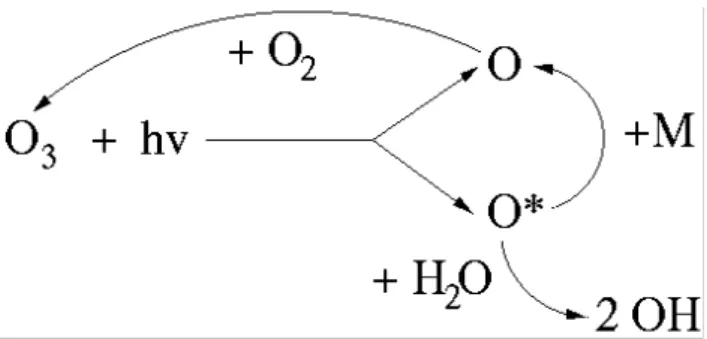
2.3 Processes in the troposphere
Almost all chemical degradation of BVOCs and many other species begin via reaction with the hydroxyl radical, OH. The OH radical is formed during the photolysis of ozone in the presence of water vapour, as illustrated in Fig. 2. Briefly, photolysis of ozone produces an oxygen atom, a proportion of which have sufficient energy to react with water vapour and produce two OH radicals. Some of these high-energy oxygen atoms are quenched via collision with another air molecule (marked as M in Fig. 2) back to a ground state, and reform ozone. The formation of OH is thus principally controlled by the levels of ozone and the flux of radiation.
Other important reactions of BVOCs involve direct oxida-tion by O3and the night-time reaction with the NO3radical.
The NO3 radical is formed during the day, but photolyses
rapidly, and so its levels are usually very low. At the end of the day, reaction of NO2with O3forms NO3in sufficient
levels to oxidise BVOCs. OH also reacts with other impor-tant trace gases such as CO, other VOCs, and CH4. These
reactions may, overall, act as sources or sinks of OH, de-pending on, for example, the levels of NOx. They strongly
control levels of OH (and hence the oxidising capacity of the troposphere) and the CH4lifetime (Crutzen, 1979;
Der-went, 1995; Lelieveld et al., 1998; Pfeiffer et al., 1998; Wang et al., 1998; Sanderson et al., 2003a; Young et al., 2009). Recently, Lelieveld et al. (2008) measured OH levels over a
126 A. Arneth et al.: From biota to chemistry and climate
1
Fig. 2. Production of OH via photolysis of ozone. The photolysis of
ozone (O3)produces oxygen atoms in a ground state (O) or higher energy state (O*); the latter can react with water vapour to produce 2 OH radicals. Some of the higher energy state oxygen atoms are quenched back to the ground state. The ground state atoms reform ozone.
tropical forest and found they were much higher than model predictions. They proposed that HO2 radicals can react
di-rectly with large peroxy radicals produced from VOC degra-dation to produce significant quantities of OH radicals un-der low NOxconditions. A modified version of their
chem-istry scheme including these additional reactions produced OH levels that were in much better agreement with the mea-surements. Aerosols produced from the oxidation of BVOCs can act as cloud condensation nuclei, and surfaces for het-erogeneous reactions (Andreae and Crutzen, 1997; Kulmala, 2003).
Hydrogen is not a greenhouse gas itself, but reacts with OH and so may increase concentrations of CH4 and other
GHGs. The main source of H2is the photolysis of
formalde-hyde (HCHO), produced from the photochemical oxidation of CH4 and VOCs (Price et al., 2007). H2 has small
bio-genic emission sources associated with biological N2fixation
(Price et al., 2007), wetlands (Conrad, 1996) and biomass burning. While reaction with OH removes roughly 20% of atmospheric H2, soil uptake is the dominant sink (Price et
al., 2007), the exact magnitude depending on soil type, mois-ture content and temperamois-ture (Yonemura et al., 2000; Smith-Downey et al., 2006), or snow cover (Rhee et al., 2006). The present day H2soil sink is estimated to be 88±11 Tg H2a−1
by Rhee et al. (2006) who used seasonal and hemispheric variations in H2and D/H isotopic ratios as constraints. Other
estimates range from 40–50 to 90±20 Tg H2a−1(Seiler and
Conrad, 1987; Novelli et al., 1999; Hauglustaine and Ehalt, 2002; Sanderson et al., 2003b; Price et al., 2007) based on measured soil deposition velocities for H2 and estimates of
the global areas of various soil types.
Tropospheric O3is formed during the photochemical
oxi-dation of CO, CH4, and other VOCs in the presence of NOx,
with an additional source from stratosphere-troposphere ex-change (e.g., Stevenson et al., 2006). A recent modelling study by Fiore et al. (2009) has examined the impact of foreign and domestic emissions of NOx, CO and VOCs on
ozone levels in four continental-scale regions in the North-ern Hemisphere. These authors found that the ozone levels in each region were most sensitive to domestic emissions, but transport of ozone and its precursors from foreign regions was also important. The importance of foreign emissions on domestic ozone levels therefore requires a good understand-ing of the terrestrial BVOC and NOxemission patterns (e.g.,
Chameides et al., 1988; Pierce et al., 1998; Wang and Shall-cross, 2000; Sanderson et al., 2003a; Barket Jr. et al., 2004; von Kuhlmann et al., 2004; Folberth et al., 2006; Wu et al., 2007). Wu et al. (2009) showed that the response of ozone levels to changes in emissions of NOx are non-linear
out-side of the summer months, but are linear during summer, when ozone production is limited by NOxlevels. The impact
of clouds on regional tropospheric ozone budgets has been studied by Voulgarakis et al. (2009). These authors showed that cloud cover can reduce OH levels and increase isoprene lifetimes by up to 7%. The largest impacts on ozone lev-els were seen over some marine regions where cloud opti-cal depths are large. High O3 concentrations (40 ppb and
well above) occur during the northern latitude summer across temperate regions of North America, Eurasia and China, co-inciding with the height of the growing season when BVOC emissions, particularly isoprene, are largest. Over tropical regions of India, Amazonia and the Sahel, O3concentrations
peak during the dry season, with biomass burning an impor-tant source of precursors, alongside emissions of NOxfrom
soils (Kirchhoff et al., 1990; Keller et al., 1991). The most important chemical sink for ozone is photolysis in the pres-ence of water vapour). O3also reacts directly with BVOCs
(Bonn and Moortgat, 2003), and dry deposition accounts for approximately 15% of the total O3 loss (Stevenson et al.,
2006). This process is responsible for the low O3levels
ob-served during the night-time when a shallow boundary layer develops. Non-stomatal deposition on land surfaces such as plant cuticles or soil constitutes 30 to 80% of the total de-position sink (Fowler et al., 2001) with surface resistance decreasing with increasing temperature, solar radiation and relative humidity above 60% (Zhang et al., 2002; Coyle et al., 2009).
O3 enters leaves via the stomata; the primary effect of
chronic O3exposure on plants is to reduce photosynthetic
ca-pacity (Ashmore, 2005; Fiscus et al., 2005; Karnosky et al., 2005). However, plants have evolved detoxification mecha-nisms to counter oxidative stress based on enzymes that uti-lize ascorbic acid (Pl¨ochl et al., 2000; Fiscus et al., 2005) or possibly BVOCs (Loreto and Velikova, 2001; Fiscus et al., 2005). Reductions in plant assimilation and increasing main-tenance costs leads to a reduction in the land carbon sink, and thus implies an indirect radiative forcing of ozone on climate (Sitch et al., 2007).
Secondary organic aerosols, formed as the reaction prod-ucts of BVOC oxidation, constitute one of the largest uncer-tainties in the climate system (Forster et al., 2007). SOA affect climate directly by scattering and absorbing radiation,
and act as efficient cloud condensation nuclei (Hartz et al., 2005; VanReken et al., 2005; Dusek et al., 2006). SOA are important for the growth of particles, if not their formation (Hoffmann et al., 1997; Tsigaridis and Kanakidou, 2003; Tunved et al., 2006). Estimates for the present SOA bur-den vary by a factor of five (Tsigaridis et al., 2005). A con-siderable part of this uncertainty relates to the incomplete understanding of the biogenic sources. For instance, until recently oxidation of isoprene was thought to produce neg-ligible amounts of SOA, but recent studies have shown that this is not true (Kroll et al., 2006). Isoprene oxidation is es-timated to produce between 4.6 and 6.2 Tg SOA a−1(Henze and Seinfeld, 2006; Tsigaridis and Kanakidou, 2007). The formation of SOA from biogenic precursors depends on the levels of NOx. For important compounds like isoprene or the
terpene α-pinene, the SOA yield decreased with increasing levels of NOx, whereas the reverse is true for some
sesquiter-penes (Kroll et al., 2005, 2006; Ng et al., 2007).
Ammonia (NH3)has a large agricultural source. Its
reac-tion products (such as NH4NO3and (NH4)2SO4)also form
aerosols which play a key role in cloud formation as cloud condensation nuclei. They provide additional aerosol sur-faces which may scatter incoming solar radiation which will impact on tropospheric photochemistry. A global modelling study by Feng and Penner (2007) showed that 43% of the ni-trate aerosol and 92% of the ammonium aerosols exist in the fine mode which scatters radiation most efficiently. The con-tinuing reductions in anthropogenic emissions of SO2 (the
main source of sulphate aerosols) means that formation of ammonium nitrate will increase in importance (Pye et al., 2009). The interaction of HNO3on aerosols has important
impacts on tropospheric chemistry. For example, the pres-ence of nitrate in aerosols significantly reduces the conver-sion of N2O5to gaseous HNO3(Riemer et al., 2003) which
in turn reduces tropospheric ozone levels (Tie et al., 2003). Overall, SOA formation patterns differ in polluted and clean air environments which will be important to distinguish, e.g., in simulations of preindustrial aerosol burden and concentra-tions of cloud condensation nuclei (Andreae, 2007).
3 Global trace gas exchange modelling
It is evident that surface-atmosphere exchange processes are important for understanding changes in atmospheric compo-sition and radiative forcing from the last glacial maximum to the present day, and for future projections. Biosphere-atmosphere exchange is mediated by physico-chemical and biological processes which are very sensitive to prevailing environmental conditions. Trace gas exchange, ecology, at-mospheric chemistry and climate are associated with pro-cesses that operate in very different characteristic spatial and temporal scales (Fig. 3) and their incorporation pro-vides a challenge to coupled Earth System models. In ad-dition, many interactions may differ depending on whether
a pristine or polluted environment is considered. Until cently, atmospheric chemistry-transport models (CTMs) re-lied on emission inventories which assumed constant sea-sonal or mean-annual emissions over inter-annual to decadal timescales (Prather et al., 2001; Gauss et al., 2006; Steven-son et al., 2006). Coupling CTMs to DGVMs allows the use of emissions which respond to the local climate and surface conditions at high temporal frequencies, as well as a more ac-curate description of dry deposition and uptake of trace gases by vegetation (Hauglustaine et al., 2005).
3.1 DGVM model structure
In the existing DGVMs plant photosynthesis and autotrophic respiration are simulated in relatively similar ways (e.g., based on models by Farquhar et al., 1980; Collatz et al., 1991). Leaf carbon assimilation and water loss are typically coupled as the models contain a representation of the soil water balance, whereby stomatal conductivity and photosyn-thesis are reduced in periods with soil moisture deficit. Au-totrophic and growth respiration are subtracted from gross photosynthesis, and a set of carbon allocation rules deter-mines plant growth. Plant establishment, growth and mor-tality are represented, and their response to resource avail-ability (light, water), disturbance and climate extremes un-derpins simulated population dynamics. Decomposition of dead tissue is described as a function of soil carbon content, temperature and soil moisture. Typically a number of soil pools are distinguished that represent material with different residence times. Some DGVMs have begun to move towards a more detailed representation of canopy dynamics and re-source competition by adopting the “gap model” concept where average individuals represent the properties of a cer-tain age cohort of a given PFT (Moorcroft et al., 2001; Smith et al., 2001). While computationally expensive, the gap con-cept allows the simulation of successional dynamics, reflect-ing competition between light-demandreflect-ing and shade-tolerant plants (Smith et al., 2001; Hickler et al., 2004; Miller et al., 2008). For more detailed review of DGVMs see (Cramer et al., 2001; Prentice et al., 2007; Sitch et al., 2008).
Coupling of the carbon and nitrogen cycles is an active area of research within the terrestrial modelling community (Sokolov et al., 2008; Xu-Ri and Prentice, 2008; Thorn-ton et al., 2009). Many DGVMs assign fixed C:N ratios for plant tissues and assume sufficient leaf nitrogen is avail-able for photosynthesis; only few include a coupled soil C and N scheme (Cramer et al., 2001; Prentice et al., 2007). DGVMs require relatively little input: climate, soil type and atmospheric CO2 concentration and can be run from
(sub)daily to glacial/interglacial time scales. They have been evaluated using flask measurements of CO2 from a global
network of monitoring stations, eddy covariance data of CO2 exchange, field manipulation experiments (e.g.
Free-Air-Carbon Enrichment experiments), and field data on net primary productivity (NPP), biomass and soil carbon content
128 A. Arneth et al.: From biota to chemistry and climate 1
2
Fig. 3. Characteristic spatial and temporal scales associated with DGVMs and climate models, trace-gas biosphere-atmosphere exchange and
atmospheric chemistry. Green lines: processes associated with plant physiology/land cover; yellow lines: trace gas emissions; blue: surface hydrology/energy balance; red: chemical transformations and related processes; grey: weather and climate.
(McGuire et al., 2001; Friend et al., 2007; Hickler et al., 2008).
3.2 Inclusion of new land cover types and processes in DGVMs
3.2.1 Land use, land cover change and related non-CO2
trace gas emissions
A substantial fraction of the anthropogenic emissions of non-CO2trace gas and particulate matter are due to land use and
land cover change (Bruisma, 2003). Already with develop-ment of agriculture some 10 000 years ago (Roberts, 1989) humans began to transform the land surface (Olofsson and Hickler, 2007). Historical land use and cover changes are important not only as a large carbon source over the last centuries (Houghton, 1999, 2003) but for pre-industrial non-CO2 trace gas emissions, e.g., of BVOC and fire related
emissions (Arneth et al., unpublished), and hence for pre-industrial to present-day radiative forcing calculations. In the context of climate change, future land use must both sup-ply agricultural products for a growing population (Vitousek et al., 1986), and target new ecosystem services, like soil carbon sequestration or agrofuels (Lal, 2004). Depending on the crop type and its phenology, future climate warming might be locally either advantageous (increased growing pe-riod) or detrimental (insufficient vernalization, increased wa-ter and heat stress; Lobell et al., 2008) to crop yields. Tropo-spheric O3 tends to reduce photosynthesis and yields
(Ash-more, 2005).
Accounting for the human influence is therefore crucial for modelling terrestrial trace gas exchange and its climate effects through biophysical and biogeochemical feedbacks. In many land use simulations, agriculture is represented as grassland, by harvesting a fraction of the (natural) productiv-ity or crop growing seasons are prescribed (e.g. McGuire et al., 2001; Feddema et al., 2005). Several studies that parame-terised land surface schemes specifically for crops (Challinor et al., 2004; Kothavala et al., 2005; Osborne et al., 2007) have concentrated on short term land-atmosphere interac-tions. The carbon cycle is not closed, and neither the re-moval of carbon through harvest nor the long-term soil car-bon dynamics were analysed. Recent studies (Davin et al., 2007) estimate past and future cooling due to the biophysical effects of anthropogenic land cover change, while Lobell et al. (2006) relate different cooling levels to crop management. Biogeochemical impacts of land use and cover change within DGVMs were simulated initially by replacing forests with productive grassland or simply by harvesting a fraction of the (natural) productivity (McGuire et al., 2001). Us-ing a suite of biogeochemical models, McGuire et al. (2001) found the opposing effects of CO2fertilization and historical
land cover changes to be the two largest factors governing changes in terrestrial carbon storage over the 20th century. Using the DGVM LPJ coupled to the CLIMBER-2 climate model, Brovkin et al. (2004) quantified the effects of histor-ical land cover changes as a biophyshistor-ical (0.26◦C) cooling due to an increase in northern latitude albedo which was par-tially offset by a biogeochemical (0.18◦C) warming due to atmospheric CO2increases over the last 150 years; for future
land cover change, simulations of the biogeochemical warm-ing largely from tropical deforestation either dominated over the biophysical cooling or amplified the biophysical warming associated with Northern Hemisphere land abandonment, de-pending on the socio-economic story-line used (Sitch et al., 2005).
Local-scale crop models have been developed by agronomists since the 1970s and are increasingly being ap-plied at larger scales, projecting an increase in production in the northern latitudes due to CO2fertilization and
warm-ing, while production in the tropical semi-arid areas may de-cline due to water shortage (Rosenzweig et al., 1993; Parry et al., 1999; Reilly and Schimmelpfenning, 1999; Rosenzweig and Iglesias, 2001; Fischer et al., 2002; Tan and Shibasaki, 2003; Challinor et al., 2007). For a regional application, remote sensing information on canopy height was used to constrain carbon stocks and fluxes calculated with a height-resolved vegetation model (Hurtt et al., 2004). The output of crop models is typically restricted to yield and water re-quirements although their internal algorithms often include the crop canopy seasonality. Growth processes of individual crops (or crop functional types), have been implemented as an integral part of the modelling framework in three agro-DGVMs which can be run globally or at the regional scale with the coexisting simulation of natural vegetation (see Ta-ble 1). Generally, progress in this area allows terrestrial bio-geochemical cycle calculations to be explicitly linked with socio-economic scenarios.
In agro-DGVMs, biophysical processes, soil decomposi-tion and some plant physiological processes (e.g. photosyn-thesis and respiration) are computed using the same formu-lations (but with adapted parameters) for crops and natural PFTs. Hence these models compute consistent land car-bon and water budgets for croplands and natural ecosystems. Other parameterizations are crop-specific, such as the phe-nological development and carbon allocation to the different pools (e.g. the economically important yield storage organs) during the growing period. Some functions exist only for managed land, like residue processing, crop rotations or irri-gation. Two different strategies to implement land-use pro-cesses in DGVMs can be distinguished. In the first the pa-rameterizations are built in the host DGVM. For example, algorithms from the EPIC crop growth model (Williams et al., 1989) were adopted in the models Agro-IBIS (Kucharik, 2003) and LPJmL (Sitch et al., 2003; Bondeau et al., 2007). In the second, the DGVM (e.g. ORCHIDEE; Krinner et al., 2005a), is coupled to an agronomy model (e.g. STICS; Bris-son et al., 2002) that provides, on a daily time step, the DGVM with all variables that are crop-specific (Gervois et al., 2004). This approach facilitates fast inclusion of any im-provement in the agronomical representation.
Agro-IBIS has mainly been developed for continental US agriculture (wheat, maize, soybean), and has been intensively tested for the impacts of different management practises on soil and vegetation C and N pools, crop yields, C and water
fluxes, and N leaching. It was applied to investigate crop yields and environmental problems at the river basin scale (Donner et al., 2004; Donner and Kucharik, 2003) and to quantify the various factors associated with farming practices which drive carbon fluxes (Kucharik and Twine, 2007), while Twine et al. (2004) used it to simulate the biophysical effects of land cover change from natural vegetation to crops.
The coupled ORCHIDEE-STICS model has been devel-oped predominantly for European crops with agriculture de-scribed by three generic crop types: wheat-based functions are assumed to represent most of the winter C3-type crops, maize-based parameterizations are used for C4-type crops and soybean-based functions are used for C3-type summer crops. The model has been evaluated against water and car-bon fluxes at specific sites, inter-annual yields at the Euro-pean scale, and is used to simulate the impacts of histori-cal land management on yields and carbon storage in Europe (Gervois et al., 2008) as well as to North American wheat and maize (Gervois et al., 2004).
LPJmL (Bondeau et al., 2007) defines eleven Crop Func-tional Types (CFTs) and one managed grass. It allows trends in global harvest, vegetation and soil carbon, NPP, water and CO2fluxes of the actual vegetation to be simulated and the
impact of land use and land cover change globally to be quan-tified (Bondeau et al., 2007). Zaehle et al. (2007) estimated a carbon sequestration potential of agricultural abandonment and afforestation in Europe of 17–38 TgC a−1 by 2100, al-though this was strongly reduced or even offset by climate warming. M¨uller et al. (2007) produce the inverse picture on the global scale, estimating that the impacts of non-climatic factors on land-use to be as important as the direct climatic factors and CO2fertilisation.
Simulations of the greenhouse gases CH4and N2O, or of
NOx, with Agro-DGVMs have not yet been attempted but
it will be important to assess the impacts of land manage-ment on these emissions. In terms of N2O, important initial
studies have been conducted based on global data assimila-tion (Stehfest and Bouwman, 2006), and by modelling crop production within the ecosystem model DAYCENT (Stehfest et al., 2007) which provides a tool to simulate the impact of agricultural management on soil nitrogen dynamics and trace gas fluxes. At the regional scale, several groups have used GIS data coupled to ecosystem models to simulate GHG ex-change from various land uses, e.g. for rice based agricultural systems in China (Li et al., 2004; Huang et al., 2006), or for grasslands, forests and agricultural systems in Europe or the US (Soussana et al., 2004; Kesik et al., 2005; Del Grosso et al., 2006; Butterbach-Bahl et al., 2008). The next step is to adopt such modules in agro-DGVMs and to analyse the ef-fect of management strategies on emissions reduction, like, for instance, recommended mid-season drainage of rice pad-dies intended to reduce the CH4emissions, or the use of crop
130 A. Arneth et al.: From biota to chemistry and climate
Table 1. Summary overview of three Agro-DGVMs.
DGVM version with crops, land use and land cover change Original DGVM main variables simulated natural PFTs and crops represented and domain of application model tests of the crop sub-module, or of the combined model (natural vegetation + agriculture) applications us-ing the crop sub-modules only
applications using the land cover change sub-modules only (i.e. using a simple land use representation within the original DGVM )
applications using both crop and land cover change sub-modules Agro-IBIS (Kucharik and Brye, 2003) IBIS (Foley et al., 1996) – energy, water, carbon, and momentum bal-ance of the soil-plant-atmosphere system – seasonal LAI – C and N pools, crop yields 8 Tree PFTs, 2 grass PFTs, 2 shrubs PFTs + wheat, maize, soybean (crops for the conti-nental US) – seasonal CO2 and water fluxes at AMERI FLUX eddy covari-ance sites – crop yields and N leaching within the Mis-sissipi basin
– impacts of climate and land use man-agement on crop yields and nitrate export (Donner and Kucharik, 2003; Donner et al., 2004) – impacts of crops manage-ment on NEP (Kucharik and Twine, 2007)
– impact of the land cover change on terrestrial carbon storage (McGuire et al., 2001)
– impact of land use on the energy and water balance (Twine et al., 2004) ORCHIDEE-STICS (Gervois et al., 2004; de Noblet-Ducoudr´e et al., 2004) ORCHIDEE (Krinner et al., 2005b) – energy, water, carbon, and momentum bal-ance of the soil-plant-atmosphere system – seasonal LAI – C and N pools, crop yields 7 Woody PFTs + 2 grass PFTs + wheat, maize and soybean (European crops that have also been shown to be valid for the US) – seasonal CO2and water fluxes at eddy covariance flux sites – national crop yields statistics – seasonal and interannual variability of LAI – comparison against CO2 fluxes from atmospheric measurements – impact of his-torical land cover change on climate (Davin et al., 2007)
– impacts of crop-lands on the Eu-ropean carbon and water budget (de Noblet-Ducoudr´e et al., 2004) – historical impacts of management on yield and carbon storage (Gervois et al., 2008) LPJmL (Bondeau et al., 2007) LPJ (Sitch et al., 2003)
– water and car-bon fluxes of the soil-plant-atmosphere system – seasonal LAI – C pools, crop yields 7 tree PFTs + 2 grass PFTs + temperate and tropical cereals, rice, maize, temper-ate and tropical roots, pulses, sunflowers, groundnuts, rapeseed, grazed or harvested grassland (global) – seasonal CO2 fluxes at eddy covariance flux sites – seasonal simulated fPAR against satellite derived fPAR (globally) – national crops yields statistics for wheat and maize – changes in Soil carbon related to land use changes – comparative impacts of climatic and non-climatic factors on global biogeo-chemical cycles (Muller et al., 2006) – land use and water use modelling (Lotze-Campen et al., 2005) – bottom-up modelling of the NEP anomaly due to the European 2003 heat wave (Vetter et al., 2008; Jung et al., 2008) – impact of the land cover change effects on the ter-restrial carbon stor-age (McGuire et al., 2001)
– historical and future land cover change impact (bio-physical effects and CO2 increase) on
climate (Brovkin et al., 2004;Sitch et al., 2005)
– impact of his-torical land cover change on green water flow (Gerten et al., 2005) – European vulner-ability to climate change (Schr¨oter et al., 2005) – historical impacts of agriculture on the terrestrial car-bon balance (Bon-deau et al., 2007) – estimated impacts of agriculture on the European and global carbon bal-ance for the 21trh century (Zaehle et al., 2007; Muller et al., 2007) – agricultural water consumption & re-lated issues (Rost et al., 2008)
3.2.2 Wetlands and methane emissions
CH4 emissions from wetlands are known to be highly
de-pendent on water table position, temperature and availabil-ity of carbonaceous substrate (Walter et al., 2001). This de-pendence can be seen at both the small (Roulet et al., 1992; Christensen et al., 2003) and the large scale (Bousquet et al., 2006). Similar to natural wetlands, emissions from rice agri-culture are also strongly dependent on temperature (Khalil et al., 1989) and water table as defined by irrigation patterns. Drainage of wetlands leads to a shift to more CO2instead of
CH4emissions, whereas restoration will increase CH4
emis-sions.
Global estimates of present day CH4 emissions from
wetlands are derived either by using process-based models (bottom-up approach, e.g., Cao et al., 1996; Christensen et al., 1996; Walter et al., 2001; Zhuang et al., 2004) or inverse models (top-down approach, e.g. Fung et al., 1991; Mikaloff Fletcher et al., 2004a; Wang et al., 2004; Chen and Prinn, 2006). A large source of uncertainty is in the wetland dis-tribution itself as most processed-based models rely on time-invariant maps of wetland extent. Some process-based mod-els use simplistic empirical relationships between water table depth and CH4oxidation rates and do not represent the
differ-ent CH4transport pathways (Cao et al., 1996; Gedney et al.,
2004). The widely adopted approach of Walter et al. (2001) is based on soil temperature, NPP and the amount of avail-able substrate, and water-tavail-able (derived from a simple hydro-logical scheme) to model emissions. Recent studies (Wania et al., 2010) include a CH4emission model coupled directly
into the DGVM to simulate the interactions between vegeta-tion composivegeta-tion, soil temperature, and water table posivegeta-tion. This approach has the advantage of modelling interactions between hydrology, vegetation and permafrost, which have not been included previously (Cao et al., 1996; Walter et al., 2001).
Methane models are evaluated using site-specific observa-tions from chamber measurements or flux towers. Influen-tial environmental conditions such as water table position, soil temperature or net primary production at the chamber sites can be readily determined for a small sample area and compared to model output. Chamber measurements have the disadvantage of not always including CH4emissions via
ebullition, as these highly irregular emissions are often ex-cluded from data sets. Eddy-covariance flux measurements integrate over diffusion, plant-mediated transport and ebulli-tion (Rinne et al., 2007) in an often heterogeneous flux foot-print that consist of hummocks, hollows and lawns represent-ing very different micro-habitats (Saarnio et al., 1997). In general, DGVMs do not simulate such spatial heterogeneity given their spatial resolution of typically 0.5 to 1 degrees. However, DGVMs can be run for individual sites or differ-ent micro-topographic features. By doing so, they can be used as a tool to explore the impact of small-scale spatial heterogeneity on the simulation of large scale fluxes. Inverse
modelling techniques can help to constrain the process-based models at the regional and global scales. Important limi-tations arise from lack of suitable observations and uncer-tainty in the sink terms, e.g. seen in the large spread in esti-mates of global wetland CH4emissions using this approach,
145–231 Tg CH4a−1 (Forster et al., 2007). Satellite
mea-surements of total column CH4 have also recently become
available (Buchwitz et al., 2005; Frankenberg et al., 2005) and developments in inversion techniques have included us-ing isotopic CH4data (Mikaloff Fletcher et al., 2004a).
Iso-topes of carbon (13C) and hydrogen (deuterium) can help to localise methane sources, but are yet to be included in a global, process-based methane model.
Simulations of past CH4emissions are even more data
lim-ited, especially in the distribution and extent of wetlands for the last glacial maximum and during deglaciation (Kaplan, 2002; Valdes et al., 2005). The inter-hemispheric gradient in atmospheric methane levels derived from ice cores can help locate methane sources in the past. Future wetland emis-sions will depend on warming, directly elevating emission rates and indirectly via changes in the distribution of wet-lands (Cao et al., 1998; Gedney et al., 2004; Zhuang et al., 2004). Zhuang et al. (2004) estimate that high latitude emis-sions have increased over the 20th century and Gedney et al. (2004) predict an approximate doubling of wetlands emis-sions over the 21st century under the IS92A scenario.
Future climate warming is projected to be most pro-nounced over high latitudes, regions where frozen soils are prevalent; especially sensitive are frozen soils that currently exist near the freezing point of water. The spatial and tem-poral dynamics of permafrost and periodic disturbance are crucial in shaping high-latitude landscapes, with important consequences for the spatial extent of wetlands and the ex-change of CO2and CH4. There is increasing evidence that
these changes are already occurring across large portions of the Arctic (Serreze et al., 2002; Hinzman et al., 2005). The active layer depth in permafrost areas is likely to change dra-matically over the next century (Lawrence and Slater, 2005; Euskirchen et al., 2006; Zhang et al., 2008), thus changing local drainage patterns. The thawing of permafrost could lead to better local drainage leading to drier conditions and therefore reduced CH4emissions, but if drainage is impeded,
it may lead to enhanced inundation and wetter and warmer conditions favouring higher CH4 emissions (Christensen et
al., 2004). Permafrost and active-layer dynamics are now being developed and incorporated into DGVMs (Venevsky, 2001; Zhuang et al., 2003; Beer et al., 2007; Wania et al. 2009), and used to investigate the relationship between per-mafrost degradation, wetland-forest carbon dynamics, trace gas emissions and wildfire.
132 A. Arneth et al.: From biota to chemistry and climate
3.2.3 Nitrogen exchange in natural and agricultural ecosystems
Several processes govern the flow of nitrogen through terres-trial ecosystems, including nitrogen fixation; uptake by or-ganisms; immobilisation (assimilation of nitrogen into plant and microbial tissue) and mineralisation (decomposition of soil organic matter to NH+4); nitrification (biological oxida-tion of NH+4 to NO−2 and NO−3), denitrification (biological reduction of NO−3 and NO−2 to gaseous N), and the pertur-bation of the natural cycle by anthropogenic nitrogen depo-sition, and leaching of excess nitrate into groundwater. The division of nitrogen between soil organic matter (C:N∼15) and plant biomass (C:N∼200) together with the total land N budget and the degree to which plants can alter their C:N ra-tios will critically determine the ability of terrestrial ecosys-tems to sequester anthropogenic CO2in the future (Finzi et
al., 2007; Thornton et al., 2007; Gruber and Galloway, 2008). However all of these processes are associated with large un-certainties (Holland et al., 1999; Prentice et al., 2000; Den-tener et al., 2006b). A major uncertainty with regard to the N cycle, the quantification of N2denitrification losses on site
to regional scales, remains an unsolved challenge (Groffman et al., 2009).
At the site scale, a range of process-oriented models with widely varying approaches and degree of detail (Boyer et al., 2006) have been applied with mixed success in natural, semi natural and managed ecosystems to simulate nitrification-denitrification related trace gas emissions. The physico-chemical and biological factors driving nitrification and den-itrification depend strongly on microsite conditions. This poses a major challenge for modelling the temporal dynamic of nitrogen trace gas exchange, and more generally for all redox-sensitive sources (e.g. CH4emission versus oxidation)
since aerobic and anaerobic zones in soils determine whether oxidative processes (such as nitrification) or reductive pro-cesses (such as denitrification) dominate. Simulation of ni-trogen oxide fluxes is further complicated by the need to ac-count for the diffusion resistance of soil and canopy and, for NOx, chemical reactions within the canopy that can alter the
net flux from the soil surface by up to 50% (Ganzeveld et al., 2002a). Single column canopy transfer schemes for NOx
do exist, however, they are yet to be used in conjunction with ecosystem models to simulate nitrogen gas exchanges (Ganzeveld et al., 2002b).
Plot-scale models have been linked to regional databases on soil, land-use and climate to simulate emissions for bo-real, temperate and wet tropical forests (e.g., Kesik et al., 2005; Werner et al., 2007), as well as for agriculturally dom-inated landscapes (Butterbach-Bahl et al., 2004; Gabrielle et al., 2006). However, these upscaling experiments rely heav-ily on the availability and quality of data on soil physical properties (e.g., Batjes, 2002) and initial conditions for soil and vegetation carbon and nitrogen stocks for model
initiali-sation and parameteriinitiali-sation. The latter requirement suggests the potential usefulness of coupling site-scale emission mod-els into DGVMs that provide spatially explicit information corresponding to local climate and pedographic conditions (see for example, Werner et al., 2007).
Several regional and global studies simulated source emis-sions of NOx, N2O (Potter et al., 1996; Potter and Klooster,
1998; Parton et al., 2001) and NH3(Potter et al., 2003) from
soils that were based on process descriptions combined with remote sensing information and vegetation models. At the scale of DGVMs modelling of nitrogen trace gas emissions is still at a very early stage. In general a common structure is applied: N affects gross photosynthesis, transpiration and au-totrophic respiration (Field and Mooney, 1986; Sprugel et al., 1995). N availability to plants thereby controls leaf area and plant growth, with the formation of new tissue being subject to plant specific C:N ratios. Plants retain a fraction of leaf N on leaf abscission and thereby influence the quality of litter entering the soil. This N-dependent quality impacts on the decomposability of fresh litter (Anderson, 1973; Jansens and Luyssaert, 2009). Decomposition of organic matter results in sequestration or release of mineral nitrogen, depending on the C:N ratio of the decomposing material and the N require-ments for the growth of soil microbes. Mineral N dynam-ics usually account for nutrient competition between soil mi-crobes and plants, and processes of leaching to groundwater, including some protection against leaching resulting from adsorption to clay minerals, and a generic loss term to den-itrification dependent on mineral N (e.g. Friend et al., 1997; Thornton et al., 2002). Dickinson et al. (2002) go further by simulating nitrification and denitrification processes as a function of N availability and soil moisture, however, they represent gaseous losses from these processes in a lumped manner.
Recently, algorithms that are based on the adaptation of process-based emission models at the site scale (e.g. DNDC; Li et al., 2000) have been adopted for use in DGVMs (Xu-Ri and Prentice, 2008; Zaehle and Friend, 2009). Taking advan-tage of the “closed” and consistent N cycle formulation of the DGVMs, these approaches tightly couple the terrestrial C and N cycles, and the process representation of N trace gas production and emissions apply (e.g., an empirically derived split of the soil in aerobic and anaerobic fractions). First model integrations have shown global flux estimates to be within the range of observation based estimates (Xu-Ri and Prentice, 2008; Zaehle and Friend, 2009).
Data on nitrogen trace gas fluxes are still scarce (Stehfest and Bouwman, 2006) and often not all information re-quired to correctly interpret these measurements are avail-able. Fluxes are remarkably variable in response to en-vironmental conditions, vegetation type and management practices and despite recent advances in data availability, these differences are not yet fully understood (Schindl-bacher et al., 2004). Site-scale observations of NOx and
temperate/boreal croplands, pastures and forests while infor-mation from tropical and particular semi-arid and seasonally wet regions is in view of the global importance of this biome types still scarce (e.g. Martin et al., 2003; Brummer et al., 2008). Using space-based observations, Jaegle et al. (2004) have recently suggested that soil NOxemissions from
semi-arid regions are significantly contributing to O3
enhance-ment in tropical Africa. A major challenge towards provid-ing a critical benchmark for global scale nitrogen trace gas modelling is the compilation of observations into regional databases, such as in Pilegaard et al. (2006), and in validat-ing and applyvalidat-ing space-based observations, as those derived from GOME or Schiamachy.
N2O concentration observed at atmospheric stations can
be exploited to evaluate the simulated seasonality of net land-atmosphere N2O fluxes using CTMs. These measurements
can then be used in inversion studies to attribute variations in atmospheric concentrations to sinks and sources according to latitudinal bands and terrestrial versus marine origin, which could provide an integrative benchmark of simulated N2O
fluxes (Hirsch et al., 2006). Large uncertainty exists in such inverse estimates, because the assumed prior net N2O flux
is highly uncertain, but potentially important for the inferred outcome (Hirsch et al., 2006). Also, the atmospheric trans-port itself contributes substantially to the observed seasonal cycle of N2O concentrations (Nevison et al., 2007). CTMs
can in principle be also used to evaluate emission of NOxby
transporting simulated emissions to stations with observed nitrogen deposition. However, N deposition estimates from the current generation of CTMs driven with similar emission fields differ considerably because of differences in the repre-sentation of NOxchemistry and deposition processes
(Den-tener et al., 2006b). The potential to use atmospheric data for the evaluation of large-scale NHxemission modelling is
very limited because of the short lifetime of NHxin the
at-mosphere.
First attempts to study climate change feedbacks suggest NO emissions from forest soils in Europe may increase by 9%, whereas N2O emissions may decrease by 6% due to
pre-dicted changes in temperature and rainfall for the 2030s (Ke-sik et al., 2006). Land management dominates site to global-scale N trace gas fluxes. Representing land use in DGVMs (see Sect. 3.2.1) is therefore crucial for modelling N trace gas emissions. Fertilizer application to arable land and pastures have been identified as main drivers of N trace gas emissions, owing to its significant effect on site N availability (Forster et al., 2007). Recently Crutzen et al. (2008) estimated that the loss of N2O from reactive nitrogen (via e.g. fertilization,
N deposition, and indirect emissions in the course of cas-cading) is in the range of 3–5% rather than 2% as used in the IPCC guidelines. This has implications for any land use change from natural towards managed systems and also af-fects our view on benefits which may possibly be achieved by implementing large scale bioenergy production systems as a measure for climate protection. Furthermore, conversion of
natural systems into pasture or arable systems in tropical re-gions or the drainage of wetlands for forestry or agriculture have been shown to result in the mobilisation of soil C and N stocks accompanied by pulses of N trace gas emissions lasting up to several years (e.g., Melillo et al., 2001; Smith and Conen, 2004). Even the change from till towards no-till agricultural systems may promote N2O emissions due to
the alteration of the C and N cycles (Six et al., 2004; Li et al., 2005). Further studies with fully coupled vegetation, cli-mate, hydrology and soil biogeochemical models are needed to gain a comprehensive understanding of possible feedbacks of N trace gas exchange due to global change.
3.2.4 Fire and fire-related emissions
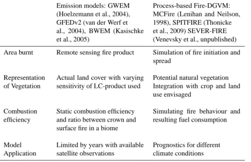
Fire-related trace gas emissions are estimated using global/regional emission models or global, process-based fire models embedded in DGVMs (Table 2). Emission mod-els combine remote sensing products, databases and inven-tories to prescribe area burnt, and to estimate fuel loads in order to predict trace gas emissions. Process-based fire mod-els represent fire initiation, spread and effects. Climate data and ecosystem variables governing fuel load and status (pro-vided by the DGVM) serve as input. Model outputs include area and biomass burnt and associated changes in the sim-ulated carbon pools of vegetation and litter. CO2emissions
are therefore driven by area burnt, fuel load and fuel con-sumption. Both groups of fire models rely on biome-specific emission factors (EF) to estimate trace gas emissions. How-ever, the conditions that determine the ratio between flam-ing and smoulderflam-ing combustion which determines non-CO2
trace gas emissions is fixed (Andreae and Merlet, 2001). Emission models show the influence of extreme fire events and ENSO (van der Werf et al., 2004, 2006) on GHG fluxes to the atmosphere. However, they are limited by the available data-base or satellite information and rely on prescribed as-sumptions about fire behaviour (surface vs. crown fires) and combustion efficiencies. With improving quantity and qual-ity, remote-sensing products are able to capture real time, continuous global coverage but uncertainties remain regard-ing reliable products to estimate area burnt, fuel load (driven by vegetation productivity) and land cover (vegetation type, natural vs. non-natural). Fire Radiative Power is a novel de-velopment, where the energy content of a fire is detected from remote-sensing fire products and can help to distinguish surface from crown fires and possibly combustion complete-ness (Wooster et al., 2005).
Process-based fire models in DGVMs try to capture the bi-directional feedbacks between fire frequency, fire effects and vegetation dynamics. Implementation of fire behaviour and intensity within DGVMs, e.g. the SPITFIRE model (SPread and InTensity of FIRE; Thonicke et al., 2009) in the LPJ-DGVM, provide the basis to simulate trace gas emis-sions. SPITFIRE explicitly accounts for both lightning- and human-caused ignitions. Fire spread only takes place when