Sensitivity analysis of fusion power plant designs using the SYCOMORE system code

HAL Id: cea-02426430

https://hal-cea.archives-ouvertes.fr/cea-02426430

Submitted on 2 Jan 2020

HAL is a multi-disciplinary open access

archive for the deposit and dissemination of

sci-entific research documents, whether they are

pub-lished or not. The documents may come from

teaching and research institutions in France or

abroad, or from public or private research centers.

L’archive ouverte pluridisciplinaire HAL, est

destinée au dépôt et à la diffusion de documents

scientifiques de niveau recherche, publiés ou non,

émanant des établissements d’enseignement et de

recherche français ou étrangers, des laboratoires

publics ou privés.

the SYCOMORE system code

S. Kahn, C. Reux, J.-F Artaud, G Aiello, J.-B Blanchard, J. Bucalossi, S

Dardour, L Di Gallo, D Galassi, F Imbeaux, et al.

To cite this version:

S. Kahn, C. Reux, J.-F Artaud, G Aiello, J.-B Blanchard, et al.. Sensitivity analysis of fusion

power plant designs using the SYCOMORE system code. Nuclear Fusion, 2019, 60 (1), pp.016015.

�10.1088/1741-4326/ab4879�. �cea-02426430�

using the SYCOMORE system code

S. Kahn1_{, C. Reux}1_{, J.-F. Artaud}1_{, G. Aiello}2_{, J.-B.}

Blanchard3, J. Bucalossi1, S. Dardour4, L. Di Gallo1, D. Galassi5, F. Imbeaux1, J.-C. Jaboulay2, M. Owsiak6, N. Piot1, R. Radhakrishnan1, L. Zani1 and the URANIE team

1 CEA, IRFM F-13108 Saint-Paul-Lez-Durance, France

2 CEA-Saclay, DEN, DM2S, SERMA, F-91191 Gif-sur-Yvette, France 3 CEA-Saclay, DEN, STMF, F-91191 Gif-sur-Yvette

4 IAEA, Vienna International Centre, PO Box 100, 1400 Vienna, Austria 5 Aix Marseille Univ, CNRS, Centrale Marseille, M2P2 Marseille, France 6 Poznan Supercomputing and Networking Center; IChb PAS, Noskowskiego 12/14,61-704 Poznan, Poland

E-mail: sebastien.kahn@cea.fr Febuary 2019

Abstract. The next step after ITER is the demonstration of stable electricity

production with a fusion reactor. Key design performances will have to be

met by the corresponding power plant demonstrator (DEMO), fulfilling a large number of constraints. System codes such as SYCOMORE, by simulating all the fusion power plant sub-systems, address those questions. To be able to perform design optimizations, simplified models relying on physical and technological assumptions have to be used, resulting in a large number of input parameters. As these parameters are not always exactly known, the impact of their associated

uncertainties on final design performances has to be evaluated. Sensitivity

methods, by measuring the relative influence of inputs on the figures of merit of the design, allow to select the dominant parameters. This information helps the search for optimal working points, guides the priority for technical improvements and finally allows selecting meaningful inputs for uncertainty propagation. A full set of sensitivity methods and their application on a ITER and a DEMO design will be presented, discussing both the statistical methods behaviors and the physical results. Plasma shape parameters (minor radius and plasma elongations) share half of the net electricity power sensitivity for the DEMO 2015 design while the toroidal magnetic field and the 95 % safety factor are responsible for 23% and 17% of the electric power sensitivity, respectively. The plasma minor radius is responsible for 45% of the pulse duration sensitivity for the DEMO 2015 design, while plasma physics parameters drive ∼ 37% of the pulse duration sensitivity.

1. Introduction

The next step after ITER would be a demonstration power plant (DEMO), producing sustainable electric-ity power. For this purpose, a stable high performance plasma is necessary. To accommodate such extreme condition with the numerous fusion power plant con-straints (plasma facing components protection, super-conducting coil protection, tritium recycling etc ...) in a consistent way, dedicated system codes, aiming to simulate all power plant sub-systems with their inter-actions, are necessary.

The SYCOMORE system code [1], developed at the CEA/IRFM organization, is a set of independent simplified models (modules) communicating through the Integrated Modeling Framework (ITM) data struc-tures. For each module and each loop between mod-ules, the consistency of the design is checked, making sure that only viable designs are retained. The core physics is simulated using the Helios code [2], using the plasma profiles as an input to compute the steady-state power balance. The Scrape-Off Layer (SOL) is mod-elled using an advanced two points model [3], taking into account momentum losses and impurity radiation. As impurity radiation affects both the core and the SOL power balance, a loop between the two cor-responding modules is designed to find the minimal impurity fractions (fImp≡

nImp

ne ) necessary to protect

the divertor targets from both intolerable heat flux per unit of surface (qpeak) and tungsten sputtering

(maxi-mum target plasma temperature Ttargets). This loop,

described in appendix Appendix A, also ensure con-sistent boundary conditions between the SOL and the core plasma. A surrogate model trained on advanced neutronics calculations [4, 5] computes the thickness of the tritium breeding blankets (based on the Helium Cooled Lithium Lead - HCLL technology) necessary to achieve the required Tritium Breeding Ratio (TBR -number of tritium atoms produced per fusion neutron). It also calculates the shield thickness needed to protect the inner leg of the Toroidal Field Coil from excessive neutron flux. The Toroidal Field coil (TF) is mod-elled [6] and the TF width necessary to generate the prescribed magnetic field on plasma axis is deduced. The Central Solenoid (CS) magnet is sized to fit in the remaining space in the centre of the tokamak and is modelled [6] to calculate the generated flux, allowing to estimate the pulse duration [2]. Stresses calculations are performed for both CS and TF magnets to estimate the quantity of steel necessary to hold the stresses gen-erated by the Lorentz forces, providing a coherent ra-dial build for the two magnets. A power conversion module computes the efficiency of the various thermo-dynamical cycles generating electricity from primary

heat [7]. A module then calculates the fraction of tri-tium burnt in the plasma by the fusion reaction [8]. The global power balance of the reactor is finally com-puted to estimate the net electricity power production. As simplified models are used in SYCOMORE, nu-merous assumptions are necessary to define a design. They result in the choice of different scaling laws or model parametrization and can have a great impact on the final power plant design. Reflecting the cur-rent knowledge on the physical and engineering con-strains, these input parameters are not always precisely known. To provide robust designs, those uncertainties must be propagated to the different figures of merit (outputs) used in the design optimization, such as net electricity power production or plasma pulse duration for DEMO. This question can be simply addressed us-ing a Monte-Carlo uncertainty propagation, as it has been done with the PROCESS system code [9, 10, 11]. Such a method, also implemented in SYCOMORE, uses a brute-force exploration of the input phase-space. A large number of power plant designs must thus be evaluated to obtain robust results with respect to sta-tistical uncertainty, reflecting the quality of the input phase-space exploration. As the required number of de-sign evaluations rapidly grow with the dimension of the input phase, only a reduced number of uncertainties sources should be propagated by this method. More general sensitivity analyses are therefore necessary to select the dominant uncertainty sources for the Monte-Carlo uncertainty propagation.

Dedicated algorithms, implemented in the SYCO-MORE code will be presented in section 2. A sensitiv-ity analysis evaluating the relative impact of 6 parame-ters on the ITER design will be presented starting from the ITER design [12, 13]. Finally, a more general sen-sitivity analysis (48 inputs) is performed starting from the DEMO 2015 pulsed design [14] and compared to the initial analysis presented in Ref. [14]. The defini-tion of the variables used in this document are percised in Appendix B.

2. SYCOMORE sensitivity algorithms 2.1. Aim of a sensitivity analysis

In the case of non-linear models, the number of runs necessary for uncertainty propagation or metamodel definition has an exponential dependency on the num-ber of inputs (an additional input adds a dimension for the analysis). SYCOMORE, with more than a hundred inputs and several non-linear models, is not suited for raw uncertainty propagations as it would re-quire a prohibitive number of runs. Sensitivity analy-ses [15, 16], providing a ranking of each input

uncer-tainty contribution to the output ones, help selecting the dominant inputs to perform uncertainty propaga-tions with a smaller input dimension. Such ranking depends on both the range/shape of the input distri-butions (assumptions on the inputs uncertainties) and the model itself (the SYCOMORE code). An interest-ing by-product of some sensitivity analysis methods is the evaluation of the linearity and/or the additivity of the models in the considered range.

A model of the output Y is considered additive when it can be written as

Y = β0+

X

i

fi(Xi)

with β0 a real number, Xi the model inputs

la-belled by the index i and fi an arbitrary function

de-pending only on Xi. If the model contains non-additive

terms, such as XiXj, the influence of Xi on Y depends

on the value of Xj. This effect is defined in this paper

as input interaction, to make a clear distinction with correlations brought by input distributions only. In the SYCOMORE such interactions can typically arise from power laws used to approximate the energy con-finement time or the pedestal electron temperature. As the sensitivity ranks values, the intensity of input in-teraction depends on the input distribution ranges and shapes.

Linear models are a sub-set of the additive models defined as Y = β0+ nX X i=1 βiXi

with βi being a real number (linear coefficients)

associated to the input Xi.

Two different class of methods are considered, following the Occam razor principle:

• linearization methods. If the model is linear, the sensitivity coefficient SRCi can be simply

deduced from their linear coefficients term βi:

SRCi= βi

σXi

σY

with σXi and σY the root mean square (RM S)

associated to the input Xi and the output Y ,

respectively [15, 16]. Therefore, if the output can be fitted with a linear model, the sensitivity ranking is straightforward.

• Global methods. If the output shows non-linear dependencies within the input range, linearization methods are not valid anymore. Global methods,

preserving the model structure, become then necessary. Two types of global methods can be distinguished.

– Screening methods: the output difference associated to the variation of one parameter is estimated on different locations of the input phase-space. This kind of methods needs a small number of runs, but no estimation of the robustness of the results is possible. – Variance methods: based on variance

decom-position, these methods indicates the fraction of variance due to each input or group of in-puts. This allows to define both input sen-sitivity rankings and input interactions in a consistent way, but large number of runs is necessary.

Generally, screening methods are used to select a set of dominant variables to be analysed using variance methods, or regression methods if models are simple enough.

2.2. Sensitivity methods implemented in SYCOMORE The implementation of the sensitivity algorithms is provided by the URANIE statistical framework [17] developed by the CEA. Three sensitivity methods have been selected: the linear/monotonic regression method [18], the Morris method [19] and a pick-and-freeze method for Sobol indexes estimation [20, 21]. 2.2.1. Linear regression method

The linear regression method provides a sensitivity ranking assuming the output has a linear dependency with the inputs. The validity of the linear assumption is tested and statistical uncertainty associated to the ranking coefficient is estimated with indicative, even though not rigorous, 95% confidence levels. More precisely, a set of ns SYCOMORE runs is executed

varying nXinput parameters using a Latin Hypercube

Sampling (LHS) [22] and a matrix A(nS, nX+ 1) is

built. The linear coefficients β = (β0. . . βnX) are

deduced from the output values y = (y0. . . ynS) using

β = (ATA)−1ATy

The Standard Regression Coefficients SRCi used

in the sensitivity ranking, are then defined as

SRCi= βi

s

V ar(Xi)

V ar(Y ).

The outputs are then re-computed using the fitted linear model ˆyi to assert the quality of the regression:

R2_adj = 1 −1 − R2     nS− 1 nS− (1 + nX)    

with R2= 1 − PnS i=1(yi− ˆyi) 2 PnS i=1(yi− ¯yi)2 ¯

yi being the expectation of the sample using the fitted

linear model. The linear regression is invalid if Radj

is low. Another way to verify the linear assumption is to compute the quadratic sum of the SRC coefficients, equal to 1 in case of a linear model. As the input phase-space is randomly sampled, some aspects of the model behaviour can be missed if the number of runs is not large enough to explore the input phase-space. To provide an estimate of this statistical effect, indicative 95% confidence level are computed using a Fisher Z-transform [23].

2.2.2. Monotonic regression method

Ranks can be built with the outputs associating 1 to the lowest output value and nS to the largest

one. Fitting these ranks with a linear regression allow computing the Standard Ranks Regression Coefficients SRRCi, their associated Radj and 95% confidence

levels. Although the theoretical validity of the SRRCi has not been demonstrated, these coefficients

provide indicative sensitivity ranks based on weaker assumptions that the SRCi ones, suitable for more

complex models. 2.2.3. Morris method

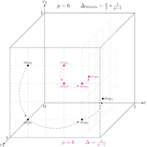
The Morris method [19] is a screening method, providing approximate ranks with a small number of runs and no model assumptions. This method is generally used to identify negligible variables to be removed from more complete sensitivity analysis (Regression or Sobol method). Once the dominant variables are selected, quantitative sensitivity rankings can be provided with associated statistical uncertainties (confidence levels). The principle of the Morris method is to compute the output difference varying only one input. This procedure is repeated r times for each input in different input phase-space regions, capturing the effect of potential non-linearity. Technically, a homogeneous input grid of p intervals is built and r trajectories (replicas) of nX variations are defined with a random

starting point as illustrated in figure 1. Each point of the trajectories is defined iteratively, randomly selecting the next variable to be varied and its variation direction. Once the outputs are computed for all the trajectory points, elementary effects EEt

i are

computed between two neighbouring points: EEti =

y(Xi+ ∆i) − y(Xi)

∆i

Figure 1: Schematic view of two trajectories drawn randomly in the discretized hyper-volume (with a grid containing 6 points) for two different values of the elementary variation ∆.

with i labelling the input Xivaried in a ∆iinterval

(all other inputs remaining the same) and t labelling the random trajectory. Their mean absolute values over all trajectories h|EEi|i = 1_rP

t=r

t=0|EE

t

i| allow to

identify inputs with negligible effects on the outputs and their standard deviation σ(EEi) provides a crude

estimation of their linearity as σ(EEi) = 0 for a linear

model.

2.2.4. Sobol method

Sensitivity indexes [20] can be computed using the notion of conditional variance V ar(Y |Xi = xi)): the

output Y variance obtained fixing one or a group of inputs Xi to a given value xi. The more a variable

is important, the smaller the expected value of the conditional variance E(V ar(Y |Xi)) is compared to the

total variance V ar(Y ). Therefore, the ratio between those two quantities provide a well-defined sensitivity indicator. Normalized sensitivity indexes (Sobol indexes) are defined as Si = 1 −

E(V ar(Y |Xi))

V ar(Y ) and

become, using the total variance theorem V ar(Y ) = E(V ar(Y |Xi)) + V ar(E(Y |Xi)):

Si =

V ar(E(Y |Xi))

V ar(Y )

Two kind of Sobol indexes are generally usually used:

• First order indexes (Sf irst): Sobol index

associ-ated to only one input. Besides providing a sen-sitivity ranking without model assumptions, these indexes provide useful additional information on

the model structure as their sum should be equal to one when the model is additive for instance. Moreover, in the case of a pure linear model they are equivalent to the linear regression coefficients,

as Sf irst,i= SRCi2.

• Total indexes (Stotal): sum of the all the

Sobol indexes defined with input variables groups containing at least the input associated to the total index. If the considered input has no interaction with others in the model, first and total order indexes are equivalent. Their difference brings therefore an estimation of the interaction of each input with all others, providing precious information about the model.

In SYCOMORE, the Sobol indexes are computed using covariance matrices with a pick-and-freeze method based on a covariance matrix estimation [21], that provides an indicative 95% confidence level interval. Such method requires a large number of runs and should be used on a relatively small set of inputs. 2.3. Limitation of the SYCOMORE sensitivity methods

The Morris and the Sobol methods are incompatible with correlated inputs. Linear regression can never-theless be used on this situation and an alternative of the Sobol indexes (Shapley indexes) can be used for non-linear models [24].

The algorithms used to evaluate the Morris and the Sobol indexes fail if any points are removed from their initial samplings. As keeping invalid designs can strongly bias the sensitivity results, these two methods must be used in a range where all designs are valid. A dedicated set of data visualization tools has been set up in SYCOMORE to help the user finding such phase-space. The produced graphics show both the in-valid designs location and their causes (for example pel-lets plasma fuelling impossible or to small radial space available for the toroidal field coils etc..). A better formulation of the model can also significantly reduce the number of un-valid designs. For example, prior to the development of sensitivity analysis in SYCO-MORE, the plasma density averaged electron temper-ature < Te>nwas used as a user input to parametrize

the temperature profile. This led to a large number of invalid design in which the heating power was larger that the power losses. This issue has been solved by adding a loop on < Te>n to determine its minimal

value for a given auxiliary heating power, enforcing the steady-state power balance.

The real impact of several SYCOMORE inputs cannot be captured by the current methods. For

example, the plasma major radius (Rmaj) has a

weak direct impact on plasma performances. But it defines the validity range of the plasma minor radius (amin). As amin has a strong influence on

plasma performances, Rmaj has a strong indirect

impact on performances, which is not captured by the SYCOMORE sensitivity. More generally, threshold effects are not captured by sensitivity methods. Dedicated algorithms can nevertheless be used to quantify threshold/failure effects [25].

3. ITER study

The first sensitivity analysis focuses on key ITER de-sign parameters (inputs) known with large uncertain-ties. These parameters are generally driven by diverse kind of considerations and it is difficult to propose an input probability distribution without a complex study of all the phenomena they reflect. For exam-ple, the energy confinement time enhancement factor (fH) parametrises the scaling law fit uncertainty on

current tokamaks data, but also physics extrapolation to larger scales and the ITER session leader choice on plasma scenario. As such study has not yet been per-formed, no prior knowledge has been assumed for the input distribution (flat shape). The selected inputs for this study are:

• Toroidal magnetic field on axis (BT) :

Technical issues such as defective seals or mechanical fatigue can lead to operate the toroidal field coils (TF) below their nominal performances at BT = 5.3 T for safety reasons. To reflect this

eventuality, BT is varied from 4.0 T (degraded) to

5.3 T (baseline) [12].

• Energy confinement enhancement (fH) :

based on JET experiment, a 20% uncertainty on confinement time is set (0.8< fH <1.2) [26].

Quantitative effects due to the much larger ITER dimension are impossible to predict with current codes, and thus not included in this uncertainty. • Separatrix density parameter (fnsep) :

defined as fnsep =

ne(sep)

fGWnGW, with fGW and nGW

the Greenwald fraction and density respectively, is a key parameter of the SOL two points model. fnsep is varied from 0.3, usually observed in

current tokamaks [26] to a much larger value: 0.9, potentially necessary to protect the ITER divertor [27].

• Heating power (Padd) :

This input defines the necessary heating power to add to the α one, to obtain the steady-state power balance. SYCOMORE does not indicate the necessary power to achieve DT fusion ignition as time dependent simulation of the plasma current and the heating ramp-up must be performed for this purpose (this can be estimated with codes like METIS [28]). The ITER plasma heating will be sheared between neutral beam injection (NBI) providing PN BI =

33 MW and ECRH/ICRH antennas providing 20 MW each, leading to a nominal heating power of PHeat = 73 MW [13]. Potential degradation of

the antenna performances is considered by varying PHeat between 33 MW (NBI only) and 73 MW

(full heating capabilities).

• scrape-off layer width (λq) :

This quantity, defined within larges uncertainties, is varied from the value predicted by the Eich scaling : λq ≈ 1 mm [29], to the very optimistic

value initially taken for the ITER design : λq = 20 mm [30].

• SOL private region spreading factor (Sq) :

this quantity, defined in [31], reflects the divertor energy deposit spreading toward the SOL private region. The two points model describes only the parallel transport while the spreading factor is related to cross-field transport. Therefore this effect is only considered a posteriori on the divertor energy density constrain without affecting the electron temperature at the divertor targets. As large uncertainties are observed on the experimental scaling [29], Sq is conservatively

varied between 1 and 15 mm.

As the IPB98(y,2) confinement time scaling law [32, p2202-2209] is used, H mode is assumed in this study. The variable fL−H = _PM artinPsep

L−H

, with Psep the convected power crossing the separatrix

and PM artin

L−H the H-mode threshold predicted by the

Martin scaling [33], addresses this assumption. As

P_L−HM artin is defined with large uncertainties, no sharp

cut on this variable is applied, replaced by a dedicated sensitivity analysis. In parallel, a sensitivity analysis on fusion power Pf us [2] will be shown to address

the uncertainties on plasma performance. After the ITER working point briefly presented (section 3.1, a sampling will be first used to visualize the fL−H and

Pf us inputs dependency in (section 3.2.1), then a

linear regression method will be used to provide a first sensitivity ranking (section 3.2.2), complemented by the results of a Sobol method (section 3.2.3).

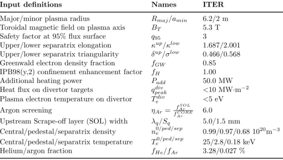
3.1. The ITER working point

The ITER working point is summarized in table 1. Argon impurity is used for divertor protection (beryllium and tungsten impurities from first walls and divertor are neglected). A small electron density profile peaking is assumed ne(0)

ne(ped) = 1.023, allowing

large separatrix electron density values for efficient divertor protection. The upstream SOL width is set at λq = 5 mm corresponding to the values proposed

in the reference [34] and the argon screening set at ηAr =

fSOL

Ar

fcore Ar

= 6 close to the value usually assumed in other system codes such as PROCESS [9, 10]. The separatrix density parameter has been set to achieve a full H-mode following the Martin criteria: fL−H =1.5

with fnsep = 0.7. A good agreement with the ITER

Input definitions Names ITER

Major/minor plasma radius Rmaj/amin 6.2/2 m

Toroidal magnetic field on plasma axis BT 5.3 T

Safety factor at 95% flux surface q95 3

Upper/lower separatrix elongation κup_/κlow _1.687/2.001

Upper/lower separatrix triangularity δup_/σlow _0.466/0.568

Greenwald electron density fraction fGW 0.85

IPB98(y,2) confinement enhancement factor fH 1.00

Additional heating power Padd 50.0 MW

Heat flux on divertor targets q_peakdiv <10 MW·m−2 Plasma electron temperature on divertor T_ediv <5 eV

Argon screening ηAr=

f_ArSOL

fCORE

Ar

6.0

Upstream Scrape-off layer (SOL) width λq/Sq 5.0/1.5 mm

Central/pedestal/separatrix density n0/ped/sepe 0.99/0.97/0.68 1020m−3

Central/pedestal/separatrix temperature Te0/ped/sep 25/2.8/0.18 keV

Helium/argon fraction fHe/fAr 3.28/0.027 %

Table 1: Main Inputs parameters used to define the ITER working point. The parameters in the three last rows are computed by the SYCOMORE system code.

a fusion gain of Q = 9.9 [13] and separatrix densities close to the ones used in SOLPS-ITER codes [27]. 3.2. Results

3.2.1. Data visualization

Before using any sensitivity algorithms, it is interest-ing to visualize the figures of merit dependency with the inputs. A LHS [22] sampling (semi-random sam-pling providing a better repartition than a simple ran-dom sampling) of 5000 design points has been used to explore the inputs phase-space within the ranges pre-sented in section 3. The output values has been sepa-rately projected onto each input Xproj to produce 1D

plots. As all inputs are varied simultaneously, different outputs values can be obtained for a given Xprojvalue.

The corresponding graphics will no longer be a simple line, but will have a width characterized by the corre-sponding conditional variance V ar(Y |Xproj = xproj).

If V ar(Y |Xproj = xproj) << V ar(Y ), Xproj is

domi-nant in the xproj neighborhood. It is interesting to

ob-serve that the mean value of these conditional variance directly defines the Sobol indexes (see section 2.2.4). Projections on more than one variable can also pro-vide a better understanding of input interactions in the model. Figure 2 shows the fL−H (sub-figure 2a) and

Pf us (sub-figure 2b) projection over λq. Lateral left

fL−H and Pf usprojection histograms has been added

helping the visual estimation of V ar(Y ) and the bot-tom histograms shows the λq sampling and the

repar-tition of the failed runs if any. To help the visual-ization of the λq output dependency, the fL−H/Pf us

mean value (dark green horizontal bars) computed on homogeneous λq and its associated uncertainty

(verti-cal dark green bars) is added. Two regimes can be identified :

• low λq : Large λq dependency and small

λq conditional variance (especially for fL−H)

indicating that λqis one of the dominant variables.

• high λq : reduced λq dependency with a larger

conditional variance indicating larger contribution from other inputs.

λq only drives the quantity of argon used to

protect the divertor targets, and hence influence the core through line radiation and D-T fuel dilution. Figure 3a shows the core argon fraction (fcore

Ar )

projected on λq. fArcore decreases with λq with a

much larger slope at low λq than at high λq. This

dependency is similar to the ones observed on fL−H

and Pf us, confirming that fArcoreis a good candidate to

explain the two regimes. Figures 3b and 3c show the power dissipated through argon line radiation (Pline)

in the core plasma and the energy confinement time (τE) projections on λq, respectively. On one hand,

Pline decreases with λq with a much larger slope at

low λq. On the other hand τE strongly decreases

with λq at low λq whereas almost no dependency is

observed at large λq (This behavior is expected as τE∝

< Te>−2.2n [2], < Te>n being the density average

electron temperature of the plasma). The convected power through the separatrix (Psep) naturally decrease

at lower λq while Pline increases. At λq = 2 mm,

[mm] q λ 2 4 6 8 10 12 14 16 18 20 L-H f 0 0.5 1 1.5 2 2.5 3 3.5 (a) fL−H projected on λq [mm] q λ 2 4 6 8 10 12 14 16 18 20 [MW] fus P 0 200 400 600 800 1000 (b) Pf us projected on λq

Figure 2: λq Projection of the L − H transition factor computed using the Martin scaling (left) and the fusion

power (right). All the input of the ITER sensitivity study (BT, fH, fnsep, PN BI, λq and Sq) has been varied

using the ranged detailed in section 3.

[mm] q λ 2 4 6 8 10 12 14 16 18 20 CORE_fAr 0 0.001 0.002 0.003 0.004 0.005 (a) fcore Ar projected on λq [mm] q λ 2 4 6 8 10 12 14 16 18 20 [MW] line P 0 10 20 30 40 50 60 70 (b) Plineprojected on λq [mm] q λ 2 4 6 8 10 12 14 16 18 20 [s] E τ 2 4 6 8 10 12 14 16 18 (c) τE projected on λq [mm] q λ 2 4 6 8 10 12 14 16 18 20 α C 0.65 0.7 0.75 0.8 0.85 0.9 0.95 1 (d) Cα projected on λq Figure 3: fcore

Ar (top left), Pline (top right), τE (bottom left) and Cα (bottom right) obtained with the LHS

the average Psep value (∼ 30). The lower the λq,

the more the plasma cooling is driven by the argon effects, explaining the increased sensitivity of the plasma performances to fcore

Ar (i.e. to λq). Figure 3d

shows the fusion reaction dilution factor Cα projected

on λq. A larger dependency of the dilution effects is

observed at lower λq, where the argon contribution is

larger than the Helium one. This effects amplify the dependency to λq at low values. These two regimes are

taken into account splitting the sensitivity analysis in two λq ranges : [1 − 5] mm and λq[5 − 20] mm.

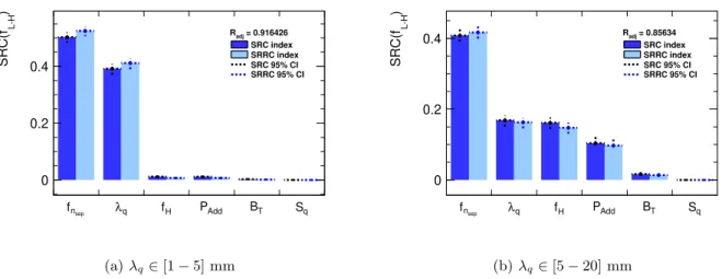
3.2.2. Linear regression results

Figures 4 and 5 shows the fL−H and Pf usstandard

regression coefficients, respectively. These rankings has been evaluated in the λq[1 − 5] mm (left plots) and

λq[5 − 20] mm (right plots) ranges. Both linear (SRC,

dark blue) and monotonous (SRRC, light blue) stan-dard regressions coefficient are shown with their 95% confidences intervals (statistical uncertainties) and the variable Radj, reflecting the quality of the linear fit, is

precised. As Radj > 0.8 for all the linear regression,

their associated rankings are valid. A common fea-ture of all rankings is the negligible Sq contribution.

This result is coherent since the divertor constraint is driven by the plasma temperature at the divertor tar-gets (in the baseline scenario qpeak= 1.8 MW · m−2 for

Ttarget = 5 eV) and Sq does not affects Ttarget in the

two points model.

Figure 4a shows that fL−H is almost entirely

driven by divertor constrains in the low λq regime,

with comparable contribution from separatrix density (SRC(fnsep) = 0.547) and SOL width (SRC(λq) =

0.348). Figure 4b shows that fnsep remains dominant

in λq ∈ [5 − 20] mm, while the λq sensitivity rank is

twice smaller than in λq ∈ [1 − 5] mm. The fH and

Padd contributions become comparable to the λq one,

explaining the variance increase with λq suggested by

figure 2 from section 3.2.1. Almost no contribution from the magnetic field is observed since the plasma performance improvement induced by a BT increase is

counterbalanced by the H-mode threshold increase. The Pf us sensitivity rankings, shown in figure 5,

indicate that the uncertainty associated to the additional power necessary to maintain the steady-state regime is largely dominated by the other inputs. This is explained by the need of larger argon impurity fraction to protect the divertor, that rises in average from 0.07% at for Padd = 33 MW to 0.2% for

Padd = 73 MW. As a consequence, the average line

radiation increases in average from 9 MW to 22 MW between Padd = 33 MW and Padd = 73 MW, while

the D − T fusion dilution factor decreases form 0.89

to 0.85. These two effects counterbalance the gain in performances induced by larger heating power, explaining the marginal Pf us sensitivity to Paddin the

steady-state regime. The divertor constrains have a much stronger contribution at low λq (figure 5a) than

at large λq (figure 5b) with SRC(fnsep) = 0.273

0.280 0.254

in λq ∈ [1 − 5] mm and SRC(fnsep) = 0.072

0.082

0.064 in

λq ∈ [5 − 20] mm. The magnetic field (BT) and the

confinement (fH) contributions are largely dominant

for both ranges. The large BT contribution is expected

as the plasma current (Ip) is inversely proportional

to BT for a fixed q95 value and as Ip strongly drives

the energy confinement (τE ∝ Ip0.96) and the plasma

density limit (nGW ∝ Ip).

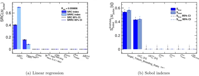
3.2.3. Sobol method results

Some of the linear regression validity coefficients Radj are close to 0.8, suggesting some non-linearities

in the fL−H and Pf usmodels. In this context, it is

in-teresting to compare the SRC/SRRC coefficients with Sobol indexes, computed without linearity assump-tions. The comparison between first and total order Sobol indexes of each input also provides a quantifica-tion of its interacquantifica-tions with the other inputs. Finally, the first order Sobol indexes allow to test the additivity of the models, as their sum should be 1 for an additive model.

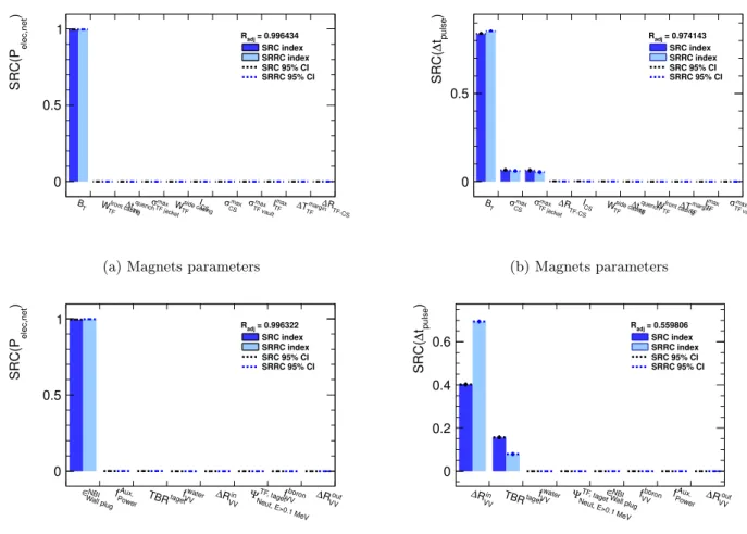
Figure 6 shows the first (Sf irst, dark blue) and

the total (Stotal, light blue) Sobol indexes evaluated

for the fL−H (top) and Pf us(bottom) figures of merits,

in the λq[1 − 5] mm (left) and λq[5 − 20] mm (right)

ranges. The first conclusion is that SRC/SRRC and the first order Sobol indexes are equivalent (within the statistical uncertainties), validating the results shown in section 3.2.2. Even if twice more runs where used for this analysis, larger statistical uncertainties are observed for the Sobol indexes, highlighting the high statistical need of this method. The Stotal indexes are

generally larger than the Sf irst ones, indicating input

interactions in the calculation of fL−H and Pf us. The

inputs that show the largest interactions for fL−H are

fnsep and fH. In the calculation of Pf us, the variables

interactions are shared between the four dominants variables (fnsep, fH, λq and BT).

sep n f λq fH PAdd BT Sq ) L-H SRC(f 0 0.2 0.4 = 0.916426 adj R SRC index SRRC index SRC 95% CI SRRC 95% CI (a) λq∈ [1 − 5] mm sep n f λq fH PAdd BT Sq ) L-H SRC(f 0 0.2 0.4 Radj = 0.85634 SRC index SRRC index SRC 95% CI SRRC 95% CI (b) λq∈ [5 − 20] mm

Figure 4: Sensitivity indexes obtained from a linear (SRC, dark bule) and monotonic (SRRC, light blue) regression of fL−H on the inputs considered in the ITER study, using the variation ranges described in section 3.

The left and the right plots corresponds to the λq[1 − 5] mm and λq[5 − 20] mm ranges, respectively. The vertical

error bars correspond to the 95% Confidence Intervals (CI) estimated using a Fisher Z-transform. The Radj

coefficient, describing the validity level of the linear hypothesis for the model is also precised (result invalidated for Radj < 0.8). T B fn_sep fH λq PAdd Sq ) fus SRC(P 0 0.1 0.2 0.3 = 0.895887 adj R SRC index SRRC index SRC 95% CI SRRC 95% CI (a) λq∈ [1 − 5] mm T B fH fnsep q λ _{PAdd Sq} ) fus SRC(P 0 0.1 0.2 0.3 0.4 Radj = 0.916488 SRC index SRRC index SRC 95% CI SRRC 95% CI (b) λq∈ [5 − 20] mm

Figure 5: Sensitivity indexes obtained from a linear (SRC, dark bule) and monotonic (SRRC, light blue) regression of Pf uson the inputs considered in the ITER study, using the variation ranges described in section 3. The left

and the right plots corresponds to the λq[1 − 5] mm and λq[5 − 20] mm ranges, respectively. The vertical

error bars correspond to the 95% Confidence Intervals (CI) estimated using a Fisher Z-transform. The Radj

coefficient, describing the validity level of the linear hypothesis for the model is also precised (result invalidated for Radj < 0.8).

sep n f λq [mm] PAdd fH BT Sq [mm] ) L-H (f Sobol S 0 0.2 0.4 0.6 S_first total S 95% CI first S 95% CI total S (a) λq∈ [1 − 5] mm sep n f fH λq [mm] PAdd BT Sq [mm] ) L-H (f Sobol S 0 0.2 0.4 first S total S 95% CI first S 95% CI total S (b) λq∈ [5 − 20] mm sep n f BT fH λq [mm] PAdd Sq [mm] ) fus (P Sobol S 0 0.1 0.2 0.3 first S total S 95% CI first S 95% CI total S (c) λq∈ [1 − 5] mm T B fH fnsep λq [mm] PAdd Sq [mm] ) fus (P Sobol S 0 0.2 0.4 first S total S 95% CI first S 95% CI total S (d) λq∈ [5 − 20] mm

Figure 6: First (Sf irst, dark blue) and total (Stotal, light blue) order Sobol indexes for the fL−H (top) and Pf us

(bottom) figures of merit, in the λq[1 − 5] mm (left) and λq[5 − 20] mm (right) ranges. The variation ranges of

the other considered inputs are detailed in section 3. The vertical error bars correspond to the 95% Confidence Intervals (CI) estimated using a Fisher Z-transform.

4. DEMO 1 study

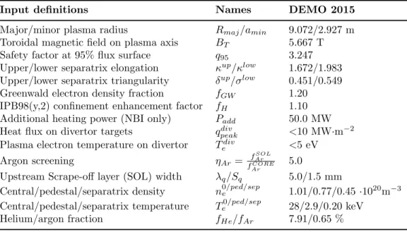
The second sensitivity analysis focuses on the Euro-pean DEMO 2015 [14] pulsed design. The SYCO-MORE inputs used to reproduce it are presented in table 2. To illustrate the potentiality of sensitivity analysis, all the main SYCOMORE inputs (48) are considered. As the uncertainties related to these pa-rameters are not precisely known, a flat ±10% relative uncertainty is set for all inputs, except for Rmaj which

is kept constant for the reasons explained in 2.3. Pa-rameters reflecting physical assumptions and engineer-ing/scenario designs are considered in the same level. Such analysis allows to identify the variables that have the largest influence on the final design, driving the search for better tokamak modelling and technical im-provements. Besides, if the model is linear, the rank of each input can be extrapolated to more realistic uncer-tainty ranges once they are estimated with dedicated analysis. Two effects must nevertheless be checked doing such extrapolation. Non-linear behaviour can appear for larger uncertainty ranges, invalidating the extrapolation. Secondly, if an input is strongly dom-inated by others, the output dependency may appear constant even if it has a non-linear behaviour. Reduc-ing the uncertainty range of the dominant variables may reveal this non-linear behaviour, invalidating the extrapolation of the sensitivity indexes.

As the input phase-space is too large for a global linear regression or a Sobol sensitivity analysis, two steps are considered. First, Linear regressions are performed on sub-groups of 5 to 11 inputs related by their physical meaning, then the final Linear regression/Sobol analysis is performed on the dominant variables from each group. Although a Morris method could have been simply used, this strategy has been chosen for educational purpose as several sub-groups analysis illustrates different features of sensitivity methods. The chosen groups, presented in Appendix B are associated to the plasma shapes (5 variables), the plasma profiles (7 variables), the confinement (8 variables), the scrape-off layer (10 variables), the magnets systems (11 variables) and finally, the tritium breeding ratio, the vacuum vessel and the power balance variables (7 variables). The result of these analyses will be presented with a brief explanation of the physical cause of the ranking and discussion of statistical effects of interest if any. A global ranking will be then shown as a conclusion. 4.1. Sub-groups Results

4.1.1. Plasma shapes

A fair fraction of runs failure is observed (7.8%) on the sampling used to performed the plasma shape lin-ear regression. As a linlin-ear regression can performed on any samplings, this method can be still applied in the presence of invalid designs (this is not the case of the Sobol and the Morris methods). This allows to evaluate the incidence of invalid design removal on sensitivity rankings. A bias can be induced either via input distribution alteration (through σXi), either by

the model dependency (through the linear regression coefficients βi). In this situation, data visualization is

Input definitions Names DEMO 2015 Major/minor plasma radius Rmaj/amin 9.072/2.927 m

Toroidal magnetic field on plasma axis BT 5.667 T

Safety factor at 95% flux surface q95 3.247

Upper/lower separatrix elongation κup_/κlow _1.672/1.983

Upper/lower separatrix triangularity δup_/σlow _0.451/0.549

Greenwald electron density fraction fGW 1.20

IPB98(y,2) confinement enhancement factor fH 1.10

Additional heating power (NBI only) Padd 50.0 MW

Heat flux on divertor targets q_peakdiv <10 MW·m−2 Plasma electron temperature on divertor T_ediv <5 eV

Argon screening ηAr=

f_ArSOL

fCORE

Ar

5.0

Upstream Scrape-off layer (SOL) width λq/Sq 5.0/1.5 mm

Central/pedestal/separatrix density n0/ped/sepe 1.01/0.77/0.45 ·1020m−3

Central/pedestal/separatrix temperature Te0/ped/sep 28/2.9/0.20 keV

Helium/argon fraction fHe/fAr 7.91/0.65 %

Table 2: Main Inputs parameters used to define the DEMO 2015 working point. The parameters in the three last rows are computed by the SYCOMORE system code.

sensitivity ranking if possible.

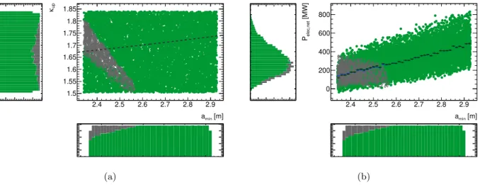
Figure 7a, shows the 2D projection of the run con-vergence status over amin and the upper plasma

sepa-ratrix elongation (κup_{). Full green points corresponds}

to convergent runs and the empty gray diamonds to run failure caused by a too large tritium breeding blankets (BB) thickness (the BB neutronics code is only defined for a given BB thickness in SYCOMORE [5]). The lat-eral histograms show the amin (bottom) and the κup

(left) projection, the green and the gray part corre-sponds to valid design and to design with invalid BB, respectively. A non-valid input phase-space is observed at low amin. In one hand, the bottom histogram from

figure 7a shows that the amin values of the failed

de-signs are mostly far from the central value, decreasing σamin and thus SRC(amin). On the other hand, the

left histogram from figure 7a shows that the κup_values

of the failed designs are mostly close from the central value, increasing σκup and thus SRC(κup).

The right plot of figure 7b shows the projection of the Pelec,net on amin with the Pelec,net (left) and the

amin (bottom) histograms. The Pelec,net mean value

computed in amin homogeneous intervals (horizontal

bars) and its statistical uncertainty (vertical bars) is also shown for convergent (dark green) and all runs, including the invalid ones (dark blue). These profiles allow a visual estimation of the amin linear regression

coefficients (βamin) with and without invalid designs.

Invalid breeding blanket (BB) width will only affect the net electricity production through the BB energy

multiplication factor (Me). As Me is only varying by

∼ 0.1%, only a marginal bias is introduced in the

Pelec,net model. This is coherent with the important

similarities observed between the blue (invalid designs included) and the green (invalid designs excluded) pro-files. Figure 8 shows the linear regression coefficients removing (figure 8b) and keeping (figure 8a) the invalid designs. The linear approximation used for both rank-ings is valid as Radj is well above 0.8. As expected,

keeping the invalid designs increases (decreases) the amin (κup) SRC coefficients by 4.6% (-7.6%). This

effect is much larger than the ∼ 0.1% energy multipli-cation variation and thus, almost entirely due to the input distributions shapes distortion.

The plasma shape variable rankings on Pelec,net

and ∆tpulse shown on figures 9a-9b remain

qualita-tively valid as the number of failed runs is not large enough to modify the ranks hierarchy. Pelec,netis

dom-inated by both amin and κup/low, whereas ∆tpulse is

fully driven by amin. The Pelec,netranking is explained

by the plasma volume and energy confinement time de-pendency with amin and κup/low. The κlow SRC value

is larger than the κup_{one as its baseline value is larger}

(10% variation range represents a larger absolute vari-ation range if the central value is larger, increasing the relative SRC value). The pulse duration is also depen-dent on the remaining space for the Central Solenoid (CS), the larger the CS is, the longer the pulse will be. amin directly drives the CS width, explaining the

[m] min a 2.4 2.5 2.6 2.7 2.8 2.9 up κ 1.5 1.55 1.6 1.65 1.7 1.75 1.8 1.85 (a) [m] min a 2.4 2.5 2.6 2.7 2.8 2.9 [MW] elec,net P 0 200 400 600 800 (b)

Figure 7: Left : 2D projection of the convergence status over κup and amin obtained with the sampling used

for the plasma shape linear regression, with their corresponding 1D lateral histogram projections. The dotted grey line shows reasonability expected elongations as a function of amin [35]. Right: Pelec,net projection over

amin obtained with the same sampling, with their lateral histogram projections. The full green circles (empty

gray diamonds) and the green (gray) histograms corresponds to valid (invalid breeding blanket BB geometry) designs. The dark green (blue) horizontal and vertical lines corresponds to the Pelec,net mean values computed

on regular bins and its statistical uncertainties computed removing (including) the invalid designs, respectively.

min a κ_low κ_up low δ up δ ) elec,net SRC(P 0 0.2 0.4 Radj = 0.970892 SRC index SRRC index SRC 95% CI SRRC 95% CI

(a) Without invalid designs

min a κ_low κ_up low δ up δ ) elec,net SRC(P 0 0.2 0.4 = 0.971199 adj R SRC index SRRC index SRC 95% CI SRRC 95% CI

(b) With invalid designs

Figure 8: Linear (Blue, SRC) and monotonous (Light blue SRRC), standard regression coefficients on Pelec,net

computed on sample where invalid BB design has been removed (left) or kept (right). The errors bars corresponds to the statistical confidence level (CLs) computed using a Fisher Z-transform transform and the Radj corresponds

to the test of the model linearity, both described in section 2.2.1.

4.1.2. Plasma profiles

No invalid designs has been observed for the plasma profiles linear regressions and their linear test coeffi-cient Radjare well above 0.8 (Radj ∈ [0.93 − 0.98]),

val-idating their associated SRC/SRRC rankings shown in figures 9c-9d. Figure 9c shows that Pelec,net is

largely dominated by fGW, as a large average density

value increases the fusion rate and helps the divertor protection (larger plasma separatrix density) simulta-neously. A non-negligible influence from the pedestal

top position (ρped) on Pelec,netis nevertheless observed.

A ±10% variation of ρped corresponds to a variation of

the pedestal width of a factor 18 (from 1% to 18% of amin). Such large variation mainly results from the

parametrization of the code and do not corresponds to a realistic physical result.

Such effects are not present if the input uncertainty ranges are evaluated with realistic values, based on the current knowledge on plasma physics and engineering aspects as done in section 3. The temperature profile

parametrization implies that larger pedestal increases the central temperature for a given average temper-ature. Thanks to this effect the central temperature varies on average from 20 keV at ρped= 0.99 to 37 keV

at ρped = 0.81. As a result, the fusion power varies

from 1800 to 2050 MW, explaining the non-negligible ρped sensitivity ranking. Finally, the Pelec,net

depen-dency on Paddappears to be negligible. A similar effect

as the one discussed in section 3.2.2 is observed : larger heating power (Padd ∈ [45 − 55] MW) increases the

power flowing in the SOL, increasing the argon fraction used to protect the divertor (fAr∈ [0.625 − 0.650] %)

and thus the fusion power through plasma cooling (line radiations (Pline∈ [163 − 168] MW) and fuel dilution

(Cα ∈ [0.522 − 0.525]). The heating power efficiency

(30%) further reduces the beneficial effect of heating power on Pelec,net.

Figure 9d shows the result of the plasma shape variables linear regression on ∆tpulse. ρped appears

to be largely dominant with an almost negligible contribution from fGW. ∆tpulse depends on plasma

profiles through the bootstrap current fraction fBS, the

plasma ramp-up inductive flux consumption Φindand

the vertical flux ΦV F production [2]. An increase of the

pedestal width or fGW will improve the burn duration

through fBSand ΦV F, but will reduce it through Φind.

The results of the ∆tpulsesensitivity analysis show that

this compensation effect limits the contribution from fGW in a stronger way than for ρped.

4.1.3. Confinement

Figures 9e and 9f show the plasma confinement inputs SRC/SRCC rankings. No failed runs and Radj >0.98 is observed, validating the linear regression

results. The left plot shows that Pelec,net is mainly

driven by the safety factor at 95% flux surface (q95). It

is expected as q95is inversely proportional to Ip,

driv-ing both the average electron density and the energy confinement time in a coherent way.

Figure 9f shows the result of the ∆tpulse linear

regression. A weaker q95 dependency is observed,

making the confinement enhancement factor fH (and

Ti/Te in a lesser way) dominant. This result is

expected since the fH and Ti/Te positive impact on

∆tpulse is not counterbalanced by a Ip value increase.

As it is the case for q95, larger Ip increases the need in

CS flux for both ramp-up and flat-top. The Pelec,net

and ∆tpulse rankings both show a negligible argon

screening ηAr = f

SOL Ar

fcore Ar

dependency. This is confirmed by the apparent flat fcore

Ar dependency with ηAr(within

the statistical uncertainties). Two effects potentially explains this behavior : 70% of the line radiation is emitted from the core plasma, it is thus more efficient

to increase fcore

Ar than increasing f SOL

Ar to protect the

divertor. Secondly, smaller fcore

Ar improves the fusion

power. In this situation, larger power must be radiated with argon to protect the divertor targets, increasing the core and SOL average fAr. This effect dumps the

fcore

Ar reduction obtained with larger argon screening.

This effect is confirmed by the increase of the average fSOL

Ar from 2.9% at ηAr = 4.5 to 3.5% at ηAr = 5.5

observed in the sampling used for the linear regression. 4.1.4. Scrape-off layer

Figures 9a and 9b show the SOL variables SRC/SRRC ranks on Pelec,net and ∆tpulse,

respec-tively. In the DEMO baseline design, a relatively large λq is used (5 mm). The divertor constrains

ap-pears to be only driven by the target plasma tem-perature (Ttarget), with a divertor target energy flux

qpeak= 2.73 MW·m−2well below the 5 MW·m−2limit

for Ttarget = 5 eV. Thus, the only variables that are

expected to have an impact on the design are λq, fnsep

and Tmax

target, as the rest of the SOL inputs parametrizes

the SOL power fluxes. fnsepappears to be dominant for

both Pelec,netand ∆tpulseand λq sub-dominant with a

3-4 time lesser contribution. Tmax

target appears to have a

lesser impact. 4.1.5. Magnets

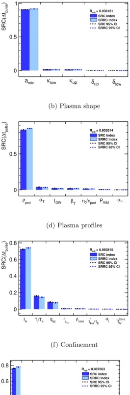
Figures 10a and 10b show the result of the Pelec,net

and ∆tpulse linear regressions on Central Solenoidal

(CS) and Toroidal Field (TF) magnets parameters described in [6], respectively. Pelec,net appears to be

entirely driven by the toroidal magnetic field on plasma axis (BT). This is expected as the rest of the variables

only impact the electricity output though the radial build and magnets design validity parameters. As these effects are only captured through design validity criteria in SYCOMORE, such conventional sensitivity analysis brings no further understanding of the impact of the technical TF/CS characteristics on the net electricity production. Nevertheless, the impact of these parameters on the design can still be roughly evaluated using the Pareto front obtained with the SYCOMORE optimizer mode [8]. Figure 10b shows that BT remains largely dominant for ∆tpulse with

a small contribution of the CS/TF steel stress limit. More resistant steel structures reduces the necessary space by the magnets for a given flux/magnetic field production, leaving space for larger CS supraconductor quantity, resulting in ∆tpulse increase.

4.1.6. Breeding blankets (BB), vacuum vessel (VV) and power conversion group

Sensible tritium breeding ratio (TBR) values for a reactor design lies between 1.07 and 1.10. Hence a 10% variation around the baseline value (1.10) will be out of

the scope the SYCOMORE breeding blanket module was design for. Due to the way the BB module is coupled with SYCOMORE, this validity range triggers invalid designs for TBR > 1.10 and a flat BB thickness dependency with TBR for TBR < 1.07. In order to avoid dealing with invalid design, only a downward variation of the TBR has been considered. The TBR range of variation has not been reduced to keep a consistent relative range of variation with the other inputs, but also as it provides a clear and pedagogical example of a non-linear model, where only the Sobol method is valid.

Figures 10c and 10d show the result of the Pelec,net

and ∆tpulse linear regressions on the BB, VV and

power conversion parameters. Figure 10c shows that

Pelec,net is only driven by the NBI wall plug

effi-ciency since the auxiliary power fraction (fAux

P ower) has

a marginal effect and as other variables only affect

Pelec,net through design validity constrains. On the

other hand, the ∆tpulse linear regression coefficients,

shown in figure 10d are invalid as their associated Radj = 0.56 is well below 0.8.

Figure 11 shows the projection of ∆tpulseover the

target TBR prescribed by the user (T BRtarget_{). As}

ex-pected, two regimes are clearly identified: a flat ∆tpulse

T BRtarget dependency for T BRtarget < 1.07 and a

strong T BRtarget dependency for T BRtarget > 1.07. The flat regime is explained by the minimal BB thick-ness range of the BB module: if the BB width is below it minimal value, the minimal BB thickness is assumed in the design with TBR = 1.07, remov-ing the radial build T BRtarget _{dependency. In the}

1.07 < T BRtarget_{< 1.1 range, the effect of T BR}target

on the radial build, and hence on the CS coil thickness and the pulse duration, is captured as the BB module is well defined for this range of variation.

To obtain a well-defined ∆tpulse sensitivity

rank-ing, the Sobol method is necessary. This method also indicates if the non-linearity arises only from the 1D

∆tpulse dependency (additive model) or from input

interactions. Figure 12 shows the SRC/SRRC (fig-ure 12a) and the Sobol (fig(fig-ure 12b) ∆tpulse sensitivity

of the BB, VV and power conversion inputs. In one hand, large differences are observed between the two

T BRtarget_{sensitivity indexes with SRC(T BR}target_{) =}

0.18 for the linear regression and Sf irst= 0.55 for the

Sobol method. Such differences are expected as the linear fit is largely dominated by the T BRtarget_{< 1.07}

range, representing 86% of the T BRtarget_{input range.}

Thus the points from the T BRtarget_{> 1.07 range will}

be ignored by the linear fit procedure as they have a negligible statistical weight resulting in a small linear coefficient and thus a sensitivity index underestimate.

In the other hand, the two VV width (∆Rin

V V)

sensi-tivity indexes are quite close with SRC(∆Rin

V V) = 0.4

and Sf irst(∆RinV V) = 0.43. The sum of the Sobol

in-dex are close to 1 and the first and the total Sobol indexes are identical within the statistical uncertain-ties. Besides These two observations mean that the

∆tpulse model is additive with respect to T BRtarget

and ∆Rin

V V. As no interaction between T BRtarget and

∆Rin

V V are observed, the linear regression can provide

both a wrong estimate of the ranking (T BRtarget_{) and}

a good one (∆R_{V V}in ). As the model is additive, one would expect the SRC and the SRRC coefficients to be equal, which is not the case. This unexpected be-havior arises from the flat dependency of ∆tpulse with

T BRtarget_{that breaks the monotonicity hypothesis}

as-sumed for SRRC calculation, making the SRRC coef-ficients evaluation ill-defined.

Another strategy to deal with the artificial non-linear ∆tpulse dependency with T BRtarget would be

reduce the T BRtarget _{range of variation to [1.07, 1.10]}

and multiply its SRC coefficient by the ratio of the 10% variation and the [1.07, 1.10] one. Such extrapolation would assume a linear ∆tpulse dependency with

T BRtarget _{on the full 10% variation range. Hence,}

the results of this alternative method would have to be taken with grains of salt.

4.2. Final analysis 4.2.1. Input selection

The SRC ranks and the outputs RM S obtained in the previous sub-group analysis are used to select the inputs for the final sensitivity analysis. If this product of these two quantities is larger than 5%, the associated variable is retained. In decreasing order of importance, the selected inputs are {q95, BT, fGW, amin, κlow, κup}

and {amin, BT, ρped, fH} for Pelec,netand ∆tpulse,

re-spectively. Only two variables (amin, BT) are common

in the initial final selections. amin and BT input has

a contradictory impact on both Pelec,net (positive

ef-fect) and ∆tpulse (negative effect). If the pulse

dura-tion constraint is a strong limiting factor, larger amin

or BT might not be the best way to achieve optimal

DEMO design while other variables such as fH gets

more interesting through their beneficial influence of both ∆tpulse and Pelec,net. Such consideration is well

captured by the SYCOMORE optimizer.

This selection method is blind to cross-groups in-put interactions. If a variable has an important effect through its interactions with other inputs, this selec-tion method might miss an important effect on ∆tpulse

or Pelec,net. To avoid such situation, the selection is

extended using a global Morris analysis. Such method only uses a few points per inputs and hence, its

quan-titative results are not well defined. For example, two identical Morris analysis often provide different sensi-tivity rankings. On the other hand, it is a stable and efficient method to identify negligible inputs or verify the input selection from another method. As the Mor-ris algorithm fails if any run is removed, any BB in-valid designs has been avoided setting the target TBR value to an arbitrary low value. Even though the re-sults are not performed using the same radial build as the baseline design, this analysis remains adapted for an input selection validation. Figures 13a and 13b show the result of these validation studies for Pelec,net

and ∆tpulse, respectively. Although the Morris method

shows consistent results with the initial selection, the {ρped, fnsep} and {

Ti

Te, fnsep, λq} variables shows non

negligible < |EE| > values for Pelec,net and ∆tpulse,

respectively. These variables have been added for the final analysis.

4.2.2. Results discussion

Both amin and κup are varied for the Pelec,net

anal-ysis. Hence a similar BB design invalidity issue as the one discussed in section 4.1.1 is observed. As shown in section 4.1.1, the Pelec,netranking is mostly affected

by the effect of invalid design suppression on input dis-tributions and only a negligible bias will be induced if such designs are kept. For this reason, the invalid BB width designs are not excluded for the Pelec,net

sensi-tivity analysis. Figure 14a shows the result of a Linear regression on Pelec,net using the final extended input

selection. Before discussing the sensitivity rankings in details, a first remark can be made about the input selection: the added variables (ρped and fnsep) shows

the smallest SRC rankings. This validates the initial variable selection method using the products between the SRC indexes and the RM S from the sub-groups.

Among the different input classes, the plasma shape parameters appear to have the largest impact on net electricity production (Pshape

i SRC(Xi) = 0.46),

while the core plasma inputs (confinement and plasma profile parameters) has also a non-negligible influence on net electricity production withPcore pl

i SRC(Xi) =

0.26. The magnet system, has also an important influ-ence with SRC(BT) = 0.21. On the other hand, the

SOL physics inputs influence on steady-state electric-ity production are fond to be almost negligible with SRC(BT) = 0.003. This result may seem

contra-dictory with the important sensitivity to SOL con-strains shown in section 3 (ITER). It can be never-theless explained by the 5 and 19 times smaller un-certainty range used for fnsep and λq, respectively

in the DEMO study. Moreover the DEMO working point is defined for λq = 5 mm and fnsep = 0.6,

which is not in the range where the design is heav-ily dependent to the SOL constraints. On the other hand, the BT uncertainty range is similar for the ITER

and the DEMO study, explaining the much larger BT sensitivity for similar figures of merit (Pf us and

Pelec,net). Considering individual input rank, amin

and BT appears to have the largest (positive)

influ-ence on Pelec,netwith SRC(amin) = SRC(BT) = 0.21.

The (negative) impact of q95remains considerable with

SRC(q95) = 0.17. Thus the potentially necessary q95

increase for plasma disruptions avoidance [36], may have an important influence on net electricity produc-tion. fGW has also a non-negligible contribution to

Pelec,netwith SRC(fGW) = 0.045 as both the core and

the SOL constraints are positively influence by this pa-rameter. On the other hand, fHonly improves the core

confinement and its positive effect is counterbalanced by the need of larger impurity fractions to protect the divertor plates, explaining its absence from the final ranking.

Figure 14b shows the pulse duration final sensi-tivity ranking. As amin is varied, BB invalid designs

are also present for the ∆tpulsefinal sensitivity analysis

(8.1 %). As aminvalue of all the invalid designs is much

lower that the mean amin value, an important bias is

expected if invalid designs are removed from the sensi-tivity analysis and therefore should be kept. Using an arbitrarily small target TBR to avoid invalid BB de-signs should also be avoided as the target TBR drives the BB thickness that influence the CS size and hence

∆tpulse. The best compromise is therefore to keep the

invalid designs even though a (relatively small) bias is expected from the failed runs, as the BB thickness is under-estimated for invalid runs. To estimate the effect of such bias on the final ranking, the linear regression ranking using T BRtarget = 1.1 has been compared to

same one, using T BRtarget = 1.09 containing a much

lesser amount of invalid designs (0.014%). Both rank-ings agrees within the statistical uncertainties, show-ing that keepshow-ing BB invalid designs only introduces a marginal bias on ∆tpulse.

Figure 14b show the final ∆tpulse linear

regres-sion ranking. As for the Pelec,net one, all the input

added after the Morris analysis are dominated by the one initially selected, validating the initial selection. The dominant input is amin with SRC(amin) = 0.45.

amininfluences both the space left to the CS coil

(neg-ative impact on ∆tpulse) and the necessary CS flux for

the plasma current ramp-up and a flat top of a given duration through ΨRU

ind and fBS (positive impact on

∆tpulse). As ∆tpulse decreases with amin, the radial

build effect of amin is dominant. Through their effects

also an important impact on the pulse duration, with a cumulative SRC rank of 0.37.

4.2.3. Comparison with other sensitivity analysis A simpler, but similar study [14] has been per-formed using the P ROCESS system code [9, 10]. Al-though the same outputs are considered (Pelec,netand

∆tpulse), several differences in both of the statistical

method and the tokamak modelling are present. A reduced number of inputs has been a priori selected for the initial P ROCESS analysis, while all the main SY COM ORE inputs has been considered in the anal-ysis presented in section 4, making sure that no sig-nificant effects are missed. Moreover, the inputs vari-ables are varied one at time and hence, interactions are not captured in such analysis. Table 3 from [14, p10] shows the results of the initial DEMO 2015 analysis using P ROCESS. The first remark is that the sensi-tivity on both BT and q95 are not evaluated although

their associated rankings shown in Figure 13a are sig-nificant for Pelec,net. Another difference is the presence

of the helium (cHe) and the tungsten (cW)

concentra-tion in the inputs considered in the P ROCESS sen-sitivity analysis. These two variables are not present in SY COM ORE as the Helium fraction is consistently calculated with the fusion rate, the energy confinement and the ratio between the Helium and the energy con-finement and as tungsten impurity are not considered. For these reasons, only qualitative comparisons should be made between the two analysis.

The dominant input for Pelec,netevaluated by the

P ROCESS analysis appears to be the plasma elon-gation at the 95% flux surface (κ95), driving twice

larger differences that the aspect ratio (A). This re-sult should be compared with the sum of upper and lower elongation SRC indexes, as a 10% variation of the upper/lower elongation only drives a 5% variation on the total one. Therefore, the two analysis quali-tatively agree as Figure 14a shows that SRC(κlow) +

SRC(κup) > SRC(amin). The sub-dominant

parame-ter in the initial DEMO 2015 sensitivity analysis is A. As Rmaj is also fixed for this analysis and A is only

varied by 10% (d( 1

amin) = −damin), such uncertainty

source is equivalent to the aminone. The A sensitivity

is hence coherent with the large amin SRC shown in

Figure 13a. Pelec,netis quite sensible to fGW (referred

as <nli>

nGW in [14]) in both analyses. The main

contra-diction between the two analysis concerns fH(referred

as H in [14]): this paper shows that fHhas a negligible

effect on Pelec,netwhile [14, p10] shows a non-negligible

sensitivity to this parameter. The SY COM ORE re-sult can be explained by the increase of the impurity fraction for divertor protection, inducing more line

ra-diation and D − T fuel dilution. The apparent contra-dictory P ROCESS result potentially results form the different choice of the radiative impurity (Argon for SY COM ORE and Xenon for P ROCESS), the ab-sence of tungsten impurity in SY COM ORE and the difference in the way Helium concentration is treated. In one hand the Xenon and tungsten induces less D −T fuel dilution for a given radiated power, the effect of im-purity seeding increase for divertor protection due to better confinement is lesser in the P ROCESS runs. On the other hand the Helium fraction is fixed in P ROCESS, while the increase of fHe due to larger

Pf us is captured in SY COM ORE. Both effects tend

to reduce the fH improvement effect on Pelec,net in

SY COM ORE with respect to P ROCESS. Neverthe-less, this discussion has to be taken with grains of salts as many other difference are present in both the sensi-tivity analysis and the system codes models (for exam-ple SY COM ORE use an advanced two points model while the SOL physics is only taken into account with a Psep

Rmaj ratio in the P ROCESS DEMO 2015 analysis).

5. Conclusion

The SYCOMORE system code is a modular and co-herent set of modules, simulating the major elements of a fusion reactor. New advanced sensitivity algo-rithms have been recently added allowing to identify the most important engineer/physical parameters for a given figure of merit. This helps the selection of pa-rameters considered in optimization and uncertainty propagation. Sensitivity algorithms bring also pre-cious information about the model (linearity, additiv-ity, variables interactions with others etc...). This can be helpful as compensations effects are often observed in system codes leading to non-intuitive results. A full set of algorithms are implemented: Morris screening, linear/monotonous regression and Sobol method, al-lowing to get meaningful sensitivity rankings for most of the situations. Moreover the Linear/monotonous regression and the Sobol methods provide also confi-dence intervals reflecting the statistical uncertainty on the ranks. This is crucial to prevent from false ranking due to lack of statistics (number of input cases used for the evaluation).

Section 3 presents the test of the new sensitivity tools on the ITER design, using 6 input variables. The intervals used for the variation of the selected inputs have been chosen to reflect known uncertainties on the magnets and plasma performances. The sensitivity of the fusion power (Pf us) and of the L − H threshold

(fL−H) with these inputs has been evaluated using