DEVELOPMENT OF A TOOL FOR
NONLINEAR DYNAMICS
COMPUTATION
Final Project
Internship tutors Dr. Joseph Morlier (ISAE/DMSM)
“Genius is one percent inspiration and ninety-nine percent perspiration.” Thomas Edison
Résumé
La Méthode de la Balance Harmonique est une démarche très attractive pour faire le calcul de la réponse d’un système de vibrations non linéaire. Il est possible d’obtenir un dégrée élevée de précision même si pas beaucoup d’harmoniques sont utilisés pour approximer la valeur de la solution cherchée. De plus, c’est naturel d’éteindre les concepts de la méthode pour évaluer des solutions de systèmes avec plusieurs dégrées de liberté, une fois qu’une approche matricielle est mise en œuvre dans ce modèle, ce qui devient la méthode plus facile à implémenter. Dans ce cadre, la solution issue de la méthode peut être traitée pour trouver un modèle d’identification de paramètres modaux.
Une autre question abordée dans ce travail est comment la Transformée de Hilbert peut être employée pour analyser l’identification modale et pour savoir si le système a un comportement linéaire ou pas. Sur ce sujet, deux méthodes, démarrées par l’article (1) seront mises en examen. La première est la méthode ‘Freevib’, lequel analyse la réponse au cours du temps et est capable d’identifier les paramètres modaux d’un système avec un seul dégrée de liberté libre d’excitations externes. Le deuxième est la méthode ‘Forcevib’, qui agit de façon similaire à la première, mais avec une force d’excitation externe.
Pour conclure, nouvelles techniques d’identification et des idées sont relevées pour l’avenir de telle façon à agrandir les recherches sur des systèmes avec plusieurs dégrées de liberté.
Abstract
The Harmonic Balance Method (HBM) is a way very useful for calculating the response from a nonlinear vibration system. It’s possible to obtain a high degree of accuracy even if few harmonics are used to approximate the required solution. In addition, it’s natural to extend the concepts of that method for evaluating solutions of multi-degree of freedom (MDOF) systems, since a matrix approach is implemented in that model, what becomes the method easier to be dealt with. In that context, the generated solution from this method can be treated to perform a parametric modal identification of a vibration system.
Another topic to be studied in that work is how the Hilbert Transform (HT) can be used to analyze the modal identification and to realize if the system has a linear behavior or not. On that field, two methods, introduced by the article (1) will be investigated. The first one is the ‘Freevib’ method, which analyzes the response through the time and is capable of identify the modal parameters of a single-degree of freedom (SDOF) system free of external excitations. The second is the ‘Forcevib’ method, which does the same thing of the previous one, but with an external excitation.
In the conclusion, new techniques of identification and some ideas for future projects are arisen in order to try to broaden those researches for a MDOF system.
List of Abbreviations
ISAE Institut Supérieur de l’Aéronautique et de l’Espace ITA Instituto Tecnológico de Aeronáutica
HBM Harmonic Balance Method MDOF Multi Degree-of-Freedom SDOF Single Degree-of-Freedom
HT Hilbert Transform
A.D. Anno Domini
IHBM Incremental Harmonic Balance Method EMD Empirical Mode Decomposition
List of Symbols
m Mass
x t Input excitation
y t Response of the system
c Damping coefficient
Non dimensional damping coefficient
k Stiffness coefficient
0 Natural frequency
d Damped natural frequency
Cubic stiffness
X Fourier transform of X
Perturbation coefficient
Contents
1. Overview ... 1
1.1. Introduction ... 1
1.2. Why to study vibrations? ... 2
1.3. Types of systems and methods of evaluation ... 3
1.4. Objectives ... 5
2. Dynamic systems ... 5
2.1. Linear systems ... 5
2.1.1. Time domain ... 6
2.1.2. Frequency domain ... 11
2.1.3. Multi degree of freedom system ... 12
3. Nonlinear systems ... 14
3.1. Perturbation method ... 15
3.1.1. Development of the method ... 15
3.2. The Lindstedt –Poincaré Technique ... 17
3.2.1. Results and analysis ... 19
3.3. Harmonic Balance Method ... 21
3.3.1. Analytical approach ... 22 3.3.2. Numerical approach ... 25 3.3.3. Jump phenomenon ... 29 4. Parametric Identification ... 32 4.1. Hilbert transform ... 32 4.1.1. Introduction ... 32 4.1.2. Definition ... 33 4.1.3. Polar notation ... 35 4.2. Freevib method ... 36 4.3. Forcevib method ... 38
5. Analysis of identification ... 39 6. Conclusion ... 44 7. Bibliography ... 46
List of Figures
Figure 1: World’s first seismograph invented by Zhang Heng, in the Exhibition Hall of
the Museum of Chinese History in Beinjing, China. ... 1
Figure 2: Example of unbalanced wheel ... 2
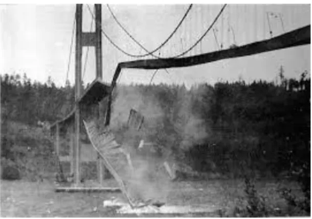
Figure 3: Crash of the bridge due to wind-induced vibrations. ... 2
Figure 4: The Foucault pendulum at the Panthéon of Paris, France, used to show the Earth rotates on its axes. It has a nonlinear behavior for big amplitudes. ... 4
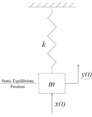
Figure 5: Mass-spring system with one degree of freedom. Adapted from (10). ... 6
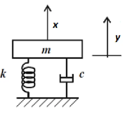
Figure 6: Damped mass-spring system with one degree of freedom. Adapted from (10). ... 7
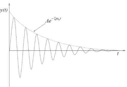
Figure 7: Transient response for a SDOF system with positive damping. Adapted from (10). ... 8
Figure 8: Gain of the system varying with the frequency. Adapted from (10). ... 10
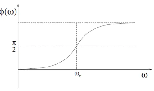
Figure 9: Evolution of phase angle for a SDOF damped forced system. Adapted from (10). ... 11
Figure 10: Variation of the frequency in function of the initial displacement ( 0 1and 1). ... 20
Figure 11: Variation of the frequency in function of the initial displacement ( 0 0.1and 0.1). ... 20
Figure 12: Variation of the amplitude in function of the frequency of the nonlinear system. ... 30
Figure 13: Influence of the amplitude of external force in jump phenomenon. ... 31
Figure 14: Variation of amplitude with decreasing values of frequency c 0.5. ... 31
Figura 15: Complex plan. Adapted from (18). ... 33
Figure 16: Analytic signal in the complex plan. ... 35
Figure 17: The envelope of the analyzed system. ... 40
Figure 18: Instantaneous natural frequency of the studied system. ... 41
Figure 19: The envelope of the second analyzed system. ... 42
Figure 21:The envelope of the third analyzed system. ... 43 Figura 22: Instantaneous natural frequency of the third studied system. ... 43
List of Tables
Table 1: Summary of the modal parameters estimated by the method using Hilbert transforms. ... 44
1. Overview
1.1. Introduction
The human beings were always surrounded by a great number of vibrations. They appear in several places around us, even if we don’t take into account of it, such as every time we hear some sound or in natural phenomena like earthquakes or sea waves. As it’s mentioned by (2), probably the study of vibrations became familiar for ancient civilizations when these people, especially the Greeks, began to produce their first musical instruments, so that the link between music and science started being more natural. By that time, the Chinese had been experiencing a great amount of earthquakes. Thus they had to come up with a way of measuring the quakes’ intensity. Using a mechanism consisting of a system of pendulums, Zhang Heng, a Chinese astronomer, invented the world’s first seismograph in A.D. 132, illustrated by Figure 1. It was capable of recording the time and the direction of occurrence of the earthquake.
Figure 1: World’s first seismograph invented by Zhang Heng, in the Exhibition Hall of the Museum of Chinese History in Beinjing, China.
1.2. Why to study vibrations?
As it was told previously, many processes involve vibrations during their execution. According to (3), our voice is derived from the larynges vibrations with the tongue. Also, the respiratory activity is a result of the oscillatory motion of lungs. Specifically in engineering, lots of problems rolling machines may be generated if it isn’t paid attention with their balance. There may be unexpected consequences of it such as nuisance in urban areas or even an offset of locomotive’s wheels at high speeds (Figure 2).
Figure 2: Example of unbalanced wheel
In addition, vibrations can originate mechanical failures which may result in catastrophic situations. It’s very important to know whether an external excitation in a system can coincide with its natural frequency, because it may lead to an extreme phenomenon called resonance, in which huge deflections are generated, so that failures would be very hazardous. A known example of it was the collapse of Tacoma Narrows Bridge just four months after its inauguration, as it can be seen in Figure 3.
Besides, it can’t be forgotten human beings are usually part of many engineering systems. For instance, when a car is driven, the driver would like to be as comfortable as it can be, without noises and vibrations from the engine. So, it’s also useful to control the transmission of vibrations among different components of a system.
1.3. Types of systems and methods of evaluation
Going further, in a mechanical project of engineering, it’s very important to get under control of the vibration processes of the different materials which a structure is made of. Until the middle of the twentieth century, it was so difficult to evaluate systems from complex engineering problems, since great computer mathematics weren’t bore by the calculators from that time. However, after the 1950s, the use of high-speed digital computers became more usual in terms of treatment of data calculation, making possible to yield solutions based on classical methods with numerical evaluation of terms that cannot be expressed in a closed form. As (4) pointed out, this led the engineering research to develop high-level techniques in which it hadn’t ever been before, because for the first time in ages one was able to carry out huge mathematics with a great amount of accuracy and fast. The pursuit and the need of designing lighter and at the same time resistant structures contributed so much to the improvement of study of mechanical vibrations.
Unfortunately, most progress in dynamical systems that were made throughout the time, since the 1600s when Galileo Galilei (1564-1642) watched the pendulum movement and were amazed by the fact that its period depended on its length (2), considered the systems were linear. Nevertheless, it has been recognized almost all real structures are some kind of nonlinearity (5), either caused by its shape, or by its inertial or material in nature. According to (6), nonlinearity is qualified as being geometric if it comes from large curvatures, resulting in big amplitudes. In case of movable edges, one would find nonlinear inertia effects. In the end, material nonlinearities take place whenever the stress doesn’t vary linearly with the strain.
It’s true that for most purposes regarding the structures as a system with linear behavior is satisfactory, but sometimes it can’t be neglected the nonlinear effects, especially when the system has features which take it to an extreme condition of nonlinearity, such as great external oscillations like the Foucault pendulum (Figure 4). In this context, the works
carried out by Poincaré and Lyapunov at the end of nineteenth century increased significantly the knowledge and improved the research in that area. The French scientist came up with the perturbation method, one of the ways of working out a nonlinear ordinary differential equation, and the Russian one made progress on the foundations of modern stability theory, used in all dynamical systems.
Figure 4: The Foucault pendulum at the Panthéon of Paris, France, used to show the Earth rotates on its axes. It has a nonlinear behavior for big amplitudes.
Other methods were studied with the purpose of yielding a solution of nonlinear systems. One of the most famous is the Harmonic Balance Method (HBM), in which essentially the solution is assumed to have one or at the most two dominant frequency component (7). In case of weak nonlinearities, the HBM is considered the most computationally efficient method for calculating steady-state solutions of such systems.
Nevertheless, if there are big harmonics in the solution of the system, this method produce an innacurate solution at the same time it’s quite complicated to solve the set of necessary equations to reach that solution (8). That’s why (9) proposed a new method more accurate even if the system had strong nonlinearities with multiple harmonics, the Incremented Harmonic Balance Method (IHBM). However, it must be paid attention on implementing this method because it catches the multiples of fundamental harmonics, but neglects possible subharmonics ones.
1.4. Objectives
In this work, it will be seen several methods for calculating the solution of nonlinear systems, examining possible advantages of implementing the Harmonic Balance Method or the Incremental Harmonic Balance Method. After that, techniques of identification of modal parameters will be shown as an example in which the solutions obtained by the previous methods can be useful for engineering projects.
2. Dynamic systems
2.1. Linear systems
As it was mentioned before, great part of structures in the real world take part of a nonlinear dynamic system. However, before tackling this kind of system, it’s really recommended the mathematical definition and the physical concept beyond of the meaning of what would be a linear system is well assimilated.
One consequence of having a linear system is that it follows the principle of superposition. From (10), it can be stated as:
“If a system in a initial condition S1 y1 0 ,y1 0 responds to an inputx t1 with an output y t1 and in a separate test an input x t2 to the system initially in state
2 2 0 , 2 0
S y y produces an output y t2 then the superposition holds if and only if the input x t1 x t2 to the system in initial state S3 y1 0 y2 0 , y1 0 y2 0
results in the output y t1 y t2 for all constants , and all pairs of inputs x t1 ,
2
x t .”
The principle of superposition is important because it can be applied in both static and dynamic way to verify the total response of the system in terms of time or frequency domain analysis. In practice, however, this principle isn’t a good test for linearity since it will be required infinite tests with all possible values of , ,x t1 e x t2 . On the other hand if
2.1.1. Time domain
The simplest system that can be modeled in the study of vibrations is the mass-spring one, as indicated in Figure 5.
Figure 5: Mass-spring system with one degree of freedom. Adapted from (10).
This system can be easily analyzed by means of Newton’s second law, yielding the equation:
my ky x t (2.1)
In equation (2.1), one can find the mass m , the stiffness k and one external excitation
x t . If there aren’t external forces, the system is called unforced and a free motion is observed. Looking for non-trivial solutions specifying initial conditions y 0 A and
0 0
y , it’s found the following result:
cos n
y t A t (2.2)
In equation (2.2), the parameter n is the natural frequency of free oscillations due to the fact it would be the frequency which the system would vibrate with indefinitely. Therefore, as it isn’t possible thanks to the validity of thermodynamic constraints (10), there must exist some mechanism of dissipation of energy. From that, it’s introduced the damping
coefficient in (2.1), so that the system becomes represented by Figure 6 and described by equation (2.3).
Figure 6: Damped mass-spring system with one degree of freedom. Adapted from (10).
my cy ky x t (2.3)
Once again, if the interest is evaluate the non-trivial solutions for the damped system provided of free motion of Figure 6 with initial conditions y 0 A andy 0 0, one will
arrive at (2.4): cos nt t d y t Ae t (2.4) In which 2 c mk (2.5) 1 2 2 1 d n (2.6)
The factors indicated by (2.5) and (2.6) are respectively the damping ratio and the damped natural frequency. From the analysis of (2.4) and (2.6), one can notice the damping ratio must be positive; otherwise the response of the system would be unbounded. If 1, there will not be oscillations, and the system will tend asymptotically from the initial condition to zero. Similar situation would be found if 1, the system being non oscillatory but coming back to its equilibrium. Finally, if 0 1, the oscillations will decay exponentially. That’s why the solution (2.4) is also known as the transient solution, once it disappears as time goes on, as one can appreciate in Figure 7.
Figure 7: Transient response for a SDOF system with positive damping. Adapted from (10).
Now if it’s considered a forced system, by Fourier analysis, the external signal may put in the form of Fourier series, regarding to the periodic part of excitation, with one single frequency of excitation , so that the system can be modeled by (2.7):
cos
my cy ky X t (2.7)
The solution of equation (2.7) will be composed by two parts (2.8): the homogenous one, which it’s already been calculated and is expressed by (2.4), and the particular one, which must be defined by inspection.
t s
y t y t y t (2.8)
In linear systems, the particular solution won’t be dependent of initial conditions and will persist as time goes on as well even if there is not the transient solution anymore. For this reason, it’s called steady-state solution. Besides, it must be periodic and consist of the same frequency of the external excitation, but not necessarily in phase with it. So, a nice guess for the steady-state solution of (2.7) would be:
cos
s
y t Y t (2.9)
In order to obtain the amplitude Y and the phase angle , one can substitute (2.9) in (2.7) and separating the coefficients of sin and cos, giving:
2 cos
m Y kY X (2.10)
sin
Eliminating the sin and cos from (2.10) and (2.11), yields to: 2 2 2 2 1 Y X m k c (2.12)
Before analyzing equation (2.12), one can rewrite it in function of the natural frequency and of the damping ratio, in order to study what happens if the external frequency is modified which gives:
2 2 2 2 2 2 1 4 n n Y X m (2.13)
Looking into equation (2.13), it is easy to show that equation has a maximum value when the frequency obeys the relation (2.14):
2 2 1 2 2
n (2.14)
When it happens, we say r, called resonance frequency. It corresponds to the maximum amplitude the system can reach, and its value is very important in terms of designing and conception of an engineering project. In the Figure 8, it is illustrated the response of a SDOF system considering only the steady-state solution.
Figure 8: Gain of the system varying with the frequency. Adapted from (10).
From the equations (2.10) and (2.11), it is also possible to know how the phase angle changes if the external frequency is modified, obtaining the relation:
2 2 2
tan n
n
(2.15)
Figure 9: Evolution of phase angle for a SDOF damped forced system. Adapted from (10).
One can notice in Figure 9, there is a change of phase when the frequency is greater than the value of resonance.
If one gathers the functions (2.13) and (2.15) as part of a complex functionH ,
with amplitude represented by (2.13) and phase angle equal to (2.15), this complex function will be called FRF (Frequency Response Function). One should also realize that for linear systems this function doesn’t depend on the amplitude of excitation, so that it is quite useful way to discover if a system is linear or not.
2.1.2. Frequency domain
In this section, it’s going to be notice there is another way of solving a SDOF system with an input y t and output x t like the previous section and determining its FRF function. For it, it will be employed the Fourier transformation, which is defined by the integral (2.16):
i t
G F g t e g t dt (2.16)
With the Fourier transform, the input and output signals of the system discussed have frequency-domain representations, what make possible to set up a link from X to Y .
For that, one can take the Fourier transform given by (2.16) of both sides of the equation (2.3), which describes the SDOF system analyzed, generating the relation (2.17):
2
m ic k Y X (2.17)
So, the FRF can be made explicit directly by means of the evaluation of the Fourier transform calculated (equation (2.18)).
2 1
H
k m ic (2.18)
Or still, in terms of n and :
2 1 1 2 n n H i (2.19)
From (2.19), it can be seen that a system is determined if its modal parameters n and are defined.
2.1.3. Multi degree of freedom system
In order to treat the notion of a system that has many degrees of freedom (MDOF), one can generalize what was seen in the previous sections. According to (4), one system of that type with n degrees of freedom can be described by the following relation:
i t
M y C y K y F e (2.20)
Where in (2.20), M is the matrix n x n of mass, C is the matrix n x n of damping, K is the matrix n x n of stiffness and F is the vector n x 1 of external forces applied to the system.
As the matrices M , C and K are symmetric and have inverse, there is a theorem
from Algebra Linear theory which assures the existence of an orthogonal matrix , which owns your rows formed by the eigenvectors of the system MDOF, so that:
y z
Therefore, if the equation (2.20) is multiplied on the right by T
, this relation becomes:
T T T T i t
The new terms generated from this operation represented by the equations (2.22), (2.23) and (2.24) are called modal parameters and are diagonal matrices.
T d M M (2.22) T d C C (2.23) T d K K (2.24)
This yields to a decoupled system of equations, becoming easier to evaluate it for each degree of freedom labeled i, according to the relations for:
i t
i i i i
m z c z k z p e (2.25)
Where pi is a generalized force component. If pi is zero, their solutions for each degree of freedom is similar to (2.9):
sin
i nit
i i di i
z Ae (2.26)
In which Ai and i are defined by the initial conditions of the problem and i is the modal damping ratio and ni is the th
i modal natural frequency, described by the respective
relations (2.27) and (2.28). 2 i i i i c m k (2.27) 2 1 di ni i (2.28)
Coming back to the initial problem’s variables, it’s obtained:
1 sin i i n t i ij j di i j y t A e t
In case there are non-null forces, it’s interesting to develop the solution in the frequency domain. As an analogously manner as it was done in (2.17), one can define a modal FRF for each SDOF from decoupled MDOF system in modal coordinates. So, the th
i modal FRF will be: 2 1 i i i i G m ic k (2.29)
U G P (2.30)
With G diag G1 ,...,Gn .
So, substituting (2.30) into the equation of the motion, the relation (2.31) is found:
T
H G (2.31)
Writing each element of H , one can explicit the FRF functions for any process
i j
y y , given for the transfer functions:
2 2 1 2 n ij ij k nk k nk kA H i (2.32) Where ik jk ij ik jk k kA m (2.33)
Are the residues or modal constants.
It’s really important to do some remarks about these methods of solution, especially related to nonlinear systems. As is pointed out by (10), nonlinearity has destructive effects on modal analyses, since the last relies on principle of superposition, which generally doesn’t hold for nonlinear systems. Also, the decoupling properties for linear systems in modal variables is lost if one have a nonlinear system. Thus it’s indispensable to figure out other techniques for calculating specifically nonlinear systems, what it will be showed in next sections of this work.
3. Nonlinear systems
In search of solutions for nonlinear systems, some methods will be carried out focusing on the calculating of Duffing equation (3.1), which arises in many cases of oscillators whose stiffness don’t follow Hooke’s law.
3 cos
3.1. Perturbation method
3.1.1. Development of the method
The method developed here is generally used when nonlinearity is small. In other words, when the coefficient is near zero (11). In order to examine systems which present weak nonlinearities, they can be expressed by the general equation (3.2).
2
u u f u (3.2)
One can think of this equation as a family of ordinary differential equations, if the scaling parameter is in the interval 0 1. If 0one fall into the linear case for instance. The goal of this method is to try to find all periodic solutions in the form of power series of (12). So, let’s suppose there is a periodic solution u t of period T. It can’t be forgotten that periodic solutions are being sought. That’s the reason a solution like (3.3) cannot be guessed.
2
0 1 2 ...
u t u t u t u t (3.3)
If it so, non-periodic terms like cos , sin2
t t t t would take part of the solution, what
isn’t admissible. However, this feature can be prevented if the period T is expanded in terms of . 2 1 2 2 1 ... T h h (3.4)
Providing a variable t change in (3.2) and substituting (3.4) on it, yields to the
new equation of the system, that admits a periodic solution u of constant period 2 :
2 2
2 2
1 2 2 1 2
1 ... 1 ...
u h h u h h f u (3.5)
In which the dashes represent differentiation with respect to . Now it may be assumed as solution the time series (3.6):
2
0 1 2 ...
u u u u (3.6)
Substituting relation (3.6) into (3.5), expanding f u in Taylor series and grouping the coefficients of power of , a set of linear differential equations is generated.
0 0 0 u u (3.7) 1 1 2 1 0 1 u u h u (3.8) 2 2 2 2 2 1 0 2 u u h h u (3.9) ... And so on, where functions are equal to:
0 1 2 f u t (3.10) 1 0 1 0 2 2 1 1 2 2 u f u h f u t h u (3.11) ...
To solve these equations the initial conditions are supposed to be:
0 0 , k 1 0 0, k 0 0, for 0,1,...
u a u u k (3.12)
The general solution for equation (3.7) is:
0 cos
u a (3.13)
In order to solve (3.8), the relation (3.10) is expanded in terms of Fourier series, after substituting it on (3.8), yielding to:
1 1 1 10 11 1
2
2 cos cos kcos
k
u u h a C C C k (3.14)
Since there are no secular terms presented in the solution, the expression 1 11
2h a C 0 must hold for all . Consequently,
11 1 2 C h a (3.15)
So, the general solution of (3.14), after having taking into account the initial conditions is:
1
1 10 2
2
1 cos cos cos
1 k k C u C k k (3.16)
After that, this process is repeated as many times as one want, until an acceptable solution is reached. In each step, the function will be equal to:
0 1 2 cos cos m m m mk k C C C k (3.17)
The periodic condition (3.18) must hold for all the domain of the problem:
11 1 1 2 2... 2 m m m C h h h h h a (3.18) Leading to the th m - equation to be solved: 0 2 cos m m m mk k u u C C k (3.19)
So that, at the end, the solution is obtained:
0 2
2
1 cos cos cos
1 mk m m k C u C k k (3.20)
According to (12), even though the method seems to be great, it always good to remember every step ahead it’s given throughout the solution, this method just introduces small corrections of second order or higher, making it very laborious for tiny variations in the final response.
3.2. The Lindstedt –Poincaré Technique
In this technique, the nonlinear dependence of the frequency on the nonlinearity is taken into account. For this, the frequency of the system is exhibited explicitly by means of the following transformation (3.21):
t (3.21)
With it, the independent variable of the system is changed, using the chain rule and becomes:
2 3 0
u u u (3.22)
In equation (3.22), the prime indicates the derivative with respect to . Now the variables and u are exhibited as unknowns of the system. Then, solutions can be sought by requiring the expansion of and u.
0 1 ...
u u u (3.23)
1
1 ... (3.24)
Substituting (3.23) and (3.24) in (3.22) and separating the coefficients of 0
and 1 yields to, respectively:
0 0 0
u u (3.25)
3
1 1 0 2 1 0
u u u u (3.26)
The first equation (3.25) has the general solution (3.27):
0 cos
u a (3.27)
Where and are constants. So, the relation (3.26) becomes: 3 3
1 1 cos 2 1 cos
u u a a (3.28)
Or if the equation (3.28) is rearranged, it becomes:
3 3 1 1 1 3 1 2 cos cos 3 3 4 4 u u a a a (3.29)
Whose particular solution is:
3 3 1 1 1 3 1 2 sin cos 3 3 2 4 32 u a a a (3.30)
One can notice there is a secular term in the solution found (3.30), which would lead the system to a non-periodic solution. As periodic solutions are being sought, the coefficient of this term must be eliminated. That is:
3 1 3 2 0 4 a a (3.31)
Then, combining the result from (3.30) and (3.23), the solution of the equation (3.22) is found: 3 1 cos cos 3 3 ... 32 u a a (3.32)
Where its associated natural frequency is:
2
3
1 ...
If it’s remembered that t : 2 3 2 3 1 3 cos 1 cos 3 1 3 ... 8 32 8 u a a t a a t (3.34)
3.2.1. Results and analysis
Then, let’s solve the equation (3.35) just for an example.
2 2
1 0
u u u (3.35)
Its initial conditions are u 0 a 0, 0u 0, where , and are constants.a
If one approximation of third order is carried out to solve (3.35), the solution will have the form:
2 3
0 1 2 3
u u u u u (3.36)
Evaluating the method using the previous approach will result in:
3 3 5
3 7
cos cos3 cos cos5 24cos3 23cos
32 1024
4cos 7 104cos5 2115cos3 2015cos
98304
a a
u a
a
Also, the period of the response can be made explicit:
2 2 4 3 6 3 21 81 1 8 256 2048 a a a (3.37)
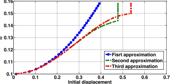
The equation (3.37) is the third order approximation for the frequency of the system. If one stops at the previous approximations (first and second), it would be possible to analyze if the solutions converge. To illustrate that, in the Figure 10, with a natural frequency of 0 1 and a cubic stiffness of 1, the results for frequency are evaluated for these first approximations.
Figure 10: Variation of the frequency in function of the initial displacement ( 0 1and 1 ). Then, the same thing is made, but now with a natural frequency 0 0.1 and a cubic stiffness equal to 0.1. The results can be appreciated in the Figure 11:
Figure 11: Variation of the frequency in function of the initial displacement ( 0 0.1 and
0.1).
In the Figure 11, it’s possible to see that the second and the third approximation diverge. If we remember that the following relation holds:
2 0 (3.38) 0 0.2 0.4 0.6 0.8 1 1.2 1.4 1 1.1 1.2 1.3 1.4 Initial displacement Fisrt approximation Second approximation Third approximation 0 0.1 0.2 0.3 0.4 0.5 0.6 0.7 0.1 0.11 0.12 0.13 0.14 0.15 0.16 Initial displacement Fisrt approximation Second approximation Third approximation
We notice the value of epsilon is increasing in fact. So, the method starts to diverge, since there aren’t small perturbations anymore.
To overcome it, one method similar to the Lindstedt –Poincaré technique was developed, basing on a different way of representing the perturbation. Instead of the previous equation (3.38), one expands the frequency as (3.39):
2 2 0 1 n i i i e (3.39)
Doing that, the parameter of perturbation stays in the same order of the natural frequency and the cubic stiffness (4).
3.3. Harmonic Balance Method
By continuing the idea of the previous methods discussed, if one searches some kind of periodic solutions for nonlinear systems, certainly it can be sought in the form of Fourier series. Nevertheless, how it’s impossible to make considerations with infinite terms, the general solution is approximated by finite sums of trigonometric functions:
0 cos sin n i i i u t A i t B i t (3.40)
The procedure for evaluating the solution starts with the replacement of (3.40) the relation into the differential equation of the problem. After that, the trigonometric products and powers arisen from the expansion of (3.40) are replaced by harmonics sums and balanced, so that the harmonic coefficients of both sides of the resulting equation are the equal. Each harmonic yields to a nonlinear equation that can be solved by an iterative method like Newton-Raphson to determine the coefficients of the approximated solution.
For getting a good approximation, one should consider the type of non-linearity involved in the system, bearing in mind, for instance, even power expansion terms generate even harmonics with a constant term, and odd power expansion terms yield to odd harmonics. So, the cubic linearity requires only the odd harmonics, whereas the quadratic non-linearity needs all harmonics. In problems with free vibrations or forced vibrations without damping, the approximated solution must have just one of the trigonometric function (sin or cos) (13). Just in case of forced damped systems these terms must be presents or to add a phase angle on each harmonic:
0 1 sin n i i i x t c c i t (3.41)
3.3.1. Analytical approach
So, to show how the process is, one takes once again the Duffing’s equation, representing a free vibration system:
2 3
0 0
x x x (3.42)
The following solution (3.43) will be proposed for getting the response of the system:
1cos 3cos3
x t c t c t (3.43)
Replacing the value of (3.43) into (3.42), expanding the trigonometric powers and joining only the present harmonics that belong to approximated solution, one system of two unknowns are obtained:
2 2 2 3 2 1 0 1 1 3 1 1 3 3 3 3 0 4 4 2 c c c c c c c (3.44) 2 2 2 3 3 3 0 3 1 3 1 3 3 1 3 9 0 2 4 4 c c c c c c (3.45)
If one considers an initial condition likex0 c1 c3, and substitutes it on equations (3.44) and (3.45), there will be just c3 and as parameters to be determined.
2 2 2 2 2 2 2 3 3 0 0 3 0 0 3 3 0 3 0 0 3 9 3 3 0 2 4 2 4 c x c x c c x c x x (3.46) 2 2 2 2 2 2 3 3 0 3 0 0 3 3 0 3 0 0 9 3 1 9 2 0 4 4 4 c c x c c x c x x (3.47)
For calculating the result of the problem, one has to work out the system composed of the relations (3.46) and (3.47) computationally.
After, the same thing may be done, if it’s considered a forced system, like indicated by the relation, instead of one with free vibrations.
2 3
0 sin
x x x F t (3.48)
If one harmonic is admitted as an approximated solution, i.e.x t c1sin t, and
2 2 3 3
1 0 1 1 1
1 3
sin sin sin 3 sin sin 0
4 4
c t c t c t c t F t (3.49)
In order to hold the equality, it’s necessary that:
3 2 2
1 0 1
3
0
4 c c F (3.50)
By equation (3.50), it’s noticed it’s the behavior of a nonlinear resonance, in which may exist until three real roots. (colocar aqui o fenomeno do jumping).
Another way of evaluating a nonlinear solution is by means of a variation of Harmonic Balance method called Incremental Harmonic Balance (IHB), developed by (9). First of all, one expands the general solution by using Taylor series before the substitution of the approximated one. For example, the forced damped system represented by relation (3.51) is taken:
2 2
0 0
2 cos 0
x x x F (3.51)
Where the prime indicates the derivative in respect to and t. So, carrying out
this expression around 0 yields to (3.52):
0 x x x F
x x x F (3.52)
In which 2 2
0 x 2 0 x 0x Fcos . Adopting the simplest solution for (3.51), one has: 1 1 1 1 1 1 1 1 1 1 1 1 sin cos cos sin sin cos sin cos cos sin sin cos x c d x c d x c d x c d x c d x c d (3.53)
Substituting the equations (3.53) into the expression (3.52) and eliminating the harmonics, the following equations are obtained:
2 2 3 3 1 1 1 0 1 1 1 1 0 1 0 1 2 2 2 1 1 1 1 0 1 0 1 1 1 2 2 2 0 1 1 1 1 1 0 3 3 3 3 2 2 4 4 4 9 3 2 2 2 4 4 3 2 0 4 c d d c c d c c c c c d c d d c c c c d c d (3.54) 2 2 2 3 1 1 1 1 0 1 1 1 1 1 1 3 2 2 1 1 1 0 1 0 1 0 1 1 2 2 2 0 1 1 0 1 1 3 9 3 3 2 4 4 4 2 3 3 3 2 2 4 4 4 2 0 c d d d d d d c d c F d c d c d c d c d d d (3.55)
If we remember that , and F are constant, , F and are also constants
and can be eliminated from (3.54) and (3.55), resulting in the system represented under the form of matrix: 2 2 2 2 1 1 0 1 1 0 1 2 2 2 2 1 1 1 0 1 1 0 3 2 2 2 1 0 1 1 0 1 1 1 2 3 2 2 1 1 1 0 1 1 0 1 3 3 3 2 4 2 3 3 2 3 2 4 3 3 2 4 4 3 3 2 4 4 c d c d c d c d c d c d c c c d c d d F c d d (3.56)
Firstly, one attributes values to c1 and d1 what leads to the solution of the system (3.56) and new values of c1 and d1 are found. This process is repeated until that
1 0 and d1 0
c . When it happens, one will have found the solution c1 and d1for the parameters , , and F 0. Sometimes, there will be critical points on the curve which don’t converge. In order to avoid these cases, the arc length is used, having the resonance as a control parameter.
2 2
2 2
1 c1 c1 d1 d1 1 1 r (3.57)
In which c d1, and 1 correspond to the last solution evaluated. If we expand the relation (3.57) in Taylor series, we’ll have;
2 2 2 2 1 1 1 1 1 1 1 1 1 1 1 2 2 2 2 2 2 c c d d r c c c d d d (3.58)
Then, the relation is added on the system, resulting in:
1 1 0 1 1 1 1 0 1 1 1 10 1 10 1 0 3 2 2 2 1 0 1 1 0 1 1 1 2 3 2 2 1 1 1 0 1 1 0 1 2 2 2 2 1 10 1 10 0 3 2 2 2 3 2 2 2 2 2 2 2 2 2 3 3 2 4 4 3 3 2 4 4 a c d c c c d b d d c c d d c d c c c d c d d F c d d c c d d r (3.59) Where 2 2 2 2 1 1 0 2 2 2 2 1 1 0 9 3 4 4 3 9 4 4 a c d b c d (3.60)
3.3.2. Numerical approach
In the previous examples, the Harmonic Balance method was implemented considering one degree of freedom. In addition the methods of evaluation may be tedious and laborious if the required approximation has to be quite refined (7). So, following the approach performed by (14), it will be seen how it’s possible to make the method interactive and feasible to implement through a computational environment, extending the idea for any degrees of freedom.
Firstly, the system with n degrees of freedom can be represented by the relation:
3 0 1
cos
sin
M
C
K
L l l l lx
x
x
x
f
f
l t
g
l t
(3.61)Where M, C and Kl are matrix n x n. Once again, the sought solutions are the ones
that are periodic. So, its response may be expressed approximately by M term harmonic Fourier series, in which Mh > L, so that:
M 0 1 cos sin h k k k x t a a k t b k t (3.62)
The next steps are:
Divide the time period for analysis of the response into N number equals intervals of size dt T N, remarking the fact that the Nyquist criterion must be satisfied
Carry out x t at the times x 0 , x t , 2x t ,..., x N 1 t for the
whole period of the signal
For M harmonic terms, and one degree of freedom the equation (3.61) can be written by the system (3.63):
0 1 1 0 2 . . 1 1 1 0 . 1 0
1 cos sin . cos M sin M
1 cos 2 sin 2 . cos M 2 sin M
. . . .
. . . .
1 cos 1 sin 1 . cos M 1 sin M 1
. h h h h h h M M x x t x t x N t t t t t t t t t N t N t N t N t a a b a b (3.63)
This system can be represented in a compact form X A. At the beginning, the
vector A is guessed.
The nonlinear terms are evaluated for the results obtained from the precedent step in time domain:
0 . . 1 h h t H h x t h N t (3.64)
And by means of the procedure known as Alternating Frequency/Time Domain, firstly carried out by (7), it’s possible to get their coefficients of their representation in Fourier series; 0 1 cos sin N k k k h t q q k t r k t (3.65)
Finally, substituting all that relations (3.63), (3.64) and the correspondent coefficients from the Fourier series of the external force F, yields to the system (3.66): 0 0 0 1 2 1 1 1 2 1 1 2 2 . . . . . 0 . . . . . . . . . 0 L h h M M L M M h h f a q f a q g b r f a q g b r K 0 0 0 0 K M C 0 0 0 C K M 0 0 0 0 K M M MM C 0 0 0 MM C K M M (3.66)
Or in a reduced form YA Q Fe 0. The goal of the system (3.66) is to find the coefficients a a a b0, , , ,..., 1 0 1 aM, and bMthat satisfy the system above. It’s important to watch as well that each row of the system is a function of those coefficients, i.e.:
0, , ,...,1 1 , 0, for 1, 2,..., 2 1
i M M
The easiest way to work out it is to evaluate Newton-Raphson method, in which an initial set of values is guessed. For this, it’s performed a Taylor series around this point, so that: 00 10 10 0 0 00 10 10 0 0 00 10 10 0 0 0 1 1 00 10 10 0 0 0 1 0 , , ,..., , 1 , , ,..., , , , ,..., , , , ,..., , , , ,..., , ... ... i M M i M M i i i M M a a b a b a a b a b a a b a b f a a b a b f a a b a b f f f a a b a a b M M M M M M (3.68)
If nt 2Mh 1 and higher order terms are neglected, the system (3.66) may be rewritten as: 1 1 1 1 0 1 1 1 10 0 2 20 1 0 0 1 1 . . . . . . . . . . . . . . . M nt nt nt nt nt nt M M f f f f a a b b f f a f f a f f f f f f b a a b b (3.69)
This can be taken asFi F0i J Ai i, where is the vector of coefficients of the solution. The force on the system is the sum of linear forces YAi, the nonlinear forces Qi and the external forces Fei. Y is the Jacobian part of the linear part and “i” is the suffix which denotes the iteration number. At the end of the iteration, the net force is:
i i i ei
F YA Q F (3.70)
The Jacobian related to (3.70) can be calculated at every step by: 1 T T F Q J Y Q H A A (3.71) Where 1 0 0 . 0 0 0 . 0 0 . . . . . 0 0 . . 0 0 0 . 0 1 T T h h t Q A h N t (3.72)
Guess a set of initial Fourier coefficient A. Solve it for Aiwhich makes 0 i F in equation (3.70), i.e., 1 0 i i i A J F ;
Set new values for coefficients in iteration as Ai 1 Ai Ai;
Calculate Fiand verify if Fi < tolerance, in which Fi : max Fi ;
If the above condition is valid, computation stops, otherwise repeat the above process until the tolerance value reaches its condition. The final set A gives the coefficients of periodic solution.
3.3.3. Jump phenomenon
One curious thing that may happen in a nonlinear system is the jump phenomenon. In this section, it will be demonstrated by using the harmonic balance method.
A harmonic forced damped system governed by the relation (3.73) is used for the following examples:
3 cos
mx cx kx x F t (3.73)
Adopting the harmonic balance method, we’ll find a solution by using an approximation with one harmonic i.e.:
cos sin
x t a t b t (3.74)
Taking the expression (3.74), replacing the value of the solution in (3.73) and eliminating the higher order terms, yields to the system (3.75);
2 3 2 2 3 2 3 0 4 3 0 4 a k m bc a ab ac b k m b ba F (3.75)
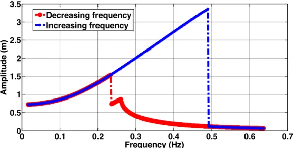
Then, to obtain the solution of the equation (3.73), one must work out the nonlinear system (3.75) in terms of a and b. The Figure 12 illustrates that solution for the parameters
1, 0.1, 1 and 1
Figure 12: Variation of the amplitude in function of the frequency of the nonlinear system.
The first thing on can notice is the abrupt discontinuity in both curves. On the blue curve, as the frequency increases, the amplitude follows this behavior, until it drops abruptly. Similar behavior can be watched in respect to the red curve, this time in another sense. As the frequency decreases, the amplitude increases, until it changes so fast to a greater value of amplitude.
This is called jump phenomenon and it comes from the fact that for some values of frequency there will be until three possible values for the amplitude, as we can see by inspection of the real possible solutions of the system (3.75).
This phenomenon is a characteristic of many nonlinear physical systems, reflected in the Duffing equation as well. To attenuate this feature, one can vary the amplitude of the external force as it’s drawn in Figure 13:
0 0.1 0.2 0.3 0.4 0.5 0.6 0.7 0 0.5 1 1.5 2 2.5 3 3.5 Frequency (Hz) A m p li tu d e (m ) Decreasing frequency Increasing frequency
Figure 13: Influence of the amplitude of external force in jump phenomenon.
Seeing the curves in Figure 13, it’s possible to observe that the smaller is the value of the external force, the weaker is the jump phenomenon, for increasing values of frequency.
To conclude this section, it’s also important to know the effect of the sign of the system stiffness. In other words, to know what happens whether we have a hardening system or a softener one. In we see the effect of this cubic parameter .
Figure 14: Variation of amplitude with decreasing values of frequency c 0.5.
In the Figure 14, we can realize that the inclination of the curve has changed as well as with the reducing of the cubic stiffness, the jump phenomenon is still damped.
0 0.1 0.2 0.3 0.4 0.5 0.6 0.7 0 0.5 1 1.5 2 2.5 3 3.5 Frequency (Hz) A m p li tu d e (m ) F = 0.1 F = 0.5 F = 1 0 0.1 0.2 0.3 0.4 0.5 0.6 0.7 0 0.5 1 1.5 2 2.5 3 Frequency (Hz) A m p li tu d e (m ) = -1 = -0.1
4. Parametric Identification
In this part of work, one is interested in obtaining the unknown parameters of the model of a system from the input-output information.
There are two sorts of approaches in order to come up with the identification problem. If it’s known which equation the system has as a model, the only thing to do is to carry out the unknown parameters of the system. This way for making the identification is called parametric identification. However, there are some situations in which not even the governing equations of the structure system is available. This problem is known as non-parametric identification. The latter one is clearly more difficult to be evaluated than the former, since there is no even evidence about what kind of problem one is dealing with.
The theory of linear system identification is well developed, but more and more nonlinear there have been presented in engineering projects, so that new techniques of nonlinear identification have been developed throughout the years. Various researches have been done to investigate the nonlinear vibratory identification feature (15), (16). Some applied the principle of harmonic balance for the identification of multi degrees-of-freedom systems (17). Nevertheless, this method has encountered some difficulties especially with respect to numerical features of these systems.
In this section, an approach by using Hilbert transforms will be employed for carrying out parametric and non-parametric identifications of nonlinear systems.
4.1. Hilbert transform
4.1.1. Introduction
Integral transforms are very important on developing techniques in physics systems, since with them one can change the domain of study to another one more convenient to develop some theory. With the Fourier transform, for instance, it’s possible to move from a time to frequency domain depending on the circumstances. In this section, the another integral transform, the Hilbert transform, meaningful for the identification of dynamical systems, will be tackled.
4.1.2. Definition
To understand on what one talks about, it’s necessary to define a bi-dimensional plan with coordinates t, . Let’s take D as one domain of this plan, with each point , a complex number, belonging to D. So, it’s defined a complex function z , with z D , such that:
, , ,
z t u t jv t (4.1)
In which u t, and v t, are complex functions and 2 1
j .
The function given by (4.1) is said to be analytic in D if, and only if, u t, and ,
v t are continuous and can be differentiate in the whole domain D. So, taking a point z0 inside a neighborhood C D, such that z0 is analytical in C, according with Cauchy
theorem, (18), it follows: 0 0 1 2 z z dz j z z (4.2)
One calls a signal to be analytical, if it can be represented by a complex function with real variable t in the form:
,0 ,0
t u t jv t (4.3)
So, if the relation (4.3) is compared with the definition (4.1), the analytical signal is just the value of an analytical function z0 through the real axe t.
It can be demonstrated that the line integral along a semi-circle with radius R, Figura 15, when R , is an analytical signal (18). In other words:
0 0 1 2 t t P dt j t t (4.4)
Where P is the principal value of Cauchy. Thus, if one takes the equation (4.3) with the relation (4.4), it can be written that:
0 0 0 1 2 u t jv t u t jv t P dt j t t (4.5)
If the real part is separated from the imaginary one of the expression (4.5), it yields to
0 0 v t P u t dt t t (4.6) And 0 0 u t P v t dt t t (4.7)
Where each of one of the integrals (4.6) and (4.7) are defined as Hilbert pairs. It follows that the Hilbert transform and its inverse are defined respectively as (4.8) and (4.9):
u P H u t v t d t (4.8) And 1 0 v P H v t u t d t (4.9)
In these equations, u t and v t are real functions. Just to feel how this mathematical
tool works, let’s carry out the Hilbert transform of a harmonic signal with constant frequency: cos u t t (4.10) So, cos cos P sin H t v t d t t (4.11)
Therefore, one can notice this transform produces an offset of -90° in the signal phase, with the response in the same domain.
4.1.3. Polar notation
An analytical signal has a geometrical representation in the form of a phasor rotating in the complex plane, as illustrated by Figure 16:
Figure 16: Analytic signal in the complex plan.
A phasor is a vector at the origin of the complex plane having length, called envelope as well,A t , and an angle t . So, it’s possible to represent the analytic signal in its trigonometric form:
cos sin j t
X t X t t j t A t e (4.12)
In this way, we’ll have:
cos
u t A t t (4.13)
And
sin
v t A t t (4.14)
2 2
A t u t v t (4.15)
And its instantaneous phase:
1 tan v t
t
u t (4.16)
If one takes the derivative of (4.16) related to time, it will be obtained the instantaneous natural frequency t :
2 2
d t u t v t v t u t
t
dt u t v t (4.17)
With the relations (4.15), (4.16) and (4.17), one can build up a signal and with the concept of phasor, to get the amplitude, the phase and the frequency, instantaneously, of whatever signal it there can be and to determine if one system is linear or not.
4.2. Freevib method
Now, it will be presented a technique first introduced by (1). It consists in doing a signal processing analysis of vibration systems, linear or not, in order to get the characteristics of these oscillatory systems.
The method will be performed, by taking an example of a SDOF system with viscous damping and writing the governing differential equation:
0
my t c A y t k A y (4.18)
In which c A and k A are respectively the damping coefficient and the stiffness in function of the amplitude. One can divide the equation (4.18) by the mass and to obtain the relation (4.19): 2 0 0 2 0 y h A y A y (4.19) Where 0 2 c A h A
m is related to the viscous damping characteristics, and 2
0
k A A
m is the undamped natural frequency of the system, and y t is the dynamic
are signals with non-overlapping spectra and h t is lowpass with y t highpass, such as
and
H h t y t h t H y t H y y (1), it’s possible to apply the Hilbert transform
in both sides of the equation (4.19), so that; 2
0 0
2 0
y t h y y (4.20)
Multiplying the relation (4.20) by j, 2 1
j , and adding it to equation (4.19), yields to:
2
0 0
2 0
Y h A Y A Y (4.21)
The relation (4.21) is the analytical function of the system, i.e.
j t
Y t y t jy t A t e , with A t y t 2 y t 2 and t tan 1 y t
y t . The
function y t is the Hilbert transform of the system, A t is the envelope and t , the instantaneous phase. It’s important to remark both 2
0 2
0 t and h0 h t0 are functions of time.
Then, the first and second derivatives are taken and substituted in equation (4.21), obtaining the equation for free vibration analysis:
2 2
0 2 0 2 2 0 0
A A A
Y h j h
A A A (4.22)
Avoiding trivial solutions Y 0, the real and imaginary parts in the brackets must be zero: 2 2 0 2 0 0 A A h A A (4.23) 0 2A 2h 0 A (4.24)
One can thereby write expressions for the instantaneous modal parameters, natural frequency and damping coefficient, depending on the derivatives of the envelope and the instantaneous frequency: 2 2 2 0 2 2 A A A t A A A (4.25)
0
2
A h t
A (4.26)
So, with the equations (4.25) and (4.26) with the relations (4.15) and (4.17), it’s possible to evaluate the modal parameters evolution through the time if the amplitude y t
and its Hilbert transform y t are known. In addition, the restoring force f As and damping
force fd A presented in the system can be carried out by means of the equations (4.27) (10): 2 0 d s f A A Ah A f A A A (4.27)
4.3. Forcevib method
In the previous section, on was interested in calculating parameters data from a free vibrations system. However, in practical life, performing a method capable of handling modal analysis of nonlinear systems with an input signal excitation would be very useful.
Having it in mind, a method named ‘Forcevib’ was presented by (19). For this, the same approach in the precedent section is done, with the difference that one can now represent the external excitation by its analytical signal form as it follows:
2 0 0 2 Y h A Y A Y X m (4.28) Where now j t x
X t A t e is the force in analytical form. Evaluating the same
process done before, the equation for forced vibration is obtained:
2 2
0 2 0 2 2 0
A A A
Y h j h X t m
A A A (4.29)
Splitting up the relation (4.29) into real and imaginary parts, after some algebraic manipulation, yields to;
2 2 0 2 2 t t A A A A t t m A m A A A (4.30) 0 2 2 t A h t m A (4.31)
In which t Re X t Y t , t Im X t Y t are real and imaginary
parts of input and output ratio signals according the relation:
2 2 2 2
X t x t y t x t y t x t y t x t y t
t j t j
Y t y t y t y t y t (4.32)
And x t and x t is the force vibration and its Hilbert transform respectively. Like is pointed out by (19), equations (4.30) and (4.31) are general form compared to relations (4.25) and (4.26), since the latter reduce to the former if there’s no excitation forces
0
t t . Besides, according to (19), expressions (4.30) and (4.31) have more
robustness, as a result of the presence of the first and second derivatives of the signal envelope and instantaneous frequency, determining modal parameters even under complicated test conditions, such as when excitation is a non-stationary quasi-harmonic signal with a high sweep frequency.
To work out equations (4.30) and (4.31), it’s necessary the value of the mass, which is unknown a priori. To deal with this problem, a modal mass value must be defined. As in the majority of the cases, the mass is constant and the natural frequency doesn’t vary along the time, eliminating that frequency from (4.30), one defines the modal mass as:
2 2 2 A A m A A A A A A (4.33)
And the operator denotes the deviation of the corresponding functions in the numerator and denominator during time t. So, making a plot of the values of the numerator
by the values of the denominator, the mass will be the slope angle of straight line for a linear sdof system. If there are lots available data, the least square method can be performed for the mass value calculation (19).
5. Analysis of identification
In order to assure the efficacy of determining the modal parameters, one software was developed with the guide MatLab interface, adapting the source code from Michael Feldman
of Faculty of Mechanical Engineer – Israel Institute of Technology, to become easier the handling by an ordinary user. Some tests cases were carried out, using either the freevib method or the forcevib one.
The first system to be tested is the SDOF system with unitary mass represented by the equation (5.1):
3
0.08 0.14 0
y y y y (5.1)
With the following initial conditions:
0 3 and 0 0
y y (5.2)
By inspection of relation (5.1), it’s possible to infer that its modal parameters are respectively:
2
0 1 (5.3)
0.04
c (5.4)
Evaluating the freevib method for the system governed by (5.1), generates:
Figure 17: The envelope of the analyzed system.
250 300 350 400 450 500 550 600 650 700 -0.2 -0.1 0 0.1 0.2
Signal and Envelope
A m p li tu d e (m ) t(s)