Data-driven short-term load forecasting for heating and cooling demand in office buildings

(1)

Publisher’s version / Version de l'éditeur:

Vous avez des questions? Nous pouvons vous aider. Pour communiquer directement avec un auteur, consultez la première page de la revue dans laquelle son article a été publié afin de trouver ses coordonnées. Si vous n’arrivez pas à les repérer, communiquez avec nous à [email protected].

Questions? Contact the NRC Publications Archive team at

[email protected]. If you wish to email the authors directly, please see the first page of the publication for their contact information.

https://publications-cnrc.canada.ca/fra/droits

L’accès à ce site Web et l’utilisation de son contenu sont assujettis aux conditions présentées dans le site LISEZ CES CONDITIONS ATTENTIVEMENT AVANT D’UTILISER CE SITE WEB.

Journal of Physics: Conference Series, 2019-09-06

READ THESE TERMS AND CONDITIONS CAREFULLY BEFORE USING THIS WEBSITE. https://nrc-publications.canada.ca/eng/copyright

NRC Publications Archive Record / Notice des Archives des publications du CNRC :

https://nrc-publications.canada.ca/eng/view/object/?id=dcb1a333-2174-4853-84ef-fcbb13f21085 https://publications-cnrc.canada.ca/fra/voir/objet/?id=dcb1a333-2174-4853-84ef-fcbb13f21085

NRC Publications Archive

Archives des publications du CNRC

This publication could be one of several versions: author’s original, accepted manuscript or the publisher’s version. / La version de cette publication peut être l’une des suivantes : la version prépublication de l’auteur, la version acceptée du manuscrit ou la version de l’éditeur.

For the publisher’s version, please access the DOI link below./ Pour consulter la version de l’éditeur, utilisez le lien DOI ci-dessous.

https://doi.org/10.1088/1742-6596/1343/1/012038

Access and use of this website and the material on it are subject to the Terms and Conditions set forth at

Data-driven short-term load forecasting for heating and cooling

demand in office buildings

(2)

CISBAT 2019

Journal of Physics: Conference Series 1343 (2019) 012038

IOP Publishing doi:10.1088/1742-6596/1343/1/012038

Data-driven short-term load forecasting for heating and

cooling demand in office buildings

Araz Ashouri

1

, Zixiao Shi

1

, and H. Burak Gunay

2

1_{National Research Council Canada, Construction Research Centre, 1200 Montreal Road,}

Ottawa K1A 0R6, ON, Canada

2_{Civil and Environmental Engineering Department, Carleton University, K1S 5B6, ON,}

Canada

Email: [email protected]

Abstract. Short-term forecasts of energy demand in buildings serve as key information for

various operational schemes such as predictive control and demand response programs. Despite this, developing forecast models for heating and cooling loads has received little attention in the literature compared to models for electricity load. In this paper, we present data-driven approaches to forecast hourly heating and cooling energy use in office buildings based on temporal, autoregressive, and exogenous variables. The proposed models calculate hourly loads for a horizon between one hour and 12 hours ahead. Individual models based on artificial neural networks (ANN) and change-point models (CPM) as well as a hybrid of the two methods are developed. A case study is conducted based on hourly thermal load data collected from several office buildings located on the same campus in Ottawa, Canada. The models are trained with more than two years of hourly energy-use data and tested on a separate part of the dataset to enable unbiased validation. The results show that the ANN model can achieve higher forecasting accuracy for the longest forecast horizon and outperforms the results obtained by a Naïve approach and the CPM. However, the performance of the hybrid CPM-ANN method is superior compared to individual models for all studied buildings.

1. Introduction

Hourly forecasting of energy use in buildings is crucial for many energy-related operational schemes such as predictive control, demand-response programs, optimization of distributed energy resources, and fault prognostics. Although there are numerous studies on short-term load forecasting for electric load, it is not the case for heating and cooling load, partly because interval data on thermal loads is available far less often [1]. Thermal load forecasting is also more challenging than electric load forecasting because of the additional strong dependency of (also forecasted) exterior weather conditions. In fact, due to the strong correlation of thermal load with weather parameters and internal temperatures, most researchers have opted to calculate heating and cooling load forecasts using detailed, physics-based thermal models [2]. However, if detailed information about physical building parameters is not available or is costly to obtain, calibrating the parameters of thermal models will prove to be cumbersome.

To overcome this problem, some researchers have turned to data-driven forecasting approaches and employed various time-series analysis and machine learning techniques. As early as 1999, Dhar et al. [3] used Fourier series to forecast hourly heating and cooling load using outdoor air temperature. In more recent works, Yun et al. [4] employed an autoregressive with exogenous terms (ARX) model to forecast the thermal load, and Fux et al. [5] used both artificial neural networks (ANN) and support

(3)

CISBAT 2019

2

vector machines (SVM) to forecast both thermal and electric hourly loads. However, we found that in most of these previous studies the focus is on forecasting one time-step ahead, i.e. 1-hour ahead for hourly load, 1-day ahead for daily load, and so on. Therefore, we believe that the topic of multi-time step thermal load forecasts based on actual building data is understudied.

In this paper, we present a data-driven approach to forecast hourly heating and cooling load in office buildings, using historical energy use, temporal features, and outdoor air temperature (OAT) as inputs. The proposed data-driven method calculates hourly load with a forecast horizon between one hour and 12 hours. The core element of the algorithm is an ANN model that is trained and tested on two separate parts of the dataset. In addition, an affine-linear change-point model (CPM) - which is a popular tool in modelling thermal behaviour in both residential and non-residential buildings - is calibrated to map the OAT to thermal loads of each studied building. Furthermore, an innovative hybrid model comprised of both CPM and ANN is developed for calculating hourly thermal loads. In this hybrid approach, the dependency (or the trend) of thermal loads with respect to OAT is identified and subtracted from the loads using the CPM, and consequently ANN is used to capture nonlinearities in the remaining (residual) load. The forecasting results from all methods are compared to, and evaluated against, the performance of a Naïve forecast model. In the rest of the paper, first the four forecasting methods are discussed and the overall algorithm is presented. Then the studied buildings are introduced and the results of applying the methods to the collected data are demonstrated. Finally the forecast performances are compared and conclusions are made.

2. Methods

Data driven machine learning approaches including SVM, ANN and its variations such as recursive ANN (RNN) and its forecast-oriented version, long short-term memory (LSTM), are frequently used for short-term energy load forecasting [6]. Therefore we chose ANN as our pure black-box forecasting method to enable a comparison with similar studies, and a Naïve approach is implemented to serve as a benchmark. Furthermore, the CPM method is used as a grey-box forecasting method, and a hybrid method combining ANN and CPM is proposed as a novel approach.

2.1. Naïve Approach

A Naïve forecasting approach, also known as the persistence method, simply assumes that the hourly load forecasted h hours ahead, i.e. �"_#$ï&'[� + ℎ], is identical to its value at the same hour a week before, i.e. �[� + ℎ − 168]. While forecasted values using the Naïve approach are expected to show low accuracy, the method is intuitive and little to no processing is involved. Note that in some studies the Naïve forecast is generated using the values on the day before (�[� + ℎ − 24]). However, such an approach requires separate models for weekdays and weekends; hence it is avoided in our implementation. As mentioned before, results from the Naïve forecast are considered as the benchmark and the output from other methods are compared against it.

2.2. Change Point Model

A change point model (CPM) maps the hourly OAT to the hourly demand at the same time. The model has three parameters: the change point temperature (i.e. the temperature at which heating or cooling starts or changes its mode), the value of demand at that temperature, and the slope of lines indicating the dependence of load on temperature below and above the change point temperature. Separate models are created for the heating and cooling demand of each building. For further explanation about CPM models, the reader is referred to [7].

2.3. Artificial Neural Network

The artificial neural network (ANN) approach uses a single-layered feed-forward network with a sigmoid activation function. The ANN takes five inputs associated with a forecast made h hours ahead at time k: Hour of Day (��[� + ℎ]), Day of Week (��[� + ℎ]), demand a week before (�[� + ℎ − 168]), OAT forecast (�"[� + ℎ]), and the latest value of demand available; i.e. the demand one hour

(4)

CISBAT 2019

before the forecast is calculated (�[� − 1]). The number of hidden neurons is a tuning parameter and for this study it is fixed to 10 neurons.

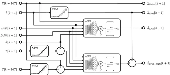
Figure 1 A schematic depicting the overall algorithm and how each method maps the inputs onto an output.

2.4. Hybrid Approach

The hybrid approach is based on a combination of CPM and ANN models. The CPM captures the physical characteristics of the building envelope by projecting the temperature to energy demand. The ANN, on the contrary, is suited to identify period demand patterns that are correlated with temporal features (such as time and day). As a result, it is expected for a hybrid approach to show advantages in forecast accuracy over the single methods. Note that the hybrid approach introduces additional implementation complexity, but the independence of the method from physical building parameters remains unchanged.

2.5. Summary of methods

A summary of the four methods incorporated in this study is shown in Figure 1. In total, seven unique inputs are used by the methods in various combinations and four different forecasts are generated. Note that the ANN and CPM boxes are duplicated for ease of visualization and boxes with the same name are identical. The hour of day (HoD) feature is used to capture the cyclic daily patterns of energy used. For that purpose, HoD is converted to a cyclical format that oscillates between 0 and 1, using:

��:;:<:[�] = � ?sin ?2 ⋅ � ⋅��[�]_{24 E , cos ?2 ⋅ � ⋅}��[�]_{24 EE}

where f is a linear combination of the two sinusoidal terms. For further explanation the reader is referred to [8]. In the next section, the output of forecasting methods are evaluated based on actual hourly demand data collected from three commercial buildings.

3. Case Study

Hourly measurements of heating and cooling loads were collected from three government office buildings located in Ottawa, Canada. Table 1 presents a summary of the buildings’ characteristics. The buildings are diverse in size, age, and energy usage intensity, which helped us better evaluate the robustness and transferability of the tested forecasting methods. The measured energy data were preprocessed to remove the noise and exclude outlier points. The resulting dataset contained reliable data recorded between spring 2016 and fall 2018 at one hour time intervals. In order to conduct an unbiased validation of the methods, datasets were split into training and testing subsets containing 80% and 20% of data, respectively.

(5)

CISBAT 2019

4

Table 1 A Summary of the characteristics of the studied buildings. Building Number of floors Floor area (m2₎ Construction year

Heating demand intensity (kWh/m2_-yr)

Cooling demand intensity (kWh/m2_-yr)

B1 4 39,000 1952 121 67

B2 13 61,000 1979 33 56

B3 21 33,000 1970 79 82

3.1. Change Point Models

For each of the three studied buildings, two CPM models are created: one for the heating season

(typically between November and April) and another for the cooling season (typically between

June and September). During the transition (or shoulder) months, either heating or cooling load

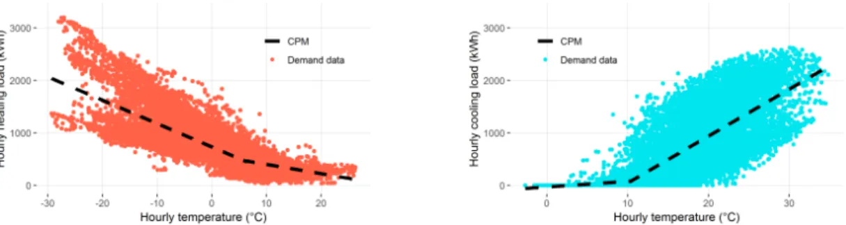
can be detected that will be added to the corresponding model. Figure 2 shows examples of

CPMs for heating and cooling seasons.

Figure 2 Examples of CPMs for the heating load of building B1 (left) and the cooling load of building B2 (right). The change point temperatures are 5 °C for heating and 10 °C for cooling.

3.2. Results

Performance of the four proposed forecasting methods were evaluated using two commonly

used metrics: the coefficient of determination (R

2

_{), and Accuracy based on the coefficient of}

variation of the root mean squared error (CVRMSE). These metrics are defined as:

�J_{= 1 −}∑ L�[�] − �"[�]M J N OPQ ∑ (�[�] − �R)N J OPQ Accuracy = 100 × (1 − ��) �� =`1�∑ L�[�] − �"[�]M J N OPQ �b

where k iterates the time steps with a maximum of N, X denotes the vector of actual demand,

�"

is the vector of forecasted demand, and

�R represents the mean of actual demand over the N

observations.

Table 2 shows the results obtained by forecasting heating and cooling loads for three buildings and three horizons of 1, 6, and 12 hours ahead. For each scenario, the best performing method(s) is highlighted. Several observations can be made by examining Table 2. First of all, it is noticed that all highlighted fields belong to either ANN or CPM-ANN methods, implying that machine learning has brought substantial benefit to our algorithm. The second observation is that the 1-hour forecasts are achieved with at least R2_{0.91 and accuracy of 92% for all scenarios. This level of accuracy is considered}

above average for hourly energy use [6]. In fact, ASHRAE Guideline 14 [9] considers a CVRMSE of 30% for hourly energy use to be acceptable, which corresponds to an accuracy of 70%.

(6)

CISBAT 2019

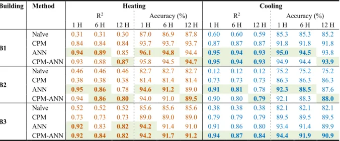
Table 2 Performance of the proposed forecasting methods for heating and cooling demands. Green shadings indicate the best performance for a given building and a forecast horizon.

Building Method Heating Cooling

R2 _{Accuracy (%)} _R2 _{Accuracy (%)} 1 H 6 H 12 H 1 H 6 H 12 H 1 H 6 H 12 H 1 H 6 H 12 H B1 Naïve 0.31 0.31 0.30 87.0 86.9 87.8 0.60 0.60 0.59 85.3 85.3 85.2 CPM 0.84 0.84 0.84 93.7 93.7 93.7 0.87 0.87 0.87 91.8 91.8 91.8 ANN 0.94 0.89 0.85 96.1 94.8 94.4 0.95 0.94 0.93 95.0 94.5 93.8 CPM-ANN 0.93 0.88 0.87 95.8 94.5 94.7 0.95 0.94 0.93 94.9 94.4 93.9 B2 Naïve 0.46 0.46 0.46 82.7 82.7 82.7 0.12 0.12 0.12 75.2 75.2 75.2 CPM 0.38 0.38 0.38 81.4 81.4 81.4 0.73 0.73 0.73 86.3 86.3 86.3 ANN 0.95 0.86 0.78 94.6 91.2 89.0 0.91 0.81 0.78 92.3 88.5 87.6 CPM-ANN 0.94 0.86 0.80 94.0 91.0 89.5 0.90 0.80 0.79 92.1 88.3 88.0 B3 Naïve 0.52 0.52 0.52 85.6 85.6 85.6 0.38 0.38 0.38 82.1 82.1 82.1 CPM 0.73 0.73 0.73 89.0 89.0 89.0 0.79 0.79 0.79 89.5 89.5 89.5 ANN 0.92 0.83 0.82 94.2 91.4 91.0 0.91 0.86 0.80 93.4 91.4 89.9 CPM-ANN 0.92 0.84 0.82 94.2 91.7 91.2 0.94 0.87 0.84 94.4 91.9 90.9

Regarding the more challenging forecast horizon of 12 hours, the CPM-ANN method shows the best performance or ties with ANN, reaching a minimum R2_{0.79 and accuracy of 88% for all scenarios. Note}

that the superiority of the CPM-ANN method for the longest forecast horizon is not tied to the performance of the CPM method for a given scenario. For example, in the case of the heating demand for building B2, the accuracy of the CPM method is even worse than the Naïve approach. However, it can still give an edge to CPM-ANN compared to ANN alone. One explanation of this behavior is that a single-layered ANN model cannot properly capture the nonlinear relation between the demand and the OAT, while the CPM can explain such a relationship even if it has a poor correlation (e.g. R2_{0.38 in the}

given example).

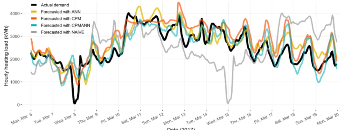
Figure 3 shows an example of 12-hour ahead forecasting of heating load for building B2, performed over two weeks in March 2017. Obviously, the Naïve approach fails to provide an accurate forecast in this case, simply because the energy consumption patterns are very different between the two weeks. A more interesting observation is how the CPM itself has a weak performance, but its output still helps the hybrid CPM-ANN approach to excel over the pure ANN model. This behaviour can be seen in two instances:

• During the weekend of March 11th_{and 12}th_{, the temperature remains almost constant, hence the}

heating demand does not show the usual day-night fluctuations. While the ANN is unable to see this abnormality and sticks to the cyclic pattern, the output from the CPM-ANN remains rather close to the actual demand.

• During the three days of March 17th_{to 19}th_{, the temperature gradually drops, but the day-night}

difference is still in place. The ANN fails to properly follow the downtrend and provides a low-accuracy forecast for the early hours on Saturday and Monday. Again, the hybrid approach takes advantage of the two underlying methods and manages to follow both the downtrend and the day-night cyclic behaviour, giving a more accurate forecast.

As a final remark, the results might suggest that the hybrid method outperforms the ANN for longer horizons. This hypothesis can be examined if the case study is expanded to longer forecast horizons, which is intended to be a part of our future work.

4. Conclusions

In this paper, we proposed and tested several methods for generating hourly forecasts of heating and cooling loads. The case study was based on hourly thermal load data collected from several office buildings located on the same campus in Ottawa, Canada, over a period of more than two years. The

(7)

CISBAT 2019

6

diversity in the parameters of studied buildings adds to the legitimacy of the obtained results. In order to avoid the problem of overtraining, the training and testing datasets were isolated.

Figure 3 Comparing actual and forecasted heating load for building B2, performed 12 hours ahead.

The results suggest that the ANN model outperforms the results obtained by the Naïve approach and by using only the CPM. However, the performance of the hybrid CPM-ANN method is superior compared to other individual models in all studied buildings, achieving a minimum accuracy of 92% for the shortest, and 88% for the longest, forecast horizon.

The outcomes indicate that ANN might fall short of modeling the nonlinear relationship between the loads and OAT as efficiently as the CPM does. The presented hybrid approach provides more accurate forecasts compared to approaches in similar studies. It also has advantages in terms of transferability, because it can be applied to a new building or portfolio of buildings without prior knowledge of physical parameters or a need for sub-metering or installing additional sensors.

For future work, we intend to test the methods for medium-term and long-term thermal demand forecasts, and will investigate whether the same conclusions still hold. Furthermore, more complex ANN models with multiple hidden layers will be deployed and compared to the current methods.

References

[1] K. Amasyali and N. M. El-Gohary, “A review of data-driven building energy consumption prediction studies,” Renew. Sustain. Energy Rev., vol. 81, pp. 1192–1205, 2018.

[2] S. F. Fux, A. Ashouri, M. J. Benz, and L. Guzzella, “EKF based self-adaptive thermal model for a passive house,” Energy Build., vol. 68, pp. 811–817, 2014.

[3] A. Dhar, T. A. Reddy, and D. E. Claridge, “A Fourier series model to predict hourly heating and cooling energy use in commercial buildings with outdoor temperature as the only weather variable,” J. Sol. energy Eng., vol. 121, no. 1, pp. 47–53, 1999.

[4] K. Yun, R. Luck, P. J. Mago, and H. Cho, “Building hourly thermal load prediction using an indexed ARX model,” Energy Build., vol. 54, pp. 225–233, 2012.

[5] S. F. Fux, M. J. Benz, A. Ashouri, and L. Guzzella, “Short-term thermal and electric load forecasting in buildings,” in CISBAT 2013, 2013, no. SEPTEMBER, pp. 495–500. [6] C. Deb, F. Zhang, J. Yang, S. E. Lee, and K. W. Shah, “A review on time series forecasting

techniques for building energy consumption,” Renew. Sustain. Energy Rev., vol. 74, pp. 902– 924, 2017.

[7] B. Gunay, W. Shen, G. Newsham, and A. Ashouri, “Detection and interpretation of anomalies in building energy use through inverse modelling,” Sci. Technol. Built Environ., vol. 25, no. 4, pp. 1–24, 2019.

[8] I. London, “Encoding cyclical continuous features,” 2016. [Online]. Available: https://ianlondon.github.io/blog/encoding-cyclical-features-24hour-time/.