CFD in support of development and optimization of the MIT LEU fuel element design

CFD in support of development and optimization of the MIT LEU

fuel element design

by

Mihai Aurelian Diaconeasa

B.Sc. Mathematics, Physics, Chemistry, University College Utrecht, 2010

SUBMITTED TO THE DEPARTMENT OF NUCLEAR SCIENCE AND ENGINEERING IN

PARTIAL FULFILLMENT OF THE REQUIREMENTS FOR THE DEGREE OF

MASTER OF SCIENCE IN NUCLEAR SCIENCE AND ENGINEERING

AT THE

MASSACHUSETTS INSTITUTE OF TECHNOLOGY

SEPTEMBER 2014

AsscCU s8rfs W4G

C 2014 Massachusetts Institute of Technology OF TECHNOLOGY All rights reserved

OCT

2

9

2014

LIBRARIES

Signature redacted

Signature of Author:

Department of Nuclear Science and Engineering

Signature redacted

August 7,2014

Certified by: .

IV

Emilio Baglietto

Assistant Professor of Nuclear Science and Engineering

Signature redacted

Thesis Supervisor

Certified by:

Lin-wen Hu Associate Director of Research Development and Utilization at the NRL

Signature redacted

Accepted by:

Mujid S. Kazimi

TE

rofessor of Nuclear Engineering

CFD in support of development and optimization of the MIT LEU fuel

element design

by

Mihai Aurelian Diaconeasa

Submitted to the Department of Nuclear Science and Engineering on August 7, 2014 in Partial Fulfillment of the Requirements for the

Degree of Master of Science in Nuclear Science and Engineering

ABSTRACT

The effect of lateral power distribution of the MITR LEU fuel design was analyzed using Computational Fluid Dynamics. Coupled conduction and convective heat transfer were modeled for uniform and non-uniform lateral power distributions. It was concluded that, due to conduction, the maximum heat flux ratio on the cladding surface is 1.16, compared to the maximum volumetric power generation ratio of 1.23. The maximum cladding temperature occurs roughly 0.5 inches from the edge of the support plate, while the peak volumetric power generation is located at the end of the fuel meat, about 0.1 inches from the edge of the support plate. Although the heat transfer coefficient is lower in the corner of the coolant channel, this has a negligible effect on the peak cladding temperature, i.e. the peak cladding temperature is related to heat flux only and a "channel average" heat transfer coefficient can be adopted. Moreover, coolant temperatures in the radial direction are reasonably uniform, which is indicative of good lateral mixing. Finally, a quasi-DNS study has been performed to analyze the effect of the fuel grooves on the local heat transfer coefficient. The quasi-DNS results bring useful insights, showing two main effects related to the existence of the grooves. First, the increased surface leads to an increase in the pressure drop and further, the flow aligned configuration of the grooves limits the ability of the near wall turbulent structures to create mixing, leading to a noticeable reduction in the local heat transfer coefficient at the base of the grooves. Overall, this leads to an effective decrease in the local heat transfer coefficient, but due to the increased heat transfer surface the global heat transfer is enhanced in comparison to the flat plate configuration. The improved understanding of the effects of grooves on the local heat transfer phenomena provides a useful contribution to future fuel design considerations. For example, the increase in pressure drop, together with the reduction in the local heat transfer coefficient indicated that the selection of a grooved wall channel instead of a smooth wall channel might not necessarily be optimal, particularly if fabrication issues are taken into account, together with the concern that grooved walls may promote oxide growth and crud formation during the life of the fuel.

Acknowledgments

I would like to express my gratitude to my supervisor, Prof. Emilio Baglietto, for the many hours spent guiding and teaching me to critically analyze my results. Also, his cluster proved pivotal in completing the second part of the thesis in a reasonable and timely manner.

Furthermore, I would also like to thank Dr. Lin-wen Hu, my other supervisor, for her availability, advice and constructive review of the thesis.

Also, I would like to acknowledge Dr. Koroush Shirvan for his assistance with running the

STAR-CCM+ code.

I deeply appreciate the support and feedback of the CFD group and, in particular, for their patience in accommodating the many nodes on the cluster that I needed to run my long simulations. It was an arduous task and their patience made it possible.

In addition, I would like to mention that this work was sponsored by the U.S. Department of Energy, National Nuclear Security Administration Office of Global Threat Reduction.

Finally, I would like to thank my wife for helping me find strength in the most critical moments and for her constant source of inspiration through endless constructive discussions.

Table of Contents

List of Figures ... 6

2. Objectives

3. Numerical Methods and Discretization Schemes ... 17

3.1 Governing Equations ... 17

3.2 Solution Algorithms...17

3.3 Discretization schemes...19

4. Turbulence Models...23

4.1 The Improved Anisotropic Turbulence Model...23

4.2 Quasi-DNS...24

5. RANS Analysis ... 25

5.1 CAD Geometry ... 25

5.2 Mesh...27

5.2.1 Volume Mesh...27

5.2.2 M odel Shakedown Testing...30

5.2.3 Near Wall Prism Layer...30

5.2.4 Grid Convergence...32

5.3 Flow features...35

5.4 Results...39

6. Quasi Direct Numerical Simulation of smooth channel flow...64

6.1 Geometry and Meshing...64

6.2 Boundary conditions ... 66

6.3 Initial conditions ... 67

6.4 Results and Validation...67

7. Quasi Direct Numerical Simulation of grooved channel flow...73

7.1 Geometry and Meshing...73

7.2 Initial and boundary conditions ... 75

7.3 Results...76

8. Comparison between Quasi-DNS results of smooth and grooved channels...81

8. Conclusions and Recommendations ... 84

9. References...85

APPENDIX A: MIT LEU Design Dimensions ... 86

APPENDIX B: Material properties ... 89

APPENDIX C: Heat transfer coefficient definition for RELAP ... 91

APPENDIX D: Vortex Test...95

List of Figures

Figure 1.1 MITR Core map showing fuel element position designations and major core structures

[2]...12

configuration...15 Figure 3.1 The SIMPLE scheme is embedded in an iterative flow solver ... 18 Figure 5.1 Isometric views of CAD model.The blue and orange colors represent the water region while the aluminum fuel plate is shown in gray ... 25 Figure 5.2 Zoomed in side section showing the grid after extrusion (the lower part from Figure

5.3)...27

28

Figure 5.4 Top view of a zoomed in section after the grid was generated where the prism layers are showed ... 28 Figure 5.5 Top view of a horizontal section zoomed in...29 Figure 5.6 Wall y+ values on the fuel element surface plotted in a perspective view...31 Figure 5.7 Water temperature profile as a function of the radial position for various grid sizes ..32 Figure 5.8 Water axial velocity profile as a function of the radial position for various grid sizes....

33

Figure 5.9 Pressure drop as a function of the base size (chosen base size encircled in black, outliers encircled in red)...34

the outlet...35

Figure 5.12 Zoomed in section around the corner inlet region of Figure 5.11 ... 36

Figure 5.13 Velocity magnitude of the coolant from the inlet to the outlet...37

Figure 5.14 Cross section in the (x,y) plane showing the tangential velocity patterns at the corn ers...3 8 Figure 5.15 Lateral power distribution in the uniform and non-uniform cases ... 39

Figure 5.16 Cladding temperatures along the axial direction...40

Figure 5.17 Temperature cross section at z=20 in ... 41

Figure 5.18 Temperature cross section at z=20 in ... 42

Figure 5.19 Radial water temperature for the line probe x...42

Figure 5.20 Three radial line probes along the y direction with 200 points ... 43

Figure 5.21 Cladding temperature along the y direction at various axial locations ... 44

Figure 5.22 Temperature along the y direction in the middle of the fuel meat at various axial locations ... 44

Figure 5.23 Temperature along the y direction in the middle of the half-coolant channel at various axial locations...45

Figure 5.24 Heat flux along the y direction at various axial locations ... 45

Figure 5.25 Heat transfer coefficient in the radial direction at at z = 20 in (Tbulk = 50.7 C)...46

Figure 5.26 Lateral cladding temperature along the axial direction ... 47

Figure 5.27 Temperature cross section at z=20 in ... 48

Figure 5.28 Temperature cross section at z=20 in ... 49

Figure 5.29 Radial water temperature for the line probe x...49

Figure 5.30 Cladding temperature along the y direction at various axial locations ... 50 Figure 5.31 Temperature along the y direction in the middle of the fuel meat at various axial

locations ... 51

Figure 5.32 Temperature along the y direction in the middle of the half-coolant channel at various axial locations...51

Figure 5.33 Heat flux along the y direction at various axial locations ... 52

Figure 5.34 Heat transfer coefficient in the radial direction at z=20 in (Tbulk = 50.7 C)...53

Figure 5.35 Temperature cross section at z = 20 in ... 54

Figure 5.36 Zoomed in temperature cross section at z = 20 in...55

Figure 5.37 Cladding temperature along the y-direction at z = 20 in...56

Figure 5.38 Heat flux along the y-direction at z = 20 in...56

Figure 5.39 Heat transfer coefficient based on the bulk temperature of the full coolant channel along the y-direction at z = 20 in (Tbulk = 50.7 C) ... 58

Figure 5.40 Local heat transfer coefficient along the y-direction at z = 20 in...58

Figure 5.41 Zoomed in cross section in the (x,y) plane from the z direction (top) ... 60

Figure 5.42 Lateral power distribution ... 61

Figure 5.43 Zoomed-in temperature cross section at z=5 in...62

Figure 5.44 Cladding temperature along the y-direction at z=5in...63

Figure 5.45 Heat flux along the y-direction at z=5in...63

Figure 6.1 Smooth channel computational domain for quasi-DNS...64

Figure 6.2 Grid used for the smooth channel quasi-DNS simulation...65

Figure 6.3 Near the wall close up of the grid used for the smooth channel quasi-DNS simulation..

66

Figure 6.7 Instantaneous non-dimensional streamwise velocity in the entire domain for smooth ch an n el...6 9

Figure 6.8 Iso-surface of Q-criterion colored with U+...70

Figure 6.9 Fully developed, channel average Nusselt number for a narrow rectangular channel [14] and the data point obtained from the quasi-DNS for smooth channel ... 72

Figure 7.1 Grooved channel computational domain for quasi-DNS ... 73

Figure 7.2 Grid used for the grooved channel quasi-DNS simulation...74

Figure 7.3 Near the groove grid used for the grooved channel quasi-DNS simulation...75

Figure 7.4 Monitor plot of the mean streamwise velocity (U) at the center of the flow domain ..76

Figure 7.5 Iso-surface of Q-criterion colored with U+...77

Figure 7.6 Instantaneous non-dimensional streamwise velocity in a plane perpendicular to the spanwise direction cutting through the middle of the groove for grooved channel...78

Figure 7.7 Mean non-dimensional streamwise velocity in a plane perpendicular to the streamwise direction for grooved channel...78

Figure 7.8 Types of walls for grooved channel -zoomed in section from Figure 7.7...79

Figure 8.1 Parallel planes from the wall...81

Figure 8.2 Parallel planes to the wall of instantaneous non-dimensional streamwise velocity contours at various y+ locations from the wall...82

Figure A-1 A schematic of MITR LEU element drawn with 18 fuel plates [9]...87

Figure A-2 A schematic of MITR LEU element drawn with 4 fuel plates [9]...88

Figure C-1 Channels in the coolant region (only the odd ones are highlighted)...91

Figure D-1 Initial setup of four vortices (Grid made of 2025 quad cells 2D)...95

Figure D-2 Results of total kinetic energy dissipation for various grids and convection term discretization schemes ... 96

List of Tables

Table 4.1 Quadratic coefficients used in the Anisotropic Turbulence Model...24

Table 5.1 Boundary conditions for the CFD model...26

Table 5.2 Meshing parameters and values...29

Table 5.3 Extrusion parameters and values for extrusion in the +z direction...30

Table 5.4 Extrusion parameters and values for extrusion in the -z direction...30

Table 5.5 Initial conditions parameters and values...30

Table 5.6 Optimization of the fuel meat width ... 60

Table 6.1 Geometry of smooth channel...65

Table 6.2 Initial flow conditions parameters and fluid properties for smooth channel ... 67

Table 6.3 Flow results for smooth channel...70

Table 6.4 Thermal results for smooth channel...71

Table 7.1 Geometry of grooved channel...73

Table 7.2 Initial flow conditions parameters and fluid properties for grooved channel...75

Table 7.3 Flow results for grooved channel...79

Table 7.4 Thermal results for grooved channel...79

Table 7.5 Thermal comparison between wall types in the grooved channel case ... 80

Table 8.1 Geometry comparison between smooth and grooved wall cases...83

Table 8.2 Flow comparison between smooth and grooved wall cases ... 83

Table 8.3 Thermal comparison between smooth and grooved wall cases ... 83

Table B-3 Temperature-dependent specific heat and density of LEU fuel meat [9]...90

Table B-4 Thermal conductivity, specific heat and density of A16061 cladding [9] ... 90

Table C-1 Coolant bulk temperature and y-location of each stripe point in Figure 45 ... 91

Table C-2 Cladding temperature for 16-stripe lateral power distribution...92

Table C-3 Heat flux for 16-stripe lateral power distribution ... 93

Table C-4 Heat transfer coefficient (HTC) for 16-stripe lateral power distribution...94

1. Introduction

In 1978 the U.S. Department of Energy (DOE) started the Reduced Enrichment for Research and Test Reactor (RERTR) Program, which targets the development of the required technology to allow the conversion of civilian facilities using high-enriched uranium (HEU - equal or more than 20% U-235) to low-enriched uranium (LEU - less than 20% U-235) fuels. Up to date, over 40 research reactors have already been converted from HEU to LEU fuels and 5 others will be converted by 2016 [1].

The MIT Reactor (MITR) is the second largest university research reactor in the US. It has been operating at 6 MW since November 2010 after the 20-year license renewal authorized by US Nuclear Regulatory Commission. It is a tank-type research reactor that is owned and operated by MIT. The MITR is composed of two concentric tanks: an outer one with heavy water (as reflector), an inner one with light water (as coolant/moderator) and a graphite reflector enclosing the heavy water tank to minimize neutron leakage. The HEU fuel used has a plate-type design cladded with grooved 6061 aluminum alloy material. Fifteen such fuel plates are assembled into a rhomboid-shaped fuel element. The reactor core has a close-packed hexagonal geometry to maximize the thermal neutron flux in the heavy water reflector region. The core region has 27 positions and is nominally loaded with twenty-four rhomboidal fuel elements and three dummy elements or in-core experiments. Six boron-impregnated stainless-steel shim blades and one cadmium regulating rod provide the reactor control (Figure 1.1). A more detailed description of the reactor design including various passive safety features can be found in the MITR Reactor Systems Manual [2]. n rod v

/

-_{- A-3} - _0-2- - flow relef hole (6)

1 \ C31 ' 4 2 3

C-4

CA B4Coolant entrance channel

C 5

/

( C-8 C-

Fxed absorber in

Fuel radial arm (3)

Element

Core

The reactor operates at atmospheric pressure with a nominal primary coolant flow rate of 2000 gpm and an average temperature of about 50 0C. The compact hexagonal core structure of about 15 inches across and with an active fuel length of about 23 inches has an average power density of about 80 kW/l. The current HEU fuel plate is designed with longitudinal grooves on the cladding to increase the heat transfer area (Figure 1.2). The unique grooved fuel plate design was adopted in 1970's during the re-design of the MITR-II. The MITR is the only research reactor in the world that uses this unique fuel design.

In the studies performed by Newton [3] on the conversion to LEU fuel at the MITR it was concluded that the conversion is possible if the high density LEU fuel becomes available. The proposed fuel with sufficient uranium density is the monolithic uranium-molybdenum (U-Mo) with molybdenum content of 10%. A new configuration, keeping the same outer fuel element geometry, but with 18 fuel plates, thinner fuel meat and cladding, was evaluated. This design may pose fabrication difficulties (i.e. meet the tolerances required), especially considering the decrease in the thickness of the fuel plate and consequently a decrease in the dimensions of the grooves.

Fuel psatepporngpaeareshwnthesheaic)[4

Fu* chmniM (I)

( FFJ1. . F~. CL

Various termal-hydali-c anayse been Nav efrel h E vrino h IR

e s til Fuel platdiesn__epe a _rstin:a_ - im n io sCL

Nea nal _Alchal reg in La s. _{_____w} et freh axia d an th et h

(~ k

Figure 1.2 Schematic of flow channel configuration of MITR (only 3 fuel plates and 1

supporting plate are shown in the schematic) edW

Various thermal-hydraulic analyses have been performed for the LEU conversion of the MITR. One of them is the study by Wang [5] in which the PLTEMP/ANL code was used. The program essentially calculates a 2-dimensional temperature solution: a 1-dimensional solution across the

fuel element at the entrance region that is repeated for each axial node along the length of the channel. In this study, two approaches were used to model the enhanced heat transfer due to the grooved fuel plates: by employing the Carnavos correlations and by using the Wong's friction

factor (obtained exclusively for the MITR [6]), and the Dittus-Boelter correlation with a 1.9 enhancement factor to account for the area of the grooves. This approach may be useful in

determining the safety margins of the reactor, however it lacks the ability to capture three-dimensional local phenomena that are important in the optimization process. Moreover, the 1.9 heat transfer augmentation factor has not been experimentally or computationally validated. As a consequence, a three-dimensional model may prove to be more suitable.

A versatile approach to model three-dimensional fluid flow and heat transfer problems is represented by computational fluid dynamics (CFD). In this work, a commercially available finite-volume (FV) based solver, STAR-CCM+, was used for accurate CFD modeling of the fuel assemblies design.

2. Objectives

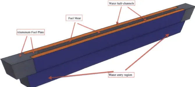
Full three-dimensional models have been developed using STAR-CCM+ for thermal-hydraulics analysis with fine axial and lateral nodalization for each fuel plate and coolant channel. As a first approximation, the geometry of the fuel plate was designed without the grooves (i.e. flat plate), in order to save computational time and because of the limited understanding of heat transfer in micro-grooves (this will be part of the next objective). The objective of this task is to model the conduction in the fuel plate and variation in the convective heat transfer rate in the axial and lateral direction of a coolant channel.

For computational efficiency, a minimal unit section has been investigated. It contains the fuel element with two water half-channels enclosing the fuel plate that contains the fuel meat (Figure 2.1). On the free sides of the water channels symmetry boundary conditions shall be imposed and an additional water region will be added under the section in order to capture the entrance effects. It should be noted that periodic boundaries would be more appropriate for the free sides, but sensitivity studies showed no measurable difference when adopting the simpler symmetric boundary.

water half-channels

Fuel MeFteIP 'ae

WVater entry region

Figure 2.1 Perspective view of the section of the modified (without grooves) flow channel configuration

The actual heating of the system is implemented as a volumetric heat source in the fuel meat region. This represents the most accurate modeling approach and allows the simulation of the correct heat transfer and temperature distributions in the meat, aluminum plate and coolant

channels.

The other objective of this project is to study and quantify the effect of the grooves. The MITR fuel element incorporates longitudinal grooves to augment heat transfer. The grooved surface

area is twice that of a flat surface. A study in 1990's by S. Parra concluded that the heat transfer enhancement factor is roughly 90% higher than that of the flat surface, however an empirical correlation predicted lower heat transfer enhancement ~ 60%. Due to the extremely small dimension of the grooves, which is comparable to the viscous sublayer thickness, it is extremely difficult to effectively quantify the heat transfer improvement. The dominant effect is expected to be an increase in the turbulence, which will lead to an increase in the heat transfer; however, its magnitude is uncertain. There is no literature that provides us with detailed quantification of this effect; therefore, a direct numerical simulation approach is the only available alternative to high accuracy experiments.

The STAR-CCM+ (v. 8.06) code was used to simulate in a quasi-DNS' fashion the effect of the

grooves. The approach in completing this task is two-fold: 1. first, perform a quasi-DNS calculation of a smooth channel flow and validate it against known databases; 2. finally, run a quasi-DNS calculation of the grooved channel flow and compare it to the smooth channel flow case.

3. Numerical Methods and Discretization Schemes

3.1 Governing Equations

The most general form of the Navier-Stokes equations for continuity and momentum in continuous integral form solved in STAR-CCM+ is given below:

a

pxdV+ p(v-

ig)di

=

SdV

(3.1)

ajpXidV+

pi®(i-,)d=-

+ pIdda+ T dd+f+f,+f,+fu

+if)dV

(3.2)

In eq. (3.1) the terms, from left to right, are the transient term, the convective flux and, respectively, the volumetric source term. In eq. (3.2), following the same direction, the following terms are present: the transient term, the convective flux, the pressure gradient term, the viscous

flux and the body force terms.

3.2 Solution Algorithms

While CFD is an extremely powerful simulation technique, its rigorous applications requires verification of the accuracy of the numerical and modeling methods. In this work, scrupulous sensitivities to all discretization, solution and modeling approaches have been performed to guarantee the quality of the simulations. The general approach of this technique is briefly discussed here.

First, the spatial solution domain is subdivided into a finite number of contiguous control volumes (CV) that can be of an arbitrary shape. STAR-CCM+ provides methods for generating different types of grids: tetrahedral, polyhedral or trimmed hexahedral. The selection of a specific type of grid depends on the specific geometrical and flow configurations and may change even from one component to another (e.g. for large aspect ratio geometries). In our models, hexahedral dominant meshes offer optimal discretization and have, therefore, been used throughout the work.

The accuracy of the finite-volume solution is strongly related to the manner in which the flow equations are discretized and solved. STAR-CCM+ employs methodologies that are based on the extensive work of Ferziger and Peric [7]. All approximations, including time and space discretization used in this work are consistently of second-order accuracy. The solution of the resulting algebraic system of equations is accomplished using a segregated iterative method based on the original SIMPLE algorithm. The linearized momentum equations are solved first, after which the pressure-correction equation is solved, and finally the temperature and turbulence quantities are solved.

STAR-CCM+ uses the semi-implicit method for the pressure-linked equations (i.e. SIMPLE

algorithm) to control the overall solution (Figure 3.1). Until convergence, for each solution update the following steps are executed:

* first, the boundary conditions are set

" the reconstruction gradients of velocity and pressure are calculated

- the velocity and pressure gradients are computed

- the discretized momentum equation is solved in order to create the intermediate velocity field

- the uncorrected mass fluxes at faces are computed

" the pressure correction equation is solved to obtain the cell values of the pressure correction and to update the pressure field (at this step the under-relaxation factor is used to add only a portion of the pressure correction to the previous iteration in order to improve the convergence)

- the boundary pressure corrections are updated

- the face mass fluxes are corrected

- finally, the cell velocities are corrected.

inner

Linear-

EquatioW-SOWo

IC-CGSTAB

AMG

onvergence?

New tIm* stp _yes

adequacy of the turbulence modeling. The extensive work of Baglietto [8] regarding turbulence modeling for fuel assembly simulations will be the starting point of obtaining an accurate representation of the flow fields, turbulent viscosities, and where the turbulent heat flux is obtained from the simple eddy diffusivity assumption.

3.3 Discretization schemes

STAR-CCM+ adopts a finite volume approach for the discretized solution of the Navier-Stokes equations. In this method the computational domain is partitioned into a finite number of control volumes that match the cells of the computational grid. Thus, eq. (3.1) and (3.2) need to be discretized and applied to each control volume in a consistent manner.

Finally, a set of linear algebraic equations is obtained with the total number of unknowns in each system of scalar equations given by the number of cells in the computational grid. It is solved with an algebraic multigrid solver (AMG).

Further, an example is given to describe the way in which the finite volume discretization methods are used in STAR-CCM+: the transport of a simple scalar quantity. The governing equation in continuous integral form is given as:

af

pqdV + po(v

-

v)da

=

oda

+ S, dV

(3.3)

V A A V

The only difference between eq. (3.1) and (3.3) is the additional diffusive flux term. By applying this transport equation to a cell-centered control volume for cell-0 the following form is derived:

d(pXOV)o+I[ po(v.5-G)],=I(roO-a) +(S Vo (3.4)

f / f

where G is the grid flux computed from the mesh motion, but can be set to zero for our interests. The transient term, the first term in eq (3.4), is used only in the unsteady (transient) calculations. The second-order temporal discretization scheme found in the implicit unsteady solver uses the solution of the current time level, n+l, together with two previous time levels, n, and n-1, in the following way:

d V0=3(pooo )n+1- 4(pooo )n+ (POOO)n

=

V

(3.5)

dt 2At

STAR-CCM+ also offers the possibility to choose a first-order temporal scheme for slow transients applications. However, in the current study, the second-order scheme is the optimal

choice for unsteady flow simulations and particularly quasi-DNS.

The convection term, the second term in eq. (3.4), is the most challenging term to discretize as it

has a tremendous effect on the accuracy and convergence of the numerical scheme. First, it is discretized in the following simple way:

[pp(*

where it is defined as the product of the scalar values and the mass flow rates at the face. The difficulty comes in when the scalar value at the face (pf) is calculated from the cell values.

Several methods are available in STAR-CCM+ among which the following need to be mentioned

and described: first-order upwind, second-order upwind, central-differencing and bounded

central-differencing.

In the first-order upwind scheme, the convective flux is defined as:

{

(rhp)

=

.(3.7)

i

rcf

01

First-order convection introduces a considerable amount of numerical dissipation that stabilizes

the solver, yet it is not desirable in simulations where discontinuities are not aligned with the grid lines. The dissipation error has the effect of smearing the discontinuities, thus decreasing the

accuracy of the solution, but this scheme is, in general, quite robust even if it is used only when

the second-order upwind scheme is not available or does not reach convergence.

When second-order accuracy is demanded, the second-order upwind scheme is required. In STAR-CCM+, it is computed in the following way:

{rnfp,,

for

20

=

rhff

where

{

1

1

are linearly interpolated from the cell values on either side of the face. Also, it was used that:

were multiplied by their limited reconstruction gradients in cells 0 and 1, respectively. The limiting of the reconstruction gradients is important in reducing the local extrema. However, although it is less dissipative than the first-order upwind scheme, it still introduces more dissipation than a central-differencing scheme.

The convective flux in the central-differencing scheme, which is also second-order accurate, is given as:

(mo) =

,i[fpo+(1-f)0

]

where

f

thus for a uniform computational grid it would have a value of 0.5.

The clear benefit of using the central-differencing scheme over the second-order upwind is seen in applications where the turbulent kinetic energy needs to be conserved. Therefore, in LES calculations, the central-differencing is more appropriate because in the upwind schemes the turbulent kinetic energy decays quite fast.

For the RANS calculations, the second-upwind scheme is still the most appropriate as the central-differencing is susceptible to dispersive error that leads to stability problems for most steady-state simulations.

The last method for discretizing the convective flux is the bounded central-differencing:

{

(rh)d

Shia

6+(1--

where at the face f, the values of the scalar quantity,

0,

fou

upwind scheme, Osou for the second-order upwind scheme and Ocd for the central-differencing

scheme. o _{is a smooth and monotone function of (the Normalized-Variable Diagram value,}

calculated based on local conditions) which satisfies the following conditions:

a(0)

and

a(;)=1 for ubf -ubf (3.14)

where Cgbf _{is called the upwind blending factor. A smaller value of (ubf ensures better accuracy,}

while a larger value increases the stability of the scheme. This method is not fully second-order accurate as the central-differencing scheme because, when the boundedness criterion is not satisfied, the scheme turns into the first-order upwind one. Thus, on coarser meshes, the bounded central differencing scheme is expected to be more dissipative than the central-differencing

scheme; however, on computational grids required by LES simulations, that should not be an issue.

In the case of complex turbulent flows, this

upwind scheme and more stable due to the

central-differencing scheme along with a

discretization the optimal choice for the DNS

c

studied grooved channel flow is expected to be.

method is more accurate than the second-order boundedness criterion. This makes the bounded

second order implicit scheme for temporal calculations of complex turbulent flows, such the

The applicability of these discretization schemes to eddy resolving methods has been verified

with a simple vortex test (Appendix D). In this test, a vortex is convected by a uniform flow on a

periodic mesh. After a convective time, given that no interactions between the various vortices

on the infinite domain are allowed, the vortex profile should be the same as the initial one. The

numerical error introduced by the discretization schemes was quantified by the L2 norm of the

difference between the initial profile and the profile after the convection. Thus, the conclusions found in the literature appropriate for our study were checked and confirmed for this version of STAR-CCM+. For more details, see the User Manual of STAR-CCM+ [10].

4. Turbulence Models

4.1 The Improved Anisotropic Turbulence Model

The Navier-Stokes equations for the instantaneous pressure and velocity fields are split into a mean and a fluctuating component in order to obtain the RANS equations. For the steady-state calculations, after time averaging, the obtained equations for the mean quantities are almost similar to the original equations, except for one more term in the momentum transport equation, the Reynolds stress tensor:

T, = -pvv' (4.1)

Therefore, the Reynolds stress tensor needs to be modeled in order to close the system of governing equations. One of the approaches widely used is the eddy viscosity models, with the assumption that the Reynolds stress tensor is proportional to the mean strain rate:

T = 2p1,S (4.2)

It introduces the concept of turbulent viscosity (pt) that is derived from some additional scalar quantities, each transported by their own equation. For example, in the case of the K-Epsilon turbulence model, two transport equations are solved for the turbulent kinetic energy (k) and its dissipation rate (E).

Accurate flow and temperature predictions require the use of adequate turbulence modeling, which still remains the most challenging component of the CFD application. In particular, the often overlooked turbulence anisotropy can have very noticeable effects on fuel assembly flow and heat transfer behavior. Among the possible effects of the anisotropy of the Reynolds stresses, one that is more evident is the formation of turbulence driven secondary flows in non-circular ducts. These secondary motions, also known as secondary flow of Prandtl second kind, although of small magnitude, highly contribute to the turbulence redistribution inside the sub-channels where the transport in the circumferential direction related to the secondary vortex is of the same order of magnitude of the turbulent transport.

In order to accurately predict turbulence in the fuel geometry, the Improved Anisotropic Turbulence Model was used [8]. Thus, instead of the customary eddy-viscosity assumption, a quadratic stress-strain relation is employed (4.3):

puuj =

-pk8..

SySkSkl

where the formulation of the coefficients multiplying the quadratic terms respects the realizability conditions:

Cl = CNL1 (cNL4 +CNL5s )C(

U

CNL3 (45)

(CNL4 + CNL5S )C

C2 = CNL2 (4.6)

(CNL4 + CNL5 3

and the adopted coefficients CNLJ, CNL2, CNL3., CNL4, CNL5 are given in Table 5.

Table 4.1 Quadratic coefficients used in the Anisotropic Turbulence Model

4.2 Quasi-DNS

The accuracy of the DNS studies lies in the fact that the Navier-Stokes equations are numerically solved without any modeling; therefore, no turbulence model is required. In fact, DNS simulations are often used to validate the turbulence models. With this simulation technique all the length scales of turbulence are resolved: from the integral length scale, associated with the geometrical features of the boundaries, up to the smallest dissipative scales (i.e. Kolmogorov length scales). Thus, defining a sufficiently fine mesh is vital in order to obtain an accurately resolved solution.

Another aspect of a DNS analysis is related to the selection of the numerical schemes. In general, the DNS studies are performed with fourth order numerical schemes in order to reduce the numerical errors. Nonetheless, in this study, second order schemes were used for both spacial and temporal discretizations. As a consequence, it is important to note here that this approach to doing DNS calculations is reasonable; however, its accuracy is not fully verifiable as the DNS standards would normally require. Thus, this variation of the DNS method is referred to as quasi-DNS [11]. Coefficient Value CNLI

0.8

11

1000

5.

RANS Analysis

5.1 CAD Geometry

The CAD geometry from Figure 2.1 was built using the 3D-CAD parametric solid modeler of the STAR-CCM+ package. The three geometrical projections (front, top and side) are given below in Figure 5.1. The geometry is based on the MIT LEU design (Appendix A). All the dimensions were taken from the MITR Reactor Systems Manual [2], except for the height of the column (that is, the flow or z direction). This is because, in order to achieve an optimal mesh distribution, the outlet sections of the three materials (i.e. aluminum, water, UO2) were extruded. A number of

150 layers with a stretching factor of 1.75 was used. Moreover, the boundary interface conditions

implemented are given in Table 5.1.

Front

I

Top

Side

Figure 5.1 Isometric views of CAD model.The blue and orange colors represent the water region while the aluminum fuel plate is shown in gray

25

Table 5.1 Boundary conditions for the CFD model

Surface Region Boundary Thermal Shear Stress

Specification Specification

Fuel Meat Wall Conjugate heat

-transfer (volumetric heat source)

Aluminum Plate Wall Adiabatic

-Water Inlet Velocity -

-Water Sides Symmetry Plane -

-Water/Aluminum Plate Wall Adiabatic No-Slip

interface

Water Outlet Pressure Outlet -

-The main difference between this CAD model and the MIT LEU design (Appendix A) is that the grooves with a depth of 10 mils featured on the cladding surface were removed. Also, the cladding width was increased by 5 mils on each side such that the effective interior channel thickness is preserved (see Figure 5.5 _{for a zoomed in section showing the absence of the} grooves).

5.2

Mesh

5.2.1 Volume Mesh

The user driven, automatic meshing tools in STAR-CCM+ have been used to generate the optimal geometrical discretization. For this design, the trimmed cell mesher and the prism layer mesher were used. The latter is used only in the water regions to create the necessary orthogonal prismatic cells near the wall boundaries in order to improve the accuracy of the flow solution in the boundary layer region. For the rest of the regions, the former method produced a predominantly hexahedral mesh with minimal cell skewness and adequate local refinement for accurately modeling the various local features. The parameters and values used in generating the mesh are given in Table 5.2. Moreover, as it was mentioned in the previous section, the outlet sections of the three materials (i.e. aluminum, water, U02) and the inlet section of the entry water

channel were extruded from the inlet and outlet plane mesh surface. The details are given in Table 5.3 and Table 5.4 and a side section is given in Figure 5.2 to show the results, while Figure

5.3 offers a better perspective of where the section from Figure 5.2 is positioned. The thickness

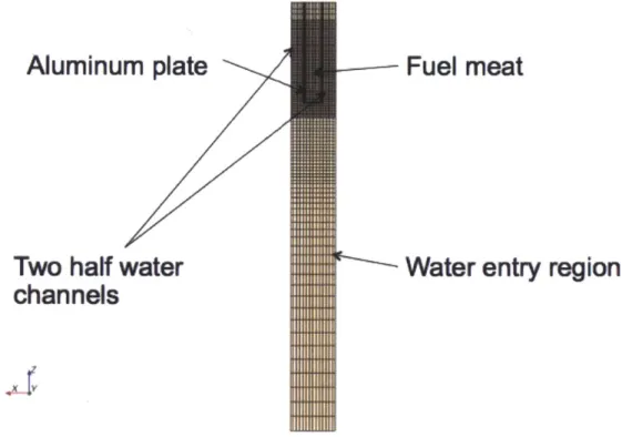
of the near-wall prism layer, the total prism layer thickness and the number of prism layers were obtained iteratively by analyzing the wall y+ (see definition in Eq. 6.3) values obtained from running the simulation (further details given in section 5.2.3). The fine grid obtained can be seen in Figure 5.4 where a zoomed-in section is plotted (close to the corner of the fuel meat). Finally, in Figure 5.5 a top view horizontal section is given for more insight.

Aluminum plate

Fuel meat

Two half water

_{Water entry region}

channels

Figure 5.2 Zoomed in side section showing the grid after extrusion (the lower part from Figure 5.3)

Outlet

Inlet

Figure 5.3 Front view of the full geometry after the grid was

1%)

Wate-channel

I

-generated (transparency set to

Aluminum

plate

Fuelms

Figure 5.4 Top view of a zoomed in section layers are showed

after the grid was generated where the prism

+

IV

Of

! a E

Figure 5.5 Top view of a horizontal section zoomed in Table 5.2 Meshing parameters and values

29

Parameter Value

Base Size 0.005 in (0.127 mm)

Maximum Cell Size (Relative to Base) 200%

Number of Prism Layers 6

Prism Layer Thickness 0.006 in (0.1524 mm)

Thickness of Near Wall Prism Layer 0.0001 in (0.00254 mm)

Surface Growth Rate 1.5

Template Growth Rate Fast

Custom Boundary Growth Rate 8

F=

r

r"

7Tf

Table 5.3 _{Extrusion parameters and values for extrusion in the +z direction}

Parameter Value

Extrusion Type Hyperbolic tangent

Number of Layers 150

Stretching 1.75

U

Table 5.4 Extrusion parameters and values for extrusion in the -z direction

Parameter Value

Extrusion Type Hyperbolic tangent

Number of Layers 25

Stretching 1.25

5.2.2 Model Shakedown Testing

In order to test the model performance, verify any potential issue with grid quality, optimize the grid, particularly in the near wall regions, and perform the necessary sensitivity studies, a first set of runs were performed with a uniform heat flux as a first approximation. The data are given in Table 5.5. The material properties used are given in Appendix B.

Table 5.5 Initial conditions parameters and values

5.2.3 Near Wall Prism Layer

Given the challenging low Reynolds number flow conditions of this application (i.e. laminar and transition flow), and the importance of accurate hear transfer coefficient prediction, the use of wall functions was discarded in favor of a more rigorous near wall modeling. The transport

Parameter Value

Inlet Velocity 3 m/s

Inlet Temperature 40 C

Turbulent Intensity 20%

Turbulent Length Scale 0.2525 in (6.4135 mm)

Turbulent Velocity Scale 1 m/s

equations are solved all the way to the wall in what is usually referred to as a low y+ approach or wall resolved method. Therefore, in order to accurately resolve the viscous sublayer, a fine grid had to be generated. Accordingly, the thickness of the near the wall prism layer, the total prism layer thickness and the number of prism layers were evaluated. Finally, as shown in Table 5.2, 6 prism layers were used to resolve the y+ 40 region (the edge of the viscous sublayer) and the y+ was kept below 0.5 at the first cell near the wall (Figure 5.6). This approach allows further applicability of this computational mesh to laminar and transitional cases.

00 0.", WON Y+ 04W

~-~- J

0 80

Figure 5.6 Wall y+ values on the fuel element surface plotted in a perspective view

5.2.4 Grid Convergence A grid sensitivity study is

simulation speed while discretization error. Various

required in order to evaluate the cell base size that optimizes the minimizing computational usage, and more importantly, the parameters are analyzed to check the grid convergence.

First, the water temperature profiles as a function of the radial position for various base sizes from 0.003 to 0.0075 in were plotted along a line probe normal to the wall at a height of 12 in (fully developed region, see Figure 5.10 for the line probe position). From the plot (Figure 5.7), it can be observed how fine grid sizes (between 0.003 and 0.005 in) produce very similar results, which is indicated by the almost perfect overlap of the profiles. However, it is interesting to note that as the base size is increased to 0.007 in and 0.0075 in different values are obtained. This sudden change is a good demonstration of the modeling challenges related to the low Reynolds number and the need for grid evaluation.

As a further confirmation, using the same line probe, the axial velocity was plotted against the radial position for the same base sizes as above (Figure 5.8). Again, the profiles for the base sizes between 0.003 and 0.005 are in excellent agreement, while the higher base sizes show lower velocity profiles.

Temperature (C) profile along the normal at z =12"

for various base sizes (mil

42 A A A A A 40 3. A A A " A A A A A A A A 36 5U "Mg 0 U U 0000 0005 0010 0015 0020 Positoo, Iin) 0075 0030 0035 0.040

temperature profile as a function of the radial position for various grid AA Us 4 7= If 10 Figure 5.7 Water sizes

Velocity[k] (m/s) profile along the normal at z=12" for various base sizes (mil

a41P _{9 v V}

I9

_I9

9P

"

9

Figure 5.8 Water axial velocity

sizes

p.

profile as a function of the radial position for various grid

Based on the results, the base size of 0.005 in was chosen as it provides optimal computational economy while producing highly accurate predictions. One final check was performed by looking at the pressure drop for the same base sizes from 0.003 to 0.0075 in (encircled in red) as shown in Figure 5.9. While the pressure drop shows smaller sensitivity to the grid quality, the same two outliers for base sizes 0.007 in and 0.0075 in are found.

33

a-CD w a-2.a4UOEt04 2 SAOr.E+04 2.E800C E+C04 2.940e E+#04 2 6200OE+04 2.&ODOC.04 2.7806E+04 2.7 50( "04 0 rp?c

Figure 5.9 Pressure drop outliers encircled in red)

Uc

0

as a function of the base size (chosen base size encircled in black,

-p+9

r'dbe

--A

~Y/

5.3 Flow features

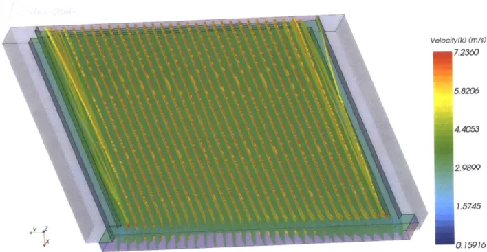
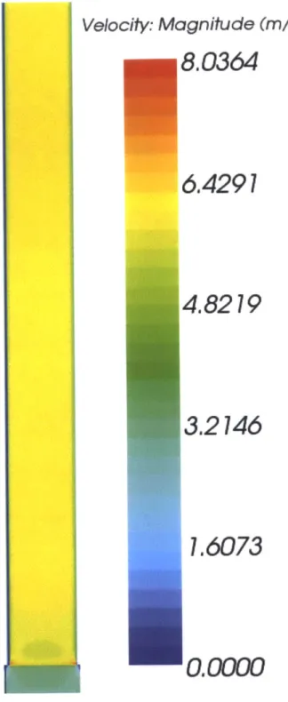
Although the inlet velocity is 3 m/s at the entrance channel, because the flow is split into two half-channels (see Figure 5.11 for streamlines that follow individual seed points from the inlet to the outlet, or even better, in a zoomed in section Figure 5.12) the streamwise velocity approximately doubles. In order to see this, the velocity magnitude was plotted by showing one side of the coolant channel (Figure 5.13).

Velocity(k) (m/s)

I7.2360

U0.15916

Figure 5.11 Perspective view of streamlines of the velocity along the z direction from the

inlet to the outlet

1:1

Velocity: Magnitude (m/s)

8.0364

6.4291

4.8219

3.2146

1.6073

O.0000

Figure 5.13 Velocity magnitude of the coolant from the inlet to the outlet

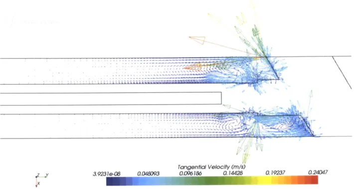
In Figure 5.11 and Figure 5.12 it can be seen that, on the edges of the lateral direction (y), the streamlines do not follow a straight direction parallel to the z direction, but they shift in various directions. This is because the improved anisotropic turbulence model used is able to capture the secondary recirculation flows (Figure 5.14). Given that the maximum magnitude of the

tangential velocity is about 8% of the inlet velocity, it was confirmed that the secondary flows need to be included for the accurate prediction of the flow and temperature distributions.

T 1

ti4«

3.9231e-08 0.048093

Tangential Velocity (m/s)

0096186 0.14428

Figure 5.14 Cross section in the (x,y) plane showing the tangential velocity patterns at the

corners .z it

yX

0.19237

5.4

Results

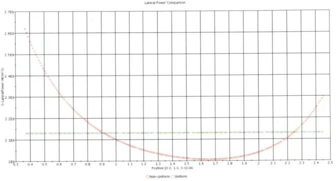
Finally, the boundaries representing the operating power were implemented. The volumetric power generation was implemented both as uniform and non-uniform in the lateral direction, as is shown in Figure 5.15. In order to have the consistent results, the uniform lateral power was obtained from the given non-uniform lateral power distribution by keeping the area under the curves constant.

For further guidance in the results section, is important to note that the width of the fuel meat has

a length of 2.082 in (from 0.36926 in to

2.451226

in on the y-axis).

Lateral Power Comparison

2. 7E9 6E9 __ SE9 __ __ 4E9 ___ 3E9---2E9 - - - -___ 2E0.3 04 05 06 0.7 0.8 0.9 1 11 1.2 1.3 1.4 1.5 1.6 17 1.8 1.9 2 21 22 23 24 2. Position [0.0. 1.0, 0.0 Oin) )Non-Uniform Uniform

Figure 5.15 Lateral power distribution in the uniform and non-uniform cases 5.4.1 Uniform Volumetric Power Generation

The uniform power generation case results are given first. In what follows, the various temperature profiles are checked.

The cladding temperature along the axial direction is plotted in order to check the convergence of the simulation up to the outlet (Figure 5.16). It can be seen that the cladding temperature profile in the lateral direction is the same along the full length of the channel.

39

}

Temperature (C)

69.235

63.388

57.541

51.694

45.847

40."x

i

I

In order to see the heating patterns in all the materials, a cross section was cut radially at a height of 20 in (Figure 5.17). As it can be seen, the fuel meat has a peak temperature of 73 C, the aluminum plate has a temperature of about 50 C on the sides, and the water temperature is about

51 *C in the middle of the channel and about 44 0C at the corners.

9mperoture (C)

73.56

67.68

T

Figure 5.17 Temperature cross section at z=20 in

61.80

55.93

50.05

44.17

At a height of 20 in, a zoomed in view of the same horizontal cross section is shown in Figure

5.18.

Temperature (C)

73.56

67.68

61.80

55.93

50.05

44.17

Figure 5.18 Temperature cross section at z=20 in

The water temperature in the radial direction of the line probe x at a height of 20 in (similar to the line probe from Figure 5.10) is plotted in Figure 5.19. It should be noted that the middle of

the water channel is located at position 0.

0-Radial Temperature 67 65 64 63 61 .60 g57 56 55 54 53 52 50 0.01 0.02 Position [1.0, 0.0, 0.0 (in) a 0.03 0 04 0.05 VY - , 0

A set of radial line probes along the y direction (horizontal) were created at various axial locations: 5, 10 and 20 in. One was cut through the middle of the coolant half-channel, one along the cladding and the other one through the middle of the fuel meat (Figure 5.20).

.Z ,y

Figure 5.20 Three radial line probes along the y direction with 200 points

The cladding temperature profiles along the y direction are given in Figure 5.21, the temperature profiles along y cutting through the middle of the fuel meat are given in Figure 5.22, while the temperature profiles through the middle of the coolant half-channel are plotted in Figure 5.23. It can be noted that the temperature values on the sides in the y direction are not symmetrical due to the anti-symmetric geometry. Moreover, a gradual increase in the temperature profiles as the

height increases can be observed in both figures.

Next, the heat flux at the cladding along the lateral direction is plotted at various axial locations

(Figure 5.24).

43

0-Cladding Temperature along yp 69 67 03 057 53 51 49 47 45 ---.... _ 43 o 1 2 Poston [00, 1.0, 0.0111In)

'Cupyr l~ne-poboe-alonov at--to-.r Copy ofline-pobe-aln--a-z~-?n-Iri CopvoTlile-probe--along0-v-at-z- "-i

Figure 5.21 Cladding temperature along the y direction at various axial locations

Pd

a

Temperature along v -middle of the fuel meat

73r_

~....

Copyof Copyof line-probe-along-y-at-z-10-in Copvoi Copy of line-probe-along-y-at-z-S-In Copvof Copvof line-probe-along-y-at-z-20-in

Figure 5.22 Temperature along the y direction in the middle of the fuel meat at various

0-Coolam Temperature along y 52 50 49

~48

Figure 5.23 Temperature along the y direction in the middle of the half-coolant channel at

various axial locations

0-Heat Flux along v

G00000 400000 400000 200000 , 100000 Position 10 0, 1.0, 0.01 (in)

Copyof line-probe-along-y-at-z-10-in OCopyof line-probe-along-y-at-z-20-in Copy of line-prole-along-y-at-z-5-in

Figure 5.24 Heat flux along the y direction at various axial locations

Since the flow is already fully developed at z = 5 in (see Figure 5.16), the does not change as the height is increased.

Finally, the heat transfer coefficient based is plotted along the y direction (following cladding) at z = 20 in (Figure 5.25).

on the bulk coolant temperature the line probe from Figure 5.20

heat flux distribution

of the whole channel restricted only to the

01-HTC along y 49000 48000 47000 46000 ___ 45000___ ______ ______ 44000 ______ a43000 __ 942000 41000___ 40000 __ c3000 __ 37000 36000 04 05 06 07 08 09 1 1.1 1.2 13 1.4 1.5 1.6 1.7 1.8 1.9 2 2.1 2.2 20 2.4 2.' Position 10.0, 1.0, 0.01 (in) .HTC Copy of line-probe-along-y-at-z-20-in

Figure 5.25 Heat transfer coefficient in the radial direction at at z = 20 in (Tbulk = 50.7 *C)

5.4.2 Non-Uniform Lateral Power Distribution

Again, the lateral cladding temperature patterns along the axial direction are plotted in order to check the convergence of the simulation up to the outlet for the non-uniform lateral power distribution case (Figure 5.26). _{As in the uniform case, it can be seen that the cladding}

temperature profile in the lateral direction is the same along the full length of the channel.

_I

7-NI\

Temperature (C)

1.069

64.855

58.641

52.428

46.214

40.0

Figure 5.26 Lateral cladding temperature along the axial direction

47

In order to see the heating patterns in all the materials, a cross section was cut radially at a height of 20 in (Figure 5.27). The fuel meat has a peak temperature of 75 C, the aluminum plate has a temperature of about 50 *C on the sides, and the water temperature is about 51 0C in the middle of the channel and about 44 *C at the corners.

Temperatu 1 ₇₅

69

50

FU

044

Figure 5.27 Temperature cross section at z=20 in

re (C)

.86

.60

.34

.08

.82

.56

Temperature (C)

75.86

69.60

63.34

57.08

50.82

44.56

Figure 5.28 Temperature cross section at z=20 in

The water temperature in the radial direction of the line probe x at a height of 20 in (similar to

the line probe from Figure 5.10) is plotted in Figure 5.29. The middle of the water channel is

located at position 0.

Figure 5.29 Radial water temperature for the line probe x

A set of radial line probes along the y direction (horizontal) was done at various axial locations (i.e. 5, 10 and 20 in) in the same way as in the uniform case from Figure 5.20.

The cladding temperature profiles along y are given in Figure 5.30, the temperature profiles along y cutting through the middle of the fuel meat are given in Figure 5.31, while the temperature profiles through the middle of the coolant half-channel are plotted in Figure 5.32. It can be noted that the temperature values on the sides in the y direction are not symmetrical due to the anti-symmetric geometry. Moreover, a gradual increase in the temperature profiles as the height increases can be observed in both figures.

0-Cladding Temperature along y 71 70 69 ' 65 63 -- _______ 1 ., -,--( A57 E 53 51 47 45 43 1 2 3 Position [0.0, 1.0, 0.0[ (In)

Copyofline-probe-along-y-at-z-10-in Copyofline-probe-along-y-at-z-20-in Copyofline-probe-along-y-at-z-5-in

Temperature along y - middle of the fuel meat

80

70

50

0 1 2

Copv of Copy of line-probe-along-v-at-z-5-ii

Position [0.0. 1.0, 0.01 (I

Copvof Cop'%,of lwe~-probe-along-v- ail-z-20-r. lopy of Copy of line-prone-along-yat-z-1-n

Figure 5.31 Temperature along the y direction in the middle of the fuel meat at various

axial locations

0-Coolan Temperature along y 52 51 50 49 40 -'47 0 43 41 40 o0oh 40 1 2 3 Position [0.0, 1 0, 0.0] (in)

Oline-probe-along-y-at-z-10-in llne-probe-along-v-at-z-20-in Qline-probe-along-v-at-z-5-in

Figure 5.32 Temperature along the y direction in the middle of the half-coolant channel at

various axial locations