HAL Id: hal-00316946
https://hal.archives-ouvertes.fr/hal-00316946
Submitted on 1 Jan 2001
HAL is a multi-disciplinary open access
archive for the deposit and dissemination of
sci-entific research documents, whether they are
pub-lished or not. The documents may come from
teaching and research institutions in France or
abroad, or from public or private research centers.
L’archive ouverte pluridisciplinaire HAL, est
destinée au dépôt et à la diffusion de documents
scientifiques de niveau recherche, publiés ou non,
émanant des établissements d’enseignement et de
recherche français ou étrangers, des laboratoires
publics ou privés.
the high-latitude magnetopause by the Cluster
spacecraft and pulsed radar signatures in the conjugate
ionosphere by the CUTLASS and EISCAT radars
J. A. Wild, S. W. H. Cowley, J. A. Davies, H. Khan, M. Lester, S. E. Milan,
G. Provan, T. K. Yeoman, A. Balogh, M. W. Dunlop, et al.
To cite this version:
J. A. Wild, S. W. H. Cowley, J. A. Davies, H. Khan, M. Lester, et al.. First simultaneous observations
of flux transfer events at the high-latitude magnetopause by the Cluster spacecraft and pulsed radar
signatures in the conjugate ionosphere by the CUTLASS and EISCAT radars. Annales Geophysicae,
European Geosciences Union, 2001, 19 (10/12), pp.1491-1508. �hal-00316946�
Annales
Geophysicae
First simultaneous observations of flux transfer events at the
high-latitude magnetopause by the Cluster spacecraft and pulsed
radar signatures in the conjugate ionosphere by the CUTLASS and
EISCAT radars
J. A. Wild1, S. W. H. Cowley1, J. A. Davies1, H. Khan1, M. Lester1, S. E. Milan1, G. Provan1, T. K. Yeoman1, A. Balogh2, M. W. Dunlop2, K.-H. Fornacon3, and E. Georgescu4
1Department of Physics & Astronomy, University of Leicester, Leicester LE1 7RH, UK
2Space and Atmospheric Physics, Blackett Laboratory, Imperial College, London SW7 2BZ, UK 3Technische Universit¨at Braunschweig, Mendelssohnstraße 3, 38106 Braunschweig, Germany 4Max-Planck-Institut f¨ur Extraterrestrische Physik, PO Box 1312, 85741 Garching, Germany
Received: 16 March 2001 – Revised: 20 June 2001 – Accepted: 16 July 2001
Abstract. Cluster magnetic field data are studied during an
outbound pass through the post-noon high-latitude magne-topause region on 14 February 2001. The onset of several minute perturbations in the magnetospheric field was ob-served in conjunction with a southward turn of the interplan-etary magnetic field observed upstream by the ACE space-craft and lagged to the subsolar magnetopause. These per-turbations culminated in the observation of four clear netospheric flux transfer events (FTEs) adjacent to the mag-netopause, together with a highly-structured magnetopause boundary layer containing related field features. Further-more, clear FTEs were observed later in the magnetosheath. The magnetospheric FTEs were of essentially the same form as the original “flux erosion events” observed in HEOS-2 data at a similar location and under similar interplanetary conditions by Haerendel et al. (1978). We show that the na-ture of the magnetic perturbations in these events is con-sistent with the formation of open flux tubes connected to the northern polar ionosphere via pulsed reconnection in the dusk sector magnetopause. The magnetic footprint of the Cluster spacecraft during the boundary passage is shown to map centrally within the fields-of-view of the CUTLASS Su-perDARN radars, and to pass across the field-aligned beam of the EISCAT Svalbard radar (ESR) system. It is shown that both the ionospheric flow and the backscatter power in the CUTLASS data pulse are in synchrony with the mag-netospheric FTEs and boundary layer structures at the lat-itude of the Cluster footprint. These flow and power fea-tures are subsequently found to propagate poleward, form-ing classic “pulsed ionospheric flow” and “poleward-movform-ing radar auroral form” structures at higher latitudes. The com-bined Cluster-CUTLASS observations thus represent a di-rect demonstration of the coupling of momentum and energy
Correspondence to: J. A. Wild ([email protected])
into the magnetosphere-ionosphere system via pulsed mag-netopause reconnection. The ESR observations also reveal the nature of the structured and variable polar ionosphere produced by the structured and time-varying precipitation and flow.
Key words. Ionosphere (auroral ionosphere)
Magentosphe-ric physics (magnetopause, cusp and boundary layers; mag-netosphere-ionosphere interactions)
1 Introduction
Reconnection at the dayside magnetopause boundary is the dominant mechanism by which energy and momentum are transferred from the solar wind into the Earth’s magneto-sphere. As such, an understanding of reconnection at this boundary and its consequences is central to any efforts to quantify the solar wind-magnetosphere coupling. Signatures indicating that the reconnection process is often of a transient nature were first obtained by Haerendel et al. (1978) using high-latitude magnetic field data from the HEOS-2 space-craft, and by Russell and Elphic (1978, 1979) using lower latitude data from ISEE-1 and -2. These studies revealed the existence of characteristic transient signatures in the mag-netic field in the vicinity of the magnetopause, which have a time scale of a few minutes, and a recurrence interval of ∼5–10 min. These signatures were termed “flux erosion events” by Haerendel et al. (1978) and “flux transfer events” (FTEs) by Russell and Elphic (1978, 1979). Later, Rijnbeek and Cowley (1984) demonstrated that these represent essen-tially the same phenomenon. The characteristics of these events include bipolar signatures in the field component nor-mal to the magnetopause, field tilting effects in the plane of the magnetopause, and mixed plasma populations
origi-nating both in the magnetosphere and magnetosheath (e.g. Paschmann et al., 1982; Farrugia et al., 1988).
Russell and Elphic (1978, 1979) offered a physical inter-pretation of FTEs as arising from transient (a few minutes) and spatially localised (few RE) episodes of reconnection at
the magnetopause. The reconnection interpretation was later supported by studies showing a strong association of FTE occurrence with southward fields in the magnetosheath and interplanetary medium (Rijnbeek et al., 1984; Berchem and Russell, 1984; Kawano and Russell, 1997). Southwood et al. (1988) and Scholer (1988) suggested that the structures could also be formed by transient reconnection at sites that are more extended along the magnetopause. Most recently, Milan et al. (2000) have presented evidence based on UV auroral imager data and HF radar data suggesting that the re-connection site may at any one time be spatially localised, but that it propagates wave-like over the magnetopause for extended distances and intervals of time (at least ∼ 10 min).
The spatial structure of the reconnection geometry at the magnetopause has an impact on the form of the expected flow signatures in the dayside ionosphere, depending upon whether it is patchy, extended, or wave-like, and a vari-ety of theoretical pictures have been put forth to describe the expectations in these cases (e.g. Southwood, 1985, 1987; Cowley, 1986; McHenry and Clauer, 1987; Lockwood et al., 1990; Wei and Lee, 1990; Cowley et al., 1991; Cowley and Lockwood, 1992; Milan et al., 2000). Correspondingly, considerable efforts have been made to observe the signa-tures of FTEs in the polar ionosphere. The first ground-based observations which were identified as potential flux transfer events were published by van Eyken et al. (1984) and Goertz et al. (1985). Van Eyken et al. (1984) studied EISCAT UHF radar data and observed a brief northward ex-cursion in an otherwise westward flow. Goertz et al. (1985) used data from the STARE VHF coherent radar to detect a convection boundary in the radar’s field-of-view. Poleward of this boundary, the flow was observed to be anti-sunward, with an occasional significant north-south component. Flows across the convection boundary occurred sporadically in spa-tially localised regions with scale sizes between 50–300 km, and with a repetition rate of the order of minutes. In one particular event, Goertz et al. (1985) reported observing a poleward-moving transient which grew and decayed over a 4 min interval. The transient flows were interpreted as the result of newly-reconnected flux tubes being pulled pole-ward by the magnetosheath flow. Subsequently, Lockwood et al. (1989, 1993) used data from the EISCAT incoherent scatter radar to observe flow enhancements which were as-sociated with dayside auroral transients. These were also interpreted as being related to FTEs observed at the mag-netopause.
HF coherent radars have more recently provided a wealth of observations which have similarly been associated with flux transfer events. The radars typically observe high veloc-ity anti-sunward transient flow in the cusp ionosphere. Such signatures were first assumed to be the response to transient magnetopause reconnection by Pinnock et al. (1993, 1995)
and Rodger and Pinnock (1997). Quasi-periodic sequences of such events, termed pulsed ionospheric flows (PIFs), have subsequently been examined both statistically and individ-ually, and the spatial extent of these events, their flow ori-entation, MLT occurrence, dependence on IMF oriori-entation, and repetition frequencies have been extensively examined (Provan et al., 1998, 1999; Provan and Yeoman, 1999; Milan et al., 1999b, 2000; McWilliams et al., 2000).
In spite of the progress made in characterizing FTEs at the magnetopause and their effects in the polar ionosphere, it was not until the study of Elphic et al. (1990) that simultane-ous observations of an FTE at the magnetopause and the flow response in the near-conjugate ionosphere became available. Although the EISCAT radar observations were limited to two pointing directions and a 5 min measurement cycle, Elphic and co-workers showed evidence of transient reconnection at the magnetopause and a simultaneous flow response in the polar ionosphere. These data, obtained during one observing interval, remained unique until the advent of the Equator-S mission. Neudegg et al. (1999) presented a single case study of a southward turning of the IMF which resulted in the observation of a clear magnetospheric FTE in the magne-tometer data of the Equator-S spacecraft, located in the vicin-ity of the magnetopause. This was accompanied almost si-multaneously by the onset of transient poleward-propagating flow signatures in the SuperDARN Hankasalmi (CUTLASS) radar. Prior to the southward turning of the IMF, there had been an extended interval of northward IMF during which no such ionospheric signatures were observed. The iono-spheric flow data in this study was of excellent quality, with a 30 km range resolution, and a 2 s dwell time per beam, giv-ing a full scan of the 16 radar beams every 32 s, allowgiv-ing for an accurate picture of the ionospheric convection to be deduced. This ionospheric flow response was fully in ac-cord with those HF radar results based upon ground-based data alone. Subsequently, it was demonstrated by Neudegg et al. (2001) that the high-latitude convection response to the reconnection process associated with this magnetopause FTE excited strong UV aurora equatorward of the footprint of the newly-reconnected field lines.
A more statistical study was performed by Neudegg et al. (2000), who examined the characteristic signatures of FTEs at the magnetopause, as observed by the Equator-S spacecraft, with the characteristic pulsed anti-sunward flows observed in the HF radar data in the ionosphere at the con-jugate footprint of Equator-S. They found a strong associa-tion between the magnetopause and ionospheric phenomena. They also suggested that for FTEs with a repetition rate of greater than 5 min, a clear one-to-one correlation often ex-isted between magnetopause and ionospheric events. For faster repetition rates, the ionospheric response began to re-semble that expected from a continuous flow excitation. The overall flow patterns observed in association with the FTEs were in broad agreement with those predicted theoretically, but showed a wide spectrum of responses on an event-by-event basis.
Figure 1
Fig. 1. Plots showing the outbound orbit of the Cluster 1 (Rumba) spacecraft projected onto the GSM X − Z (left) and X − Y planes (right) on 14 February 2001. The position of the spacecraft at one-hour intervals of UT is indicated by the purple circles, for 06:00–16:00 UT. The interval of principal interest here is ∼ 09:00–11:00 UT, adjacent to the magnetopause. The locations of the other Cluster spacecraft are indicated by additional coloured circles, as indicated by the key, where the separation from Cluster 1 has been magnified by a factor of ten in order to more clearly indicate the form of the tetrahedral configuration. Tsyganenko-96 model field lines (short-dashed lines) are drawn at hourly intervals through the position of Cluster 1. This field model is parameterised by the solar wind dynamic pressure p, the IMF, and Dst.
The values chosen here are p = 1 nPa, IMF BY =3 nT, IMF BZ= −5 nT, and Dst = −15 nT, corresponding to prevailing conditions near
the time of the boundary region encounter (∼ 10:00–11:00 UT). The field lines are terminated when they reach the model magnetopause. The model magnetopause position in the plane of the two diagrams is shown by the solid lines. In the right-hand panel, field lines are also terminated when they reach the GSM equatorial plane.
Neudegg et al. the number of ground-satellite conjunctions available for investigation remain few in number, and our knowledge of the detailed ionospheric flow response to vari-ous magnetopause reconnection scenarios, for example, FTE size, location, propagation, and repetition rates, remains incomplete. For this reason, an extensive programme of ground-based radar observations is currently under way to observe ionospheric conditions in the regions conjugate to the Cluster spacecraft, particularly during spacecraft traver-sals of the magnetopause region. In this paper, we present the first simultaneous observations of FTEs in the magne-topause region by the Cluster spacecraft, and pulsed features in the conjugate ionosphere by the CUTLASS and EISCAT Svalbard radars.
2 Instrumentation
This paper investigates magnetometer data from an outbound pass of the Cluster spacecraft through the post-noon high-latitude magnetopause region, together with simultaneous ionospheric data obtained in the conjugate ionosphere by the CUTLASS (SuperDARN) and EISCAT radars. The observa-tions were made on 14 February 2001. Upstream interplane-tary parameters from the ACE spacecraft are also employed
to provide context. In this section, we first provide a brief description of the instruments used in the study, and outline the experimental arrangements prevailing during the obser-vations. We start with the space-based instruments, and then proceed to the ground-based systems.
2.1 Cluster FGM magnetometer data
The ESA Cluster mission allows for the first time the study of the small-scale spatial and temporal characteristics of the geospace environment (Escoubet et al., 1997). The mission consists of four identical spacecraft orbiting the Earth in a tetrahedral formation, with an orbital perigee of around 4 RE,
an apogee of 19.6 RE, and a period of approximately 57 h.
The plane of the orbit is inclined at approximately 90◦ to
the equatorial plane, and is fixed in an inertial system such that the Earth’s motion around the Sun causes the location of apogee to precess through 24 hours of local time with a twelve month periodicity. In Fig. 1, we show the orbit and evolution of the tetrahedral configuration of the four space-craft during 06:00–16:00 UT on 14 February 2001. The pro-jection of the orbital path of Cluster 1 (Rumba) onto both the GSM X − Z and X − Y planes is indicated in the left-and right-hleft-and panels, respectively. The position of Clus-ter 1 is shown at hourly inClus-tervals by purple circles
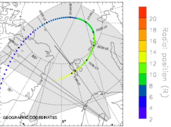
over-Fig. 2. Plot showing the geographical coverage of the ground-based instrumentation employed in this study, together with the magneti-cally mapped footprint of the Cluster 1 spacecraft. The grey areas show the fields-of-view of the CUTLASS radars, with the direc-tions of the centres of beams 1–3 and 8 of the Finland radar indi-cated. The heavy line and circled dot show the beam direction and location, respectively, of the steerable and fixed dishes of the EIS-CAT Svalbard radars. The coloured dots indicate the footprint of the Cluster 1 spacecraft at 5 min intervals, mapped magnetically to an altitude of 100 km using the Tsyganenko-96 model parameterised as in Fig. 1. The colour of the dot indicates the radial distance of the spacecraft, according to the code shown to the right of the plot.
laid on this path. The principal period of interest for this study is ∼ 09:00–11:00 UT, when the spacecraft were at ra-dial distances of ∼ 11–13 RE in the region of the
magne-topause. The locations of the remaining three Cluster space-craft (Salsa, Samba, and Tango) are also shown at each hour, although the inter-spacecraft separation has been magnified by a factor of ten relative to Cluster 1 in order to more easily display the tetrahedral geometry of the formation. Magne-tospheric field lines derived from the Tsyganenko-96 field model (Tsyganenko, 1995, 1996), that pass through the lo-cation of Cluster 1 at the one hour markers are represented by dotted lines (such lines are terminated when they reach the model magnetopause surface). The model is parame-terised by the solar wind dynamic pressure p, the IMF, and Dst. The values chosen here are p =1 nPa, IMF BY =5 nT,
IMF BZ = −3 nT, and Dst = −15 nT, corresponding to
prevailing conditions near the time of the boundary region encounter (∼ 09:30–10:30 UT). Finally, the solid lines indi-cate the location of the Tsyganenko-96 model magnetopause in the plane of each of the diagrams.
Each Cluster spacecraft is equipped with an identical pay-load comprising of eleven particle and field instruments. This study will draw upon measurements from one of these, name-ly the fluxgate magnetometer (FGM) experiment (Balogh et al., 1997). FGM is capable of providing high accuracy (up to 8 pT) vectors of the ambient magnetic field at high sam-ple rates (up to 67 vectors/s). For purposes of this study, however, all FGM data have been analysed at a temporal
res-olution equal to the spin period of the spacecraft (∼ 4 s). 2.2 ACE interplanetary data
Upstream solar wind and IMF conditions during the interval discussed in this paper were measured using the SWEPAM and MAG instruments, respectively, on the Advanced Com-position Explorer (ACE) spacecraft (McComas et al., 1998; Smith et al., 1998; Stone et al., 1998). During the relevant interval on 14 February 2001, ACE was located in the solar wind near the Sun-Earth L1 libration point, at GSM coordi-nates (X, Y, Z) = (+237.3, −37.6, +3.5) RE. The
propaga-tion delay between field signatures appearing at the space-craft and their arrival at the subsolar magnetopause has been estimated using the algorithm described by Khan and Cow-ley (1999). This algorithm takes into account the propaga-tion of IMF features from the solar wind to the bow shock and then across the magnetosheath to the magnetopause, using empirical model values of the location of the latter boundaries keyed to observed solar wind parameters. For conditions during the period of interest (nSW ∼1–3 cm−3,
VSW ∼500 km/s), the propagation delay is determined at
∼55 min, such that the ACE magnetometer data displayed below have been lagged by this interval for comparison with Cluster observations near the magnetopause.
2.3 CUTLASS radar data
Figure 2 illustrates the geographical coverage of the ground-based instruments employed in this study. Observations of ionospheric convection velocities are provided by the CUT-LASS radar system. This comprises of a pair of HF coherent-scatter radars located at Hankasalmi, Finland and Pykkvibær, Iceland, which form part of the international SuperDARN chain (Greenwald et al., 1995). Each radar is frequency agile (8–20 MHz), and routinely measures the line-of-sight (l-o-s) Doppler velocity, spectral width, and the backscatter power from ionospheric plasma irregularities. In normal operation (as here), the field-of-view (f-o-v) of each radar (shaded grey in Fig. 2) is formed by sequentially scanning through 16 beams of azimuthal separation 3.24◦, with each beam gated
into 75 ranges of 45 km length. The directions of the cen-tres of beams 1–3 and 8 of the Finland radar are indicated in Fig. 2 for future reference. Typically, the dwell time on each beam is 3 or 7 s, resulting in a scan of the complete f-o-v cov-ering 52◦ in azimuth and over 3000 km in range every 1 or 2 min. During the interval encompassed by this paper, both CUTLASS radars were operated in the higher time resolution mode, such that 1 min data is available.
Overlaid on Fig. 2 are the locations of the ionospheric field line footprints of the Cluster 1 spacecraft at 100 km altitude, obtained from the Tsyganenko-96 field mappings, parameterised as above. These are presented at 5 min inter-vals, each one colour-coded according to the scale on the right to indicate the radial position of the spacecraft. Fol-lowing perigee at ∼ 02:00 UT, the footprint travelled pole-ward over Greenland and into the north polar region,
be-fore beginning an equatorward and westward track through the CUTLASS fields-of-view that passed over the Svalbard archipelago at ∼ 10:30 UT. The spacecraft crossed the loca-tion of the model magnetopause at ∼ 11:35 UT, after which the field line tracing is terminated. The observations pre-sented below show that the magnetopause region was ac-tually crossed at ∼ 10:30 UT, with the implication that the spacecraft footprints were then located near Svalbard, cen-trally within the CUTLASS f-o-v. It is acknowledged that these model mappings become relatively less certain as the magnetopause is approached. However, as investigation has shown that the model magnetic field employed here is quite close to the field observed by Cluster. This lends some con-fidence that our mappings represent reasonable estimates for the purposes for which they have been employed.
2.4 EISCAT Svalbard radar data
The EISCAT Svalbard radar (ESR) facility at Longyear-byen (Wannberg et al., 1997), which operates at frequencies around 500 MHz, comprises of two separate co-located an-tennas, a fixed 42 m dish and a fully steerable 32 m dish. The fixed antenna is aligned along the local magnetic field direc-tion, which corresponds to a geographic azimuth of 181.0◦, with an elevation of 81.6◦. The location of the antenna is shown by the circled dot in Fig. 2. During the conjunction with the Cluster spacecraft, the steerable dish was directed northward at low elevation, with a geographic azimuth of 336.0◦, and an elevation of 30.0◦. The direction of the beam is indicated by the heavy black line in Fig. 2, which almost coincides with the CUTLASS Finland beam 8. Observations with a dwell time of 64 s were made alternately on each beam using an alternating code pulse scheme. The effective time resolution of the data on each beam was thus 128 s. Anal-ysis using the GUISDAP algorithm (Lehtinen and Huusko-nen, 1996) then provides estimates of the electron density, ion and electron temperature, and ion velocity, from the 90 to 1070 km range along each beam. Although this is approx-imately equivalent to the altitude coverage for observations along the near-vertical field-aligned beam, the low elevation observations span some 50 to 600 km in altitude, with a lati-tude coverage indicated by the length of the black line shown in Fig. 2.
3 Observations
3.1 Cluster data
In Fig. 3, we display ACE and Cluster magnetic field data for the two-hour interval of 09:15 to 11:15 UT on 14 February 2001, which encompasses the outbound Cluster transition between the magnetosphere and magnetosheath. The up-per panels show the GSM components of the IMF, measured upstream of the Earth by the ACE spacecraft. The data are shown at 16 s resolution, and have been lagged by 55 min to the subsolar magnetopause, as indicated above. The up-stream IMF was directed nearly continuously southward
dur-ing the interval, with BZ∼ −3 nT, having turned from
north-ward values at a (lagged) time of 08:53 UT. The IMF also had weaker positive Y (∼ 5 nT) and near-zero X components which became more variable after ∼ 10:30 UT.
Beneath the IMF data we show Cluster magnetometer data. The data are presented with a 4 s resolution, and for initial clarity, we show data only from Cluster 1 (Rumba). The data from the other Cluster spacecraft show similar fea-tures, as we will indicate below. The top three panels of Cluster data show the three field components in boundary normal coordinates (Russell and Elphic, 1978), where N is the estimated outward normal to the magnetopause, L lies in the boundary and points north (such that the L − N plane contains the GSM Z-axis), and M also lies in the boundary and points west, orthogonal to L and N (such that (L, M, N ) forms a right-handed coordinate system). Note that the scale of the panel showing the N component is half that of the pan-els showing the L and M components, in order that the vari-ations in BNcan be clearly seen. Beneath these, we show the
total field strength, and the angle of the field in the plane of the magnetopause, αLM, defined as αLM =arctan(BM/BL).
Finally, at the foot of the figure, we show position data for the spacecraft, specifically the geocentric radial distance (RE),
and the GSM local time and latitude. We note for future reference that the magnetopause crossings near the centre of the interval occurred at a radial distance of ∼12 RE, a
post-noon GSM local time of ∼ 14.2 h, and a GSM latitude of ∼61◦. In fact, this location is very close to that at which the original “flux erosion events” were observed by Haerendel et al. (1978) in HEOS-2 data (at ∼ 13 RE, ∼ 13.6 h, and ∼ 64◦,
see also Rijnbeek and Cowley, 1984).
The outward magnetopause normal for the Cluster data has been determined by minimum variance analysis of the Cluster 1 data during the interval of 10:00–10:40 UT, an in-terval which contains the boundary layer traversal and all three magnetopause transitions. This normal is thus taken to be representative of the boundary region as a whole. In-vestigation shows that near similar directions are obtained from the data from all four Cluster spacecraft over the in-terval, and that the direction is also relatively insensitive to the precise interval analysed. For all four spacecraft, the difference in magnitude between the intermediate and mini-mum eigenvalues of the covariance matrix was found to be a factor of ∼ 8, indicating that the calculated minimum vari-ance direction was robust in each case. Furthermore, much shorter (5 min) intervals were also investigated spanning each of the magnetopause transitions. In each case, the normals determined from each spacecraft were found to be consis-tent, and to differ in direction by less than ∼ 20◦from that given above for the whole boundary region. Such differences produce essentially no qualitative change in the boundary normal coordinate data plots. Therefore, we have adopted here the outward normal direction determined from the inter-val of 10:00–10:40 UT, given by GSM components (+0.669, −0.262, +0.696). The comparable positive X and Z com-ponents seem reasonable for a magnetopause transition at high-latitudes in the vicinity of the cusp (see the model shape
Figure 3
Fig. 3. Plot of the magnetic field observations made by the ACE and Cluster 1 (Rumba) spacecraft during the interval 09:15–11:15 UT on 14 February 2001. The top three panels show the GSM components of the upstream IMF measured by the ACE spacecraft, lagged by 55 min to the subsolar magnetopause. These data are shown at 16 s resolution. The following panels then show the three components of the Cluster 1 magnetic field in boundary normal coordinates (see text), the field magnitude, and the angle of the field in the plane of the magnetopause relative to the GSM northward direction, αLM. These data are at spacecraft spin (∼ 4 s) resolution. At the foot of the figure,
we show Cluster 1 position data, specifically the geocentric radial distance, and GSM local time and latitude. The vertical dashed lines indicate times of particular interest, namely the centres of flux transfer events (FTEs), the inner edge of the magnetopause boundary layer (BL), and magnetopause current sheet crossings (MP).
shown in Fig. 1), while the small, negative Y component is perhaps surprising for a post-noon transition. However, the negative Y component is consistently present in the normals determined from each spacecraft, and for the various inter-vals investigated. It suggests that the magnetopause surface is significantly dimpled inwards in the vicinity of the cusp at noon, such that the boundary normal in the immediate high-latitude post-noon sector (∼ 14.2 hr GSM MLT for this cross-ing) is deflected modestly towards dawn. A similar orienta-tion of the post-noon magnetopause was found previously by Rijnbeek and Cowley (1984) in the study of the HEOS-2 high-latitude “flux erosion events” mentioned above (the GSM normal vector in that case was determined as (+0.649, −0.081, +0.757)).
At the beginning of the interval shown in Fig. 3, the space-craft was located within the magnetosphere where the field strength was ∼ 20 nT and directed principally southward and westward (BLnegative, BM positive). As the magnetopause
was approached, however, the L component drifted towards near-zero and in a positive (northward) direction. At the end of the interval, the spacecraft was located in the mag-netosheath where the field was still ∼ 20 nT, but much more rapidly varying, and directed southward and eastward (BL
and BM are negative). The latter directions are qualitatively
consistent with the expectations based on the upstream IMF direction. Three principal magnetopause boundary cross-ings have been identified, indicated by the vertical dashed lines marked “MP”. These occur at ∼ 10:17, ∼ 10:22, and ∼10:33 UT and, as indicated above, mark transitions be-tween fields on the magnetospheric side which have (primar-ily) positive L and M components, and fields on the mag-netosheath side which have (primarily) negative L and M components.
During the initial magnetospheric interval, prior to the first magnetopause encounter, the field became increasingly vari-able in both direction and magnitude as the magnetopause was approached. These variations appear to have begun near ∼09:00 UT, shortly after the (lagged) IMF turned southward at the subsolar magnetopause. It seems clear that this vari-ability was connected with ongoing dynamic phenomena in the boundary region. These field variations culminated in the ∼30 min interval prior to the first magnetopause encounter, with the observation of four clear magnetospheric FTEs, cen-tred near ∼ 09:45, ∼ 09:54, ∼ 09:59, and ∼ 10:04 UT, which are also marked by dashed vertical lines. These FTEs are all indicated by bipolar positive-to-negative (“normal” polarity) excursions in the N component of the field, together with in-creases in the field strength. We also note that the first of these FTEs appears to have been preceded and followed by smaller amplitude perturbations of a similar kind. The varia-tion in αLM shows that the field direction in the plane of the
magnetopause rotated away from the magnetosheath field di-rection at the spacecraft in the first FTE. The field didi-rection did not rotate significantly in the second FTE, but did ro-tate through a small angle towards the magnetosheath field direction in the third FTE, and underwent a large rotation to-wards the magnetosheath field direction in the fourth FTE.
The latter rotation was associated with a large increase in BLfrom near-zero outside the event to ∼25 nT inside, while
the BMcomponent underwent a simultaneous reduction from
∼15 nT outside the event to ∼ −5 nT inside. In effect, the field in the plane of the magnetopause rotated through ∼90◦ from a magnetospheric near-westward orientation to point northward and slightly eastward. We note that the sense of the latter perturbations is very similar to those of the “flux erosion events” observed by HEOS-2 at a similar location under similar magnetosheath circumstances.
After the observation of the four magnetospheric FTEs, the spacecraft entered a magnetopause boundary layer at ∼10:09 UT, which endured until the first magnetopause crossing at ∼ 10:17 UT. Although highly variable, the direc-tion of the field in this layer was generally similar to that within the centre of the final clear FTE, i.e. it was directed northward and eastward, sheared towards the direction of the field in the magnetosheath. The field strength was also vari-able, but significantly elevated over that found in both the magnetosphere and magnetosheath, reaching peak values of ∼50 nT. Following the transition into the magnetosheath at ∼10:17 UT, the spacecraft then briefly re-entered the mag-netosphere between ∼ 10:22 and ∼ 10:33 UT. In these cases, the magnetopause transitions were relatively rapid and as-sociated with brief spike-like perturbations in all three field components. However, only modest field perturbations were observed within the brief magnetospheric interval, with no FTEs. In the following traversal of the magnetosheath, how-ever, FTEs were again observed. Two prominent exam-ples are centred near ∼ 10:46 and ∼ 11:01 UT, with events of smaller amplitude occurring at ∼ 10:36 and ∼ 10:43 UT. These are also indicated by dashed vertical lines, and show “normal” polarity bipolar signatures in the N field compo-nent, together with variable tilting effects in the plane of the magnetopause. Other FTE-type field structures may also be present in the magnetosheath, associated with small ampli-tude or shorter-lived field features.
Our interpretation of the field perturbations observed dur-ing these FTE events is sketched in Fig. 4. In Fig. 4a, we show a cut in a magnetic meridian in the noon sector a few minutes after a burst of reconnection has occurred at low-latitudes. A bulge of newly-reconnected field lines propa-gates over the magnetopause towards the cusp, and from then on into the tail lobe. Its passage is marked by a bipolar sig-nature in the N field component in both the magnetosphere and the magnetosheath, in which the field first points out-wards and then inout-wards, as observed. The size of the bulge (for a large amplitude FTE) is ∼ 1 RE normal to the
mag-netopause (Saunders et al., 1984), and several RE along the
magnetopause in the plane of the diagram (such that with a propagation speed over the magnetopause of a few hun-dred km/s, the propagation time across a given point will be ∼1–2 min). Of course, in the presence of a significant BY
component in the IMF, positive in the present case, the re-connected field lines will not lie directly in the plane of this diagram, but will be tilted out of the plane by the effect of the field tension. This is indicated by the field component
di-rected out of the plane of the diagram which has been drawn within the FTE (and which is also present, of course, in the magnetosheath).
Field tilting effects in the plane of the magnetopause are shown more clearly in Fig. 4b. This shows a sketch of the dayside magnetopause viewed from the Sun, where the ar-rowed dashed lines show undisturbed magnetospheric field lines in the magnetopause layer. The arrowed solid lines show individual field lines of a given FTE at a fixed instant of time, which originated from a propagating burst of low-latitude reconnection. Specifically, in line with the recent observations presented by Milan et al. (2000), we assume that reconnection starts in a burst close to the noon merid-ian, giving rise to field line “1” (plus neighbouring open field lines), and then propagates to later local times, giving rise sequentially to field lines “2”, “3”, and “4”. The latter field lines have thus undergone sequentially less evolution over the magnetopause since reconnection, originating from re-connection sites displaced increasingly duskward of noon. Thus, field line “4”, for example, has only just been recon-nected at the time of the figure, thus marking the approxi-mate location of the reconnection region at that time. Field lines reconnected earlier, closer to noon, are relatively more evolved. The reconnection region may also propagate simul-taneously dawnward from noon to earlier local times as well, but the effect of this (giving rise to “younger” open tubes on the dawn flank as well) has not been represented in the figure. After reconnection has taken place, the combined ac-tion of the magnetic tension of the newly-opened field lines and magnetosheath flow causes them to contract poleward and westward (for positive IMF BY) as indicated, forming
a sunward-moving boundary layer in the post-noon topause, as described, for example, by the simple magne-topause reconnection model of Cowley and Owen (1989). As can then be seen, the effect of the field tension is such that it causes the newly-opened magnetospheric flux tubes to rotate towards a poleward and eastward orientation. In other words, the field direction in the high-latitude magne-tospheric boundary region at Cluster (shown in the figure by the spacecraft symbol) should rotate clockwise in the plane of the magnetopause, from positive M towards positive L and negative M. This scenario is thus qualitatively consis-tent with the sense of the principal FTE and boundary layer field perturbations seen in Fig. 3. The “reversed” and reduced field tilting effects observed in the first three magnetospheric FTEs marked in the figure, as compared with the fourth, is due to the larger distances from the magnetopause in the ear-lier events, combined with a twisting of the field within the FTE structure, as previously discussed, for example, by Cow-ley (1982), Paschmann et al. (1982), Saunders et al. (1984), Southwood et al. (1988), and Wright and Berger (1989). The twisting is often such that in the outer part of the FTE, the field may tilt away from the direction of the field on the other side of the boundary. Such tilts can also be produced in the unreconnected field immediately outside the FTE due to the flows induced in the surrounding medium by the passage of the FTE structure (Southwood, 1985; Cowley, 1986).
The shearing of the field within the FTE structures can also be seen directly in the four spacecraft Cluster magne-tometer data. In Fig. 5, we show such data for the magneto-spheric boundary region on an expanded time base (09:40– 10:20 UT), using the same boundary normal coordinate sys-tem as in Fig. 3 (this was determined specifically from Clus-ter 1 data as indicated above, but the minimum variance directions determined individually from all four spacecraft were essentially identical). The vertical lines show the same principal times as in Fig. 3. The purple line corresponds to data from Cluster 1 (Rumba), green to Cluster 2 (Salsa), yel-low to Cluster 3 (Samba), and red to Cluster 4 (Tango) (the same colour-coding as in Fig. 1). Assuming that the distance from the magnetopause is the principal organising parameter, we note that Clusters 1–3 lie roughly in the same plane as the estimated plane of the magnetopause (within ∼ 60 km, i.e. within ∼ 0.01 RE), while Cluster 4 lags behind these
space-craft by ∼ 510 km (∼ 0.08 RE) along the boundary normal.
The relatively small values of these displacements indicate that only small-scale structures, with field variations on the scale of ∼ 0.1 RE, or less, will result in marked differences
in the field between the spacecraft. As indicated above, the spatial scale of large amplitude FTEs transverse to the mag-netopause is ∼ 1 RE. Only relatively minor differences in
the field values between the spacecraft are then expected for structures of such size.
Examination of Fig. 5 shows that in general the latter ex-pectation is fulfilled (though, of course, the small differen-ces observed will be vital to future detailed modelling stud-ies). Careful examination of the data shows, however, that in general, the field variations of Clusters 1–3 (purple, yellow, and green) track each other very well during the FTE events, while Cluster 4 shows a somewhat more markedly differ-ent behaviour, with field perturbations of a smaller ampli-tude (see particularly the second to fourth FTEs). Within the boundary layer, however, we note the presence of field struc-tures in which zero-order differences in the field occurred be-tween the four spacecraft, particularly during the interval of ∼10:09–10:13 UT. In these structures, the largest field shear-ing perturbations in the estimated plane of the magnetopause were observed by Cluster 1, followed in order by 3, 2, and 4. This ordering is not expected for a structure which simply propagates along the magnetopause normal in the orientation determined here; therefore, further study of the structure and geometry of these events is warranted. We may already con-clude from these data, however, that the observed structures were that of an FTE-like open flux tube, with a spatial scale of ∼ 0.1 RE perpendicular to the magnetopause,
compara-ble to the normal separation of the Cluster spacecraft. The other FTE events noted here must clearly have had signif-icantly larger spatial scales than this, as will be elucidated with further study of these data. The most reasonable picture of the boundary layer identified in these observations is that it was formed from nearly continuous but highly variable re-connection at the magnetopause, in which the FTEs observed at larger distances represent the large-scale peaks extending further from the boundary. The field strength increases
ob-J. A. Wild et al.: First simultaneous observations of flux transfer events at the high-latitude magnetopause 1499
X
Z
By1
2
3
4
(a)
(b)
L
N
M
Figure 4X
By 1 2 3 4(a)
(b)
L N M Figure 4Fig. 4. Sketches illustrating the magnetic field effects produced by a propagating burst of magnetopause reconnection. (a) View in a near-noon magnetic meridian plane showing the effects produced by a burst of low-latitude reconnection in that meridian. A bulge of newly-reconnected open flux tubes propagate poleward to the cusp, and from there into the tail. The open field lines are also twisted out of the meridian by the Y component of the IMF, associated with the field component pointing out of the plane of the diagram marked BY as shown (which is
also present, of course, in the magnetosheath outside). The local boundary normal coordinate directions are also indicated, such that it can be seen that the passage of the bulge will give rise to a bipolar signature in the N component. The dashed line beneath the bulge indicates the tangential discontinuity magnetopause remaining after the bulge has passed by. (b) View of the Earth’s dayside magnetopause looking from the Sun, showing individual field lines at one instant of time (solid lines with arrows) which were produced by a propagating burst of reconnection. Collectively, these open lines constitute a given FTE. We assume that the reconnection burst started near noon (producing field line “1”), and then propagated towards dusk, producing field lines “2”, “3”, and “4” in sequence. “Later” field lines (like “3” and “4”) have thus undergone less evolution over the magnetopause since reconnection than “earlier” field lines (line “1” and “2”). Field line “4” has only just been reconnected at the time shown, thus marking the eastward boundary of the reconnection region at that time. The effect of a similar progress from noon towards dawn has not been represented. The short-dashed lines with arrows indicate undisturbed magnetospheric field lines within the magnetospheric boundary region. The long-dashed lines indicate the latitudes of the equator (lower line) and cusp (upper line). The field tension effect on the open flux tubes is to cause them to contract poleward and dawnward over the magnetopause, as shown by the arrows, such that the field in the high-latitude post-noon boundary layer at Cluster (shown by the spacecraft symbol) tilts clockwise from westward towards northward and eastward orientations.
served both in the FTEs and in the boundary layer structures serve to emphasise the essentially 3-D nature of these phe-nomena. The increases in field (and total) pressure are due to the effect of the field tension of the overlying (and under-lying) field lines, and of the field twisting inside the struc-tures. In near slab-like magnetopause structures, the total pressure would be preserved in passing through the bound-ary, and large increases in field pressure as observed here would not be expected.
3.2 CUTLASS radar data
The Cluster data presented above indicate the presence of pulsed reconnection at the dusk magnetopause which per-turbs the field in the high-latitude boundary region, both in the magnetosphere and magnetosheath. We have previously seen in Fig. 2 that these boundary field lines are expected to map magnetically to the central portion of the fields-of-view of the CUTLASS radars, and also close to the beams of the
EISCAT Svalbard radar. In this section, we now examine the concurrent radar data.
During the interval of interest, both CUTLASS radars were observing the dayside auroral zone close to local noon, as indicated above. Fig. 6 shows the backscatter observed by the radars in a geomagnetic latitude and MLT format where the dashed radial lines show one hour intervals of local time (noon being vertical), and the concentric dashed circles indi-cate magnetic latitudes of 70◦and 80◦. The solid lines
indi-cate a statistical auroral oval, and the black dot is the mapped Cluster footprint. Data are shown at two times. The first is 09:50 UT, close to the start of the interval during which Cluster observed magnetospheric FTEs when the spacecraft footprint was located approximately 1 h MLT to the east of Svalbard. The second is 10:37 UT, shortly after the last Clus-ter traversal of the magnetopause when the mapped footprint was co-located with Svalbard. At 09:50 UT, backscatter was observed by both CUTLASS radars (Figs. 6a and b), but
Figure 5
Fig. 5. Four spacecraft Cluster magnetometer data for the interval 09:40–10:20 UT are shown in boundary normal coordinates in the same format as in Fig. 3. The coordinate system is also the same as in Fig. 3. Data from Cluster 1, 2, 3, and 4 are shown by the purple, green, yellow, and red lines, respectively. The vertical dashed lines indicate the FTEs, boundary layer inner edge (BL), and magnetopause crossings (MP), as in Fig. 3.
only the Finland radar observed backscatter of significance at 10:37 UT (Fig. 6c). The radar backscatter is colour-coded as Doppler velocity, i.e. the line-of-sight component of the bulk plasma drift. Positive velocities represent motion towards the radar. Regions colour-coded grey indicate backscatter echoes with low Doppler velocity and low Doppler spread, which are generally interpreted as backscatter from the ground.
The Finland radar observations at 09:50 UT (Fig. 6a) show two main regions of ionospheric backscatter, one at lower lat-itudes (∼75◦geomagnetic) and the second at higher latitudes (poleward of 80◦latitude). Unfortunately, the first is embed-ded within or superimposed on a region of ground backscat-ter, which often means that the ACF analysis technique em-ployed by the SuperDARN radars may have had trouble cor-rectly measuring the Doppler velocity. In the present case, however, the measurements do not appear to be affected. In the western and eastern portions of the field-of-view, the line-of-sight velocity is directed away from and towards the radar,
respectively, indicating that the flow here has a significant westward azimuthal component. Indeed, a beam-swinging analysis of the velocities indicates that they are most consis-tent with a flow of 400 m/s, directed 70◦to the west of ge-omagnetic north. The westward flow direction is consistent with the plasma drift expected in the cusp region for posi-tive IMF BY (the “Svalgaard-Mansurov effect”), as is indeed
observed in the lagged IMF data from the ACE spacecraft (see Fig. 3). It is also consistent with the anticipated mo-tion of the northern hemisphere open flux tubes shown above in Fig. 4b (see the grey arrows in the vicinity of the cusp). Physically, the westward motion is due to the effect of the magnetic field tension associated with positive IMF BY, as
indicated above. The second main region of backscatter lies within the polar cap and shows relatively low flow velocities. These flows will be described further below, in conjunction with ESR observations. The CUTLASS Iceland observations from this time (Fig. 6b) are consistent with the description of
Figure 6
Fig. 6. Three panels illustrating the line-of-sight velocity measurements made by the (a) Finland and (b) Iceland CUTLASS radars at 09:50 UT and (c) at 10:37 UT. The data are shown on a geomagnetic grid, with noon at the top and 70◦and 80◦latitude circles (dashed lines) shown. The solid lines show a statistical auroral oval, while the magnetically mapped Cluster footprint is shown by the black dot.
the Finland measurements. At the latitude of Svalbard where there is overlap with backscatter in the Finland radar field-of-view, the Iceland radar recorded positive Doppler shifts, consistent with westward flow. Just to the west of this is a region of negative Doppler shifts, possibly indicating return flow in the dawn convection cell.
Turning to the observations from 10:37 UT (Fig. 6c), the lower latitude region of backscatter is still present. The pat-tern of line-of-sight velocities within this region remains un-changed, i.e. the flow is still directed predominantly west-wards. However, beam-swinging shows that the speed has increased to be closer to 800 m/s. A succession of beam-swinging analyses of the Doppler shifts within this region of backscatter indicates that the flow magnitude increases grad-ually from near 300 m/s at 09:40 UT, to 800 m/s at 10:25 UT, after which it remains constant until the backscatter echoes disappear at 10:45 UT. However, this behaviour is indicative of the behaviour of the background flow on large spatial and temporal scales, and does not preclude the possibility of sig-nificant smaller scale features that could be associated with the FTEs observed by Cluster. In addition to the westward flow region, a new region of backscatter is also observed in Fig. 6c in the western portion of the field-of-view of the radar. These echoes have high Doppler shifts directed away from the radar, suggestive of a significant poleward component to the plasma drift. It is backscatter of this nature which has previously comprised the main radar signature of transient and impulsive flux transfer.
Figure 7 concentrates on the Finland radar observations in the western portion of the field-of-view. Although these data are obtained from locations displaced by ∼ 2 h MLT west of the estimated footprint of Cluster (Fig. 6), the direction of the beams ensures that the line-of-sight velocities are re-sponsive to the dominant east-west component of the flow in the lower latitude backscatter band. In general, we ex-pect that large amplitude events, such as those investigated here, should produce flow effects in the ionosphere of suffi-ciently large enough spatial scale that related effects will still
be observed at such displacements (e.g. Milan et al., 2000). In the upper panels of Fig. 7, we thus show magnetic lat-itude time plots of backscatter power and Doppler velocity for beams 1, 2, and 3 (see Fig. 2), for the period of 09:15 to 11:15 UT (as for the Cluster data in Fig. 3). Note that the velocity colour scale employed in Fig. 7 is different from that in Fig. 6. Since all flows observed in these beams dur-ing this interval are directed away from the radar, only neg-ative Doppler shifts are shown. At lower latitudes, a region of ground backscatter is seen between 09:30 and 10:30 UT in all three beams. Just poleward of this, between the lati-tudes of 74◦and 76◦, relatively low Doppler shift ionospheric backscatter is observed, corresponding to the region of west-ward flows identified in Fig. 6. Polewest-ward of this, again above 76◦ in latitude, higher Doppler shifts are present. Again, it is these echoes which, in the past, have been identified as the radar signature of FTEs. Pinnock et al. (1995) and Provan et al. (1998) described the radar signature of FTEs as “pulsed ionospheric flows” or PIFs, i.e. poleward-moving regions of enhanced convection flow in the dayside auroral zone. These are often also seen as poleward-moving re-gions of backscatter or enhanced backscatter power, the radar counterpart of “poleward-moving auroral forms” (PMAFs), widely accepted to be the auroral signature of FTEs (e.g. Sandholt et al., 1990; Thorolfsson et al., 2000). In the fol-lowing discussion we will refer to these radar PMAFs as “poleward-moving radar auroral forms” or PMRAFs. (As a slight digression, we note that care should be taken in the use of “PIF” and “PMRAF” nomenclature, which are of-ten erroneously used interchangeably, i.e. it is not possible to say whether or not isolated PMRAFs are associated with a PIF since no measurements of the ionospheric flow pre-ceding or following the PMRAF are made (as no backscat-ter is observed). The lack of backscatbackscat-ter before or afbackscat-ter the PMRAF does not necessarily indicate that a change in con-vection flow has occurred, only that no targets were present from which the radar could scatter.) Depending on the ex-act nature of the convection response to transient
reconnec-Figure 7
Fig. 7. Three pairs of backscatter power and Doppler shift measurements from beams 1, 2, and 3 of the Fin-land radar are shown, covering the same time interval as for the Cluster data in Fig. 3. In the power panels, black indicates an insufficient signal-to-noise ratio used to determine the spectral characteristics of the backscatter. In the Doppler shift panels, velocities are only shown where significant power is observed. Grey backscatter indicates ground backscatter, and negative ve-locities represent Doppler shifts away from the radar along the line-of-sight. Poleward-moving radar auroral forms (PMRAFs) are indicated by arrows in the upper (beam 1) power panel; re-lated events are observed in each of the other beams shown. Superimposed on each panel are the times identified in the Cluster observations, as in Fig. 3, specifically, the centre times of the four magnetospheric FTEs, the entry into the boundary layer (BL), the three cross-ings of the magnetopause (MP), and the four magnetosheath FTEs.
tion, either PIFs (Pinnock et al., 1995) or PMRAFs (Milan et al., 2000), or both (Provan et al., 1998) can be observed by SuperDARN radars. In the present case, both are ob-served. Two clear examples of PMRAFs are seen at 09:21– 09:26 UT and 09:41–09:45 UT in beams 1 to 3, marked by the arrows in the upper panel. In these examples, a narrow region of backscatter containing negative Doppler shifts is seen to progress poleward over a latitudinal range of ∼ 2◦in
the space of a few minutes. Examples of events which can be identified as both PIFs and PMRAFs are seen between 10:30 and 10:50 UT. Here, a continuous region of backscat-ter is seen, but within this are several poleward-moving en-hancements in the backscatter power (see especially beam 1). Simultaneously, the Doppler shifts are modulated such that the enhanced power features are associated with elevated Doppler shifts. In all, four such events are seen in this 20 min interval. The middle two events form the high Doppler shift region identified in Fig. 6c. These and other PMRAFs which occur during the interval are also marked by arrows in the upper panel of the figure.
Over and above these PIFs and PMRAFs, the present ob-servations, in conjunction with the Cluster magnetopause measurements, allow us to gain new insight into the
pro-cesses which give rise to these “traditional” signatures of FTEs. The PIF/PMRAF signatures are primarily identified in the higher latitude backscatter region, i.e. that region con-taining high Doppler shifts. However, there is also evidence that the backscatter power and velocity are modulated in the lower latitude ionospheric backscatter region corresponding to westward flow, and we recall from Fig. 6 that it is in this lower latitude region that the magnetically mapped Cluster footprint lies. In association with the first, second, and fourth magnetosphere FTEs identified in the Cluster measurements, there appear to be enhancements in the power of this low-latitude backscatter, especially in beam 2. These power en-hancements are seen to start at 09:45, 09:54, and 10:05 UT, and have a duration of approximately 5 min. Other simi-lar enhancements are observed at 10:14, 10:21, 10:32, and 10:40 UT. In addition, the Doppler shifts within this region of backscatter also appear modulated, with increases in the velocity corresponding to enhancements in power.
The velocity modulation is not wholly clear from the colour scale employed in Fig. 7, so in the upper panel of Fig. 8, we reproduce the velocity measurements of beam 3 on a more suitable scale, and compare them with the Cluster data. Beam 3 has been chosen since this has the longest
un-Figure 8
Fig. 8. The upper panel shows CUT-LASS Finland velocity data from beam 3, in a similar format to Fig. 7, but with a revised colour scale which reveals the pulsing of the line-of-sight flow in the band of lower latitude scatter. The sec-ond panel shows the mean velocity ob-served in this band, averaged over the latitude range located between the hor-izontal dashed lines in the upper panel (and given a positive value in this case, though the flow is directed away from the radar). The lower panel shows the BNfield component observed by
Clus-ter 1, as in Fig. 3. The vertical dashed lines are as in Figs. 3 and 7.
broken series of measurements in the lower latitude backscat-ter region. The second panel in Fig. 8 shows a time-series of the Doppler shift measurements from the lower latitude backscatter region of this beam, averaged between the hor-izontal dashed lines in the top panel (∼ 74.5◦–76◦ mag-netic latitude). The line-of-sight flow is seen to be char-acteristically pulsed from ∼ 100 to ∼ 300 m/s on 5–10 min time scales, in approximate concert with the pulsing of the backscatter power. The third panel in Fig. 8 reproduces the BN component of the Cluster magnetometer data,
contain-ing the principal FTE signatures, for purposes of detailed comparison. It can be seen that enhancements in the ve-locity occur in association with each of the four magneto-spheric FTEs, with peak values occurring typically 1–2 min after what has been judged to be the “centre” time of the Cluster FTEs, shown by the vertical dashed lines. The rela-tive timing of such pulses for individual events will depend upon the relative propagation times from the reconnection site over the magnetopause to the spacecraft, and along the field to the ionosphere and from then on to the radar field-of-view. Each of these propagation times will typically be of the order of a few minutes (∼ 1–5 min, say), such that ∼ 1–2 min displacements in either direction are not unexpected, depend-ing upon the details. Flow enhancements are also observed following the occurrence of large amplitude BN signatures
in the boundary layer, in association with the final magne-topause crossings (which also have spike-like BNsignatures,
as noted above), and in association with the magnetosheath FTEs, though we note that the velocity measurements at the latter time are patchy and noisy.
We find, therefore, a compelling association between FTE signatures observed at the magnetopause with enhancements in velocity and power observed in the backscatter echoes, corresponding to the lower latitude westward flow region, i.e. flow that is consistent with the expected motion of
re-cently reconnected flux tubes. This correspondence is good despite the fact that these ground-based measurements are made ∼ 2 h MLT to the west of the Cluster footprint. Unfor-tunately, we cannot make similar measurements directly con-jugate with Cluster, since here the westward flow is nearly perpendicular to the radar beam look-directions (Fig. 2), and thus, no clear modulation of the line-of-sight velocity is ob-served (see Fig. 9 below). However, we noted above that these events and their ground-based signatures are, in gen-eral, likely to be large in spatial scale, and our results confirm this expectation. Some ground-based events do occur with-out a clear signature at the spacecraft, such as the PMRAFs observed at ∼ 09:21 and ∼ 09:41 UT. However, the space-craft was only approaching the boundary region during that interval, and was presumably too far from the magnetopause to observe the related FTE signatures.
These observations thus suggest that the lower latitude westward flow region observed here corresponds to newly-opened flux tubes in which the first influences of each burst of reconnection is felt. Therefore, it is of interest to con-sider the relationship between the flow and power enhance-ments observed in this region with the PIF and PMRAF sig-natures observed at higher latitudes. Examination of the data in Figs. 7 and 8 shows that these are closely related. The observations in beam 2, for example, suggest that each en-hancement in backscatter power observed in the westward flow region between 10:05 and 10:45 UT precedes a PIF or PMRAF signature in the higher latitude backscatter. In other words, the PIF/PMRAF events originate near a latitude of 74◦–75◦, mapping close to the latitude of the Cluster foot-print, and propagating poleward close to the 80◦ latitude where they resemble the more classic PIF/PMRAF signa-tures. We note that a delay of a few minutes can be asso-ciated with this poleward propagation. This association be-tween flow changes at lower latitudes and PMRAF features at
79 80 81 82 Magnetic Latitude 79 80 81 82 Magnetic Latitude -800 -600 -400 -200 0 200 400 600 800 Ion V elocity (ms -1 ) 200 300 400 500 600 700 Altitude (km) 200 300 400 500 600 700 Altitude (km) 0.0 0.8 1.6 2.4 3.2 4.0 4.8 5.6 6.4 7.2 Electron Density (x10 11 m -3 ) 0920 0940 1000 1020 1040 1100 UT 100 200 300 400 500 600 700 Altitude (km) 0920 0940 1000 1020 1040 1100 UT 100 200 300 400 500 600 700 Altitude (km) 0 300 600 900 1200 1500 1800 2100 2400 2700 Ion T emperature (K) 75 80 85 Magnetic Latitude 75 80 85 Magnetic Latitude -800 -600 -400 -200 0 200 400 600 800 V elocity (ms -1 ) Ground Scatter
FTE FTE FTE FTE BL MP MP MP FTE FTE FTE FTE
Beam 8
Figure 9
Fig. 9. EISCAT Svalbard radar data for the same time interval as shown for the Cluster data in Fig. 3 and the CUTLASS Finland radar data in Fig. 7. The upper panel shows CUTLASS Finland velocity measurements from beam 8 for purposes of comparison. The second panel shows the latitudinal variation in line-of-sight ion velocity measured by the steerable dish of the ESR. In both the upper and second panels, positive and negative line-of-sight velocities represent motion toward and away from the radars, respectively. The third and fourth panels show the electron density and ion temperature, respectively, measured along the field-aligned ESR beam. All ESR data are shown at a 128 s resolution. The vertical lines show the same key times from the Cluster data as shown in the previous time-series plots.
higher latitudes was previously found in the study presented by Milan et al. (2000). Recent work suggests that the iono-spheric electron density is structured in response to changes in flow excited by transient reconnection (i.e. in the west-ward flow region) and that these electron density structures then propagate poleward, embedded within the background convection flow. The electron density gradients associated with these structures drive plasma instability processes which produce ionospheric irregularities, the targets from which SuperDARN radars scatter (see, for instance, Milan et al., 1999a). Since the recombination rate in the F-region iono-sphere is low, these electron density gradients can persist for many tens of minutes as they convect in the background flow. However, the instability growth rate is governed by the scale-length and size of these gradients which, in turn, is controlled by the details of the structuring mechanism which first pro-duced them, i.e. significant backscatter may or may not be as-sociated with any particular event depending on exactly how this structuring took place. These variations presumably ac-count for the fact that some of the lower latitude pulses are associated with PIF/PMRAFs, while others are not. If ir-regularities are produced, however, they may well persist for longer than they are observed by the radar, with the latter interval controlled by instrumental factors, such as the max-imum range to which the radar illuminates the ionosphere.
Therefore, PMRAFs are fossils of the ionospheric structur-ing that takes place at the ionospheric footprint of the merg-ing gap. The discrete nature of these fossils relates to the impulsive nature of the flow-excitation process. These fos-sils thus provide an excellent tracer of the convection flow on newly-reconnected field lines, excited by the reconnec-tion process poleward of the merging gap. Whether these fossils are associated with PIFs, i.e. is modulations in the ionospheric flow, or not gives us a clue as to the level that oc-curs of inductive smoothing of the flow, excited by the recon-nection process. One important repercussion of this picture is that the observation of a PMRAF may be delayed from its associated burst of reconnection by up to several min-utes. This is consistent with the observations in the present interval. It is not clear from the observations what process gives rise to the enhancements in backscatter power seen in the lower latitude backscatter, though we assume that these are directly related to bursts of reconnection occurring at the magnetopause. The enhancements in the ionospheric elec-tron density through precipitation, driven by the reconnec-tion process, are one possible source. Such enhancements in the background electron density would give rise to an in-crease in the irregularity scatter cross section which controls the backscatter power.
3.3 EISCAT Svalbard radar data
The observations discussed above suggest that during the in-terval investigated here, the ionosphere above Svalbard, con-jugate to Cluster, was subject to impulsive flows and precip-itation associated with FTE-related bursts of magnetopause reconnection. Therefore, it is of interest to briefly
exam-ine the ionospheric structure which resulted from these pro-cesses. Fig. 9 thus shows ESR observations from 09:15 to 11:15 UT (as in the previous diagrams). The upper panel also illustrates line-of-sight irregularity drift velocity mea-surements from beam 8 of the Finland radar as a function of magnetic latitude from 70◦ to 87◦ (see Fig. 2), shown for purposes of comparison. As in previous figures, posi-tive and negaposi-tive velocities represent motion of irregularities toward and away from the radar, respectively, while returns attributed to ground scatter are indicated in grey. The sec-ond panel presents line-of-sight ion velocity estimates at a 128 s effective resolution from the low elevation northward-directed ESR beam (azimuth 336◦, elevation 30◦). The di-rection of this beam lies close to that of the CUTLASS Fin-land beam 8, as can be seen in Fig. 2. These data are again shown as a function of magnetic latitude, but this time, be-tween 78◦and 82◦; the observations cover the F-region
al-titude range between 200 and 530 km. The third and fourth panels present 2 min resolution observations of electron den-sity and ion temperature, respectively, from the field-aligned ESR beam (azimuth 181◦, elevation 81.6◦), as a function of altitude from 100 to 700 km. It is salient to note that the field-aligned beam corresponds to a magnetic latitude of around 75◦, and thus lies within the lower latitude region of scatter observed by CUTLASS where the Cluster footprint is also found. These observations correspond to range gate 37 of beam 8 of the Finland field-of-view.
In conformity with the discussion relating to Fig. 6, the data from beam 8 of the CUTLASS Finland radar exhibit two regions of ionospheric scatter, one centred near 75◦, em-bedded within a wide region of ground scatter, and the other located at higher latitudes. Both of these regions of scat-ter tend to migrate equatorward afscat-ter 09:40 UT. The sense of flow determined from the low elevation ESR beam, shown in the second panel, is consistent with the HF irregularity drift measurements where the latter are available. The ESR mea-surements reveal plasma flow away from the radar at all lati-tudes until 09:45 UT, indicating a poleward component to the velocity. Between 09:30 UT and 09:45 UT, however, these poleward flows become somewhat reduced. After 09:45 UT, there is evidence of equatorward flows at the poleward edge of the radar beam. The region occupied by flow towards the radar tends to move equatorward until 10:40 UT, after which time, it recedes poleward. The region of equatorward plasma flow is, however, interspersed with poleward flow. The flow pattern does appear to be highly structured but, as indicated above, there is no clear pulsing of this poleward component of the flow in synchronization with the Cluster FTEs, as ob-served either in the Finland beam 8, or in the ESR data. We acknowledge, however, that the time resolution of the ESR data (∼ 2 min), and the quality of the Finland data in beam 8, renders this statement somewhat less than definitive.
Although the field-aligned ESR beam does not yield veloc-ities orthogonal to the magnetic field, the F-region ion tem-perature has been found to be a very good indicator of the magnitude of the ion velocity (e.g. Davies et al., 1997, 1999). This is due to the fact that a relative velocity between the