Automatic Segmentation of Intramedullary Multiple Sclerosis Lesions

(1)

UNIVERSITÉ DE MONTRÉAL

AUTOMATIC SEGMENTATION

OF INTRAMEDULLARY MULTIPLE SCLEROSIS LESIONS

CHARLEY GROS

INSTITUT DE GÉNIE BIOMÉDICAL ÉCOLE POLYTECHNIQUE DE MONTRÉAL

MÉMOIRE PRÉSENTÉ EN VUE DE L’OBTENTION DU DIPLÔME DE MAÎTRISE ÈS SCIENCES APPLIQUÉES

(GÉNIE BIOMÉDICAL) MAI 2018

(2)

UNIVERSITÉ DE MONTRÉAL

ÉCOLE POLYTECHNIQUE DE MONTRÉAL

Ce mémoire intitulé :

AUTOMATIC SEGMENTATION

OF INTRAMEDULLARY MULTIPLE SCLEROSIS LESIONS

présenté par : GROS Charley

en vue de l’obtention du diplôme de : Maîtrise ès Sciences Appliquées a été dûment accepté par le jury d’examen constitué de :

M. BILODEAU Guillaume-Alexandre, Ph. D, président

M. COHEN-ADAD Julien, Ph. D, membre et directeur de recherche M. BROWN Robert A., MD, Ph. D, membre

(3)

DEDICATION

(4)

RÉSUMÉ

Contexte: La moelle épinière est un composant essentiel du système nerveux central. Elle contient des neurones responsables d’importantes fonctionnalités et assure la transmission d’informations motrices et sensorielles entre le cerveau et le système nerveux périphérique. Un endommagement de la moelle épinière, causé par un choc ou une maladie neurodégénérative, peut mener à un sérieux handicap, pouvant entraîner des incapacités fonctionnelles, de la paralysie et/ou de la douleur. Chez les patients atteints de sclérose en plaques (SEP), la moelle épinière est fréquemment affectée par de l’atrophie et/ou des lésions. L’imagerie par résonance magnétique (IRM) conventionnelle est largement utilisée par des chercheurs et des cliniciens pour évaluer et caractériser, de façon non-invasive, des altérations micro-structurelles. Une évaluation quantitative des atteintes structurelles portées à la moelle épinière (e.g. sévérité de l’atrophie, extension des lésions) est essentielle pour le diagnostic, le pronostic et la supervision sur le long terme de maladies, telles que la SEP. De plus, le développement de biomarqueurs impartiaux est indispensable pour évaluer l’effet de nouveaux traitements thérapeutiques. La segmentation de la moelle épinière et des lésions intramédullaires de SEP sont, par conséquent, pertinentes d’un point de vue clinique, aussi bien qu’une étape nécessaire vers l’interprétation d’images RM multiparamétriques. Cependant, la segmentation manuelle est une tâche extrêmement chronophage, fastidieuse et sujette à des variations inter- et intra-expert. Il y a par conséquent un besoin d’automatiser les méthodes de segmentations, ce qui pourrait faciliter l’efficacité procédures d’analyses. La segmentation automatique de lésions est compliqué pour plusieurs raisons: (i) la variabilité des lésions en termes de forme, taille et position, (ii) les contours des lésions sont la plupart du temps difficilement discernables, (iii) l’intensité des lésions sur des images MR sont similaires à celles de structures visiblement saines. En plus de cela, réaliser une segmentation rigoureuse sur l’ensemble d’une base de données multi-centrique d’IRM est rendue difficile par l’importante variabilité des protocoles d’acquisition (e.g. résolution, orientation, champ de vue de l’image). Malgré de considérables récents développements dans le traitement d’images MR de moelle épinière, il n’y a toujours pas de méthode disponible pouvant fournir une segmentation rigoureuse et fiable de la moelle épinière pour un large spectre de pathologies et de protocoles d’acquisition. Concernant les lésions

(5)

intramédullaires, une recherche approfondie dans la littérature n’a pas pu fournir une méthode disponible de segmentation automatique.

Objectif: Développer un système complètement automatique pour segmenter la moelle épinière et les lésions intramédullaires sur des IRM conventionnelles humaines.

Méthode: L’approche présentée est basée de deux réseaux de neurones à convolution mis en cascade. La méthode a été pensée pour faire face aux principaux obstacles que présentent les données IRM de moelle épinière. Le procédé de segmentation a été entrainé et validé sur une base de données privée composée de 1943 images, acquises dans 30 différents centres avec des protocoles hétérogènes. Les sujets scannés comportent 459 sujets sains, 471 patients SEP et 112 avec d’autres pathologies affectant la moelle épinière. Le module de segmentation de la moelle épinière a été comparé à une méthode existante reconnue par la communauté, PropSeg.

Résultats: L’approche basée sur les réseaux de neurones à convolution a fourni de meilleurs résultats que PropSeg, atteignant un Dice médian (intervalle inter-quartiles) de 94.6 (4.6) vs. 87.9 (18.3) %. Pour les lésions, notre segmentation automatique a permis d'obtenir un Dice de 60.0 (21.4) % en le comparant à la segmentation manuelle, un ratio de vrai positifs de 83 (34) %, et une précision de 77 (44) %.

Conclusion: Une méthode complètement automatique et innovante pour segmenter la moelle épinière et les lésions SEP intramédullaires sur des données IRM a été conçue durant ce projet de maîtrise. La méthode a été abondamment validée sur une base de données clinique. La robustesse de la méthode de segmentation de moelle épinière a été démontrée, même sur des cas pathologiques. Concernant la segmentation des lésions, les résultats sont encourageants, malgré un taux de faux positifs relativement élevé. Je crois en l’impact que peut potentiellement avoir ces outils pour la communauté de chercheurs. Dans cette optique, les méthodes ont été intégrées et documentées dans un logiciel en accès-ouvert, la “Spinal Cord Toolbox”. Certains des outils développés pendant ce projet de Maîtrise sont déjà utilisés par des analyses d’études cliniques, portant sur des patients SEP et sclérose latérale amyotrophique.

(6)

ABSTRACT

Context: The spinal cord is a key component of the central nervous system, which contains neurons responsible for complex functions, and ensures the conduction of motor and sensory information between the brain and the peripheral nervous system. Damage to the spinal cord, through trauma or neurodegenerative diseases, can lead to severe impairment, including functional disabilities, paralysis and/or pain. In multiple sclerosis (MS) patients, the spinal cord is frequently affected by atrophy and/or lesions. Conventional magnetic resonance imaging (MRI) is widely used by researchers and clinicians to non-invasively assess and characterize spinal cord microstructural changes. Quantitative assessment of the structural damage to the spinal cord (e.g. atrophy severity, lesion extent) is essential for the diagnosis, prognosis and longitudinal monitoring of diseases, such as MS. Furthermore, the development of objective biomarkers is essential to evaluate the effect of new therapeutic treatments. Spinal cord and intramedullary MS lesions segmentation is consequently clinically relevant, as well as a necessary step towards the interpretation of multi-parametric MR images. However, manual segmentation is highly time-consuming, tedious and prone to intra- and inter-rater variability. There is therefore a need for automated segmentation methods to facilitate the efficiency of analysis pipelines. Automatic lesion segmentation is challenging for various reasons: (i) lesion variability in terms of shape, size and location, (ii) lesion boundaries are most of the time not well defined, (iii) lesion intensities on MR data are confounding with those of normal-appearing structures. Moreover, achieving robust segmentation across multi-center MRI data is challenging because of the broad variability of data features (e.g. resolution, orientation, field of view). Despite recent substantial developments in spinal cord MRI processing, there is still no method available that can yield robust and reliable spinal cord segmentation across the very diverse spinal pathologies and data features. Regarding the intramedullary lesions, a thorough search of the relevant literature did not yield available method of automatic segmentation.

Goal: To develop a fully-automatic framework for segmenting the spinal cord and intramedullary MS lesions from conventional human MRI data.

(7)

Method: The presented approach is based on a cascade of two Convolutional Neural Networks (CNN). The method has been designed to face the main challenges of ‘real world’ spinal cord MRI data. It was trained and validated on a private dataset made up of 1943 MR volumes, acquired in different 30 sites with heterogeneous acquisition protocols. Scanned subjects involve 459 healthy controls, 471 MS patients and 112 with other spinal pathologies. The proposed spinal cord segmentation method was compared to a state-of-the-art spinal cord segmentation method, PropSeg.

Results: The CNN-based approach achieved better results than PropSeg, yielding a median (interquartile range) Dice of 94.6 (4.6) vs. 87.9 (18.3) % when compared to the manual segmentation. For the lesion segmentation task, our method provided a median Dice-overlap with the manual segmentation of 60.0 (21.4) %, a lesion-based true positive rate of 83 (34) % and a lesion-based precision de 77 (44) %.

Conclusion: An original fully-automatic method to segment the spinal cord and intramedullary MS lesions on MRI data has been devised during this Master’s project. The method was validated extensively against a clinical dataset. The robustness of the spinal cord segmentation has been demonstrated, even on challenging pathological cases. Regarding the lesion segmentation, the results are encouraging despite the fairly high false positive rate. I believe in the potential value of these developed tools for the research community. In this vein, the methods are integrated and documented into an open-source software, the Spinal Cord Toolbox. Some of the tools developed during this Master’s project are already integrated into automated analysis pipelines of clinical studies, including MS and Amyotrophic Lateral Sclerosis patients.

(8)

LIST OF FIGURES

Figure 2.1: Neuron. ... 4

Figure 2.2: Spinal cord tracts, ascending (sensory) and descending (motor). ... 5

Figure 2.3: Spinal root. ... 6

Figure 2.4: Anatomy of the spinal cord. ... 7

Figure 2.5: Samples of spinal MRI data. ... 10

Figure 2.6: Partial volume effect in the cross-sectional plane. ... 12

Figure 2.7: Course of the Multiple Sclerosis over time. ... 15

Figure 2.8: Axial and Sagittal views of cervical cord with lesions. ... 16

Figure 2.9: Phenotypic variability of ALS patients. ... 18

Figure 2.10: Block-wise Non-Local-means filter. ... 20

Figure 2.11: Intensity normalization proposed by Nyúl et al. ... 22

Figure 2.12: Bias field correction using N4ITK algorithm. ... 23

Figure 2.13: Samples of spinal cord MRI data in the cross-sectional plane. ... 24

Figure 2.14: PropSeg’ method for automatically segmenting the spinal cord. ... 28

Figure 2.15: Examples of 2 clinical studies using spinal cord MS lesions segmentation. ... 30

Figure 2.16: Intramedullary MS lesion – Segmentation challenges. ... 31

Figure 2.17: Multi-scale 3D Convolutional Neural Networks for segmenting lesions. ... 33

Figure 2.18: Cascade of 3D CNN for segmenting lesions. ... 34

Figure 2.19: Deep Learning techniques for medical image analysis. ... 35

Figure 2.20: 1D representation of convolutional neural network architecture. ... 37

Figure 2.21: Convolutional Neural Network architecture for classification task. ... 38

Figure 2.22: Backpropagation algorithm. ... 40

Figure 2.23: Deep learning training. ... 41

Figure 2.24: DropOut for a Neural Network. ... 42

Figure 2.25: U-net architecture. ... 44

Figure 2.26: Dilated convolutions. ... 46

Figure 3.1: Centerline Detection. ... 51

Figure 3.2: OptiC + PropSeg. ... 53

Figure 3.3: Spinal cord grey matter atrophy in ALS patients. ... 59

Figure 3.4: Spatial distribution of MS lesions in the cervical spinal cord. ... 62

Figure 4.1: Spinal cord axial slice samples. ... 71

Figure 4.2: Overview of the dataset. ... 73

Figure 4.3: Automatic segmentation framework. ... 74

Figure 4.4: Quantitative results of the fully-automatic framework. ... 82

Figure 4.5: Quantitative results of the fully-automatic spinal cord segmentation. ... 83

Figure 4.6: Quantitative results of the fully-automatic intramedullary lesions segmentation. ... 84

Figure 4.7: Intra-rater study. ... 85

Figure 4.8: Feature maps. ... 91

Figure 5.1: Markov Random Fields. ... 108

Figure 5.2: Multi-stream approach. ... 110

(11)

LIST OF SYMBOLS AND ABBREVIATIONS

ALS amyotrophic lateral sclerosis

ALSFRS amyotrophic lateral sclerosis functional rating scale CIS clinically isolated syndrome

CNN convolutional neural networks CNS central nervous system

CRF conditional random fields CSF cerebrospinal fluid

DC dorsal column

FOV field of view

GLCM gray level co-occurrence matrix HoG histogram of oriented gradients LF lateral funiculus

MRF: Markov random fields MRI magnetic resonance imaging MS multiple sclerosis

PNS peripheral nervous system PVE partial volume effect ReLU rectified linear unit

SC spinal cord

SCI spinal cord injury SCT spinal cord toolbox SVM support vector machine VF ventral funiculus

(12)

CHAPTER 1 INTRODUCTION

Multiple Sclerosis (MS) is a chronic immune mediated disease of the central nervous system (CNS) affecting around 100,000 people in Canada (“MS Society of Canada,” n.d.). MS is probably the most frequent cause of neurological disability in young adults, with high variability in clinical expression. The pathologic hallmark of MS is the focal areas of myelin loss within the central nervous system, known as lesions (Popescu and Lucchinetti, 2012). MS clinical progress is characterised by episodes with recovery, episodes leaving persistent deficits, and secondary progression, through motor, sensorial, visual and cognitive impairment (Compston and Coles, 2002).

The spinal cord (SC) is the main bridge between the brain and the CNS, guaranteeing the conduction of both motor and sensory signals, and containing neurons associated with key functions such as locomotion (Rossignol, 2006). Conventional Magnetic Resonance Imaging (MRI) is among the recommended methods to assess SC damages, due to its non-invasiveness and sensitivity to parenchymal tissue. However, SC MRI has long been technically challenging, mainly due to the small sizes of the cord, as well as the image distortions induced by vertebral structures or respiration mechanism. Recent improvements in pulse sequences and hardware (Breckwoldt et al., 2017; Kilsdonk et al., 2016; Stroman et al., 2014; White et al., 2011) significantly enhanced the quality of SC MR images and then allowed new perspectives for SC data analyses.

During the past two decades, the analysis of SC MS lesions has raised an important interest (Hua et al., 2015; Kearney et al., 2015a, 2013; Rocca et al., 2013), given their important value for diagnosis and prognosis of MS (Arrambide et al., 2018; Sombekke et al., 2013; Thorpe et al., 1996). Furthermore, the quantification of cord atrophy, frequently developed by MS patients (Bakshi et al., 2005), has been confirmed to be clinically relevant and to correlate with clinical disability (Kearney et al., 2014; Losseff et al., 1996; Lundell et al., 2017; Rocca et al., 2013, 2011; Valsasina et al., 2018). Consequently, segmenting the SC and its lesions may provide valuable quantitative characterization of the disease. Besides MS pathology, SC segmentation could allow an objective quantitative assessment of SC morphometry (Fradet et al., 2014;

(13)

Papinutto et al., 2015) or the development of disease biomarker (Martin et al., 2017; Nakamura et al., 2008; Paquin et al., 2018).

However, manual segmentation is prone to inter- and intra-variability and is highly time consuming. Hence, there is a need for robust and automatic segmentation tools for the SC and MS lesions within it. The implementation of these methods as part of automatic pipelines could open the door to SC MRI data analyses on large multi-center cohorts, towards further understanding the spinal cord pathophysiology.

The main goal of this Master’s project was to develop a method to automatically segment the MS lesions on SC MRI data (G1). To this end, it first required to develop automatic tools for the following intermediary tasks: (i) detect the spinal cord (G1.1), and then (ii) segment it (G1.2). Once validated against a multi-center dataset and integrated into an open-source software (De Leener et al., 2017) (G2), these tools were incorporated into quantitative analysis pipelines on (i) Amyotrophic Lateral Sclerosis (ALS) (G2.1) and, (ii) MS (G2.2) patients. Note that, in this thesis, the emphasis will be put on G1.

The 5 remaining chapters are organized as follows. Chapter 2 overviews the background knowledge gravitating around this research project. Chapter 3 gives a brief presentation of the research methodology, the avenues investigated to tackle its objectives and the scientific publications resulting from this project. Chapter 4 presents the article meeting the goals G1., G1.1 and G1.2. Chapter 5 is a general discussion about the performed works and suggests some potential lines of investigations for further works. Chapter 6 draws conclusions from this Master’s project.

(14)

CHAPTER 2 LITERATURE REVIEW

This chapter aims at providing the reader an overview of the background, the rational, the challenges and the related works of this Master’s project. To this end, it spans: the spinal cord (section 2.1), the spinal cord MRI data features (section 2.2), the MS and ALS diseases (section 2.3), the automatic segmentation of the SC and MS lesions related works (section 2.4), and general concepts of Convolutional Neural Networks (CNN) used for the segmentation task on biomedical images (section 2.4).

2.1 Spinal cord

This section briefly presents the central nervous system (subsection 2.2.1), the spinal cord tracts (subsection 2.2.2), the spinal cord organization (subsection 2.2.3) and the spinal cord morphometry (subsection 2.2.4).

2.1.1 Central nervous system

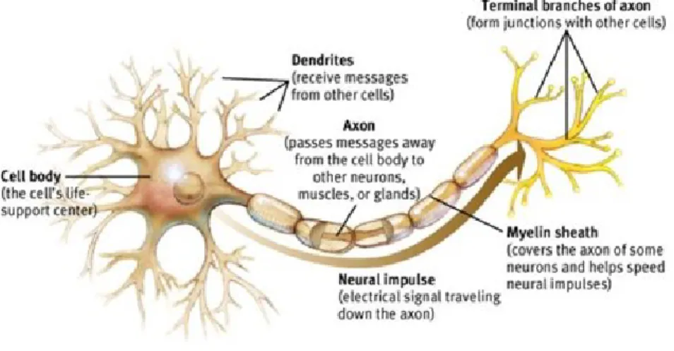
The nervous system is composed of all the nerve cells present in our body. The nervous system receives information from our sensory organs, processes the information, prompts reactions and controls the metabolic processes. The nerve cells are made up a cell body, containing the nucleus, and several extensions, which are two types: (i) dendrites, (ii) axons (Figure 2.1). The dendrites receive signals and transfer it to the cell body, while the axons take signals away from it.

(15)

Figure 2.1: Neuron.

A neuron is composed of a cell body, dendrites and axon surrounded by myelin. This figure was extracted from http://www.appsychology.com/Book/Biological/neuroscience.htm

The nervous system is made up of two parts: (i) the CNS and (ii) the Peripheral Nervous System (PNS). The CNS interacts with the rest of the body through the PNS, which lies outside of the brain and spinal cord and is connected with the rest of the organism. In the PNS, axons or nerve fibbers conduct information from and to the CNS. The CNS incorporates sensory or motor information, coming from the whole organism and regulates the physiological activity. For instances, it controls the breathing, heart rate, hormonal secretion and body temperature. It harmonizes and organizes our thoughts, emotions, desires, movements and memories.

The CNS is composed of the association of the brain and the spinal cord. Although brain is commonly considered as the most fascinating part of the human body, we will try, in this thesis, to put the light on some attractive aspects of the spinal cord.

2.1.2 Spinal cord tracts

The spinal cord is the main bridge between the brain and the rest of the body, connected to the brain through the brain stem. Motor instructions from the brain transit from the brain through the spine to the muscles (descending tracts on Figure 2.2). Sensory information travel from sensory tissues through the cord towards the brain (ascending tracts on Figure 2.2). The spinal cord also controls some reflexive responses and hosts neurons associated with key functions such as locomotion (Rossignol, 2006). The spinal cord nerves can indeed coordinate walking muscles independently of brain activity.

(16)

Figure 2.2: Spinal cord tracts, ascending (sensory) and descending (motor).

Each tract or column is associated with functions indicated into brackets. Figure extracted from

https://commons.wikimedia.org/wiki/File:Spinal_cord_tracts_-_English.svg. P: Posterior, A: Anterior, L: Left, R: Right.

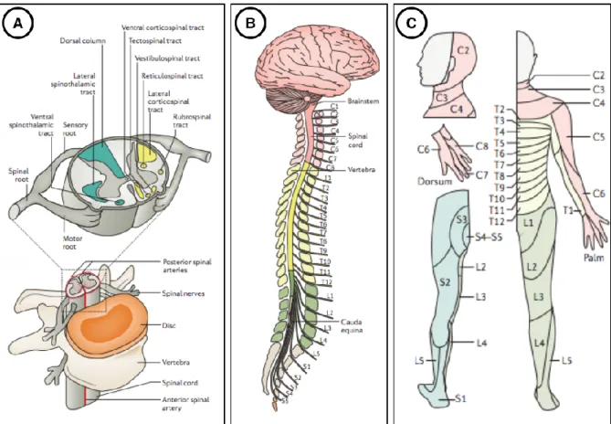
The spinal cord tissue is organized into grey and white matter. Grey matter contains the cell bodies of the neurons, while white matter contains the axons. More precisely, white matter is composed of bundles of axons, transmitting sensory or motor information, belonging either to ascending or descending tracts (Lévy et al., 2015). The white matter can be subdivided into 3 columns: (i) dorsal column (DC), (ii) lateral funiculus (LF), (iii) ventral funiculus (VF), each of them having a very specific role. For instance, DC transmit sensory signal of the touch perception to the somatosensory cortex. Regarding the grey matter and its butterfly-shape, the front “wings’’ (named horns) host motor nerve cells, while the back horns contain sensory nerve cells (see Figure 2.3). As a result, the spatial localization of spinal cord damages is highly associated with the functional impairment, since each spinal pathway has a particular function in the CNS.

(17)

Figure 2.3: Spinal root.

Figure showing the motor nerves (red) entering in the grey matter spinal cord through the ventral root, while sensory nerve transit from the body to the spinal cord through the dorsal root. Figure extracted from http://www.newhealthadvisor.com/Spinal-Cord-Cross-Section.html. P: Posterior,

A: Anterior, L: Left, R: Right.

2.1.3 Spinal canal

The spinal cord is surrounded by a layer of cerebrospinal fluid (CSF) and then protected by the vertebral column. The vertebral discs cushion the vertebral bodies and allow flexibility to the spinal cord (see Figure 2.4 A). The human vertebral column is commonly divided between cervical (7 levels), thoracic (12), lumbar (5) and sacral (5) sections (see Figure 2.4 B). Each region of the spinal cord innervates a particular group of organ, muscle or skin (see Figure 2.4 C). Spinal nerve roots come in the spinal cord either through the sensory or dorsal root to convey sensory information to the CNS, or through the motor or ventral root to transmit motor information to the periphery. Consequently, a damage to the spinal cord could result in a functional impairment below the level of the injury.

(18)

Figure 2.4: Anatomy of the spinal cord.

(A) The spinal cord is made up of grey and white matter. The white matter is subdivided into ascending (green) and descending (yellow) tracts. Spinal nerve roots come in the spinal cord through the sensory, dorsal, ventral or motor roots to transmit motor or sensory information. The vertebral column, mainly composed of discs and vertebral bodies, as well as a protective layer of cerebrospinal fluid protect the spinal cord. (B) The vertebral column is segmented into 7 cervical

(red), 12 thoracic (yellow), 5 lumbar (green) and 5 sacral (grey) vertebrae. Each region of the spinal cord innervates a particular region of the skin (C). Figure adapted from (Ahuja et al.,

2017).

2.1.4 Spinal cord morphometry

Spinal cord has a tubular and ellipsoidal shape, with small dimensions, which vary depending on the vertebral level. Indeed, the mean cross-sectional area of the cervical cord is about 91mm2, compared to 68mm2 for the lumbar cord (Fradet et al., 2014). For adult humans, the

spinal cord has an average length of 45cm (Goto and Otsuka, 1997). Spinal cord curvature follows the vertebral column and differs according to the subject and its position. In particular, a

(19)

significant enlargement of the spinal cord is observed between C4 and C5 (“cervical enlargement”) vertebral levels, as well as between T12 and L1 (“lumbar enlargement”), due to expanded neural input and output to the upper and lower limbs respectively.

(20)

2.2 Spinal cord magnetic resonance imaging

MRI is among the recommended methods to assess spinal cord damages due to its non-invasiveness and sensitivity to parenchymal tissue. In particular, non-invasive imaging methods are essential to image the spinal cord since the surrounding structures make the cord inaccessible for human in-vivo research. Besides of this, the surrounding structures combined with the anatomical configuration of the spinal cord induce important challenges for MR imaging. In this section, we discuss important data features (sub-section 2.2.1) and main challenges of the spinal cord MR imaging (sub-section 2.2.2).

2.2.1 Data features

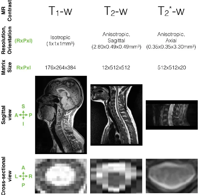
A main challenge of this project was to face the large heterogeneity of data features commonly exhibited by a multi-center dataset, such as the resolution, the field of view, orientation, and the MR contrast. Figure 2.5 depicts some heterogeneous spinal cord MRI samples.

(21)

Figure 2.5: Samples of spinal MRI data.

Samples differ in terms of MR contrast, resolution, orientation, matrix size, field of view. The heterogeneity of these features are visible on the sagittal and cross-sectional view. Note that the spinal cords do not have the same dimensions on the cross-sectional view since they are not from

the same vertebral level. P: Posterior, A: Anterior, L: Left, R: Right, I: Inferior, S: Superior. RxPxI: Right-to-Left x Posterior-to-Anterior x Inferior-to-Superior.

2.2.1.1 Resolution and field of view

In MRI, spatial resolution is the size of the voxels in the 3D acquired image. The resolution can be anisotropic (i.e. 2D acquisition) or isotropic (i.e. 3D acquisition) and depends

(22)

on the matrix size, the field-of-view (FOV), and the slice thickness (see second row of Figure 2.5). The matrix size is defined by (i) the number of frequency encoding steps in one direction, (ii) the number of phase encoding steps in the other direction of the image plane. The FOV determines the amount of coverage over which an MR image is acquired (Fourier space, k-space) or displayed (spatial space). The slice thickness is the voxel depth and is related to the maximum strength of the z-gradient coils and time restraints limiting the number of slices available. Typical resolution used in clinical routine is about 1x1 mm2 in the image plane, and a slice thickness

between 1 and 3 mm. 2.2.1.2 Orientation

Axial scans place the highest spatial resolution in the cross-sectional plane (see last row of Figure 2.5), favouring the spinal cord plan where the anatomy is more varied. However, the main drawback of axial scans is that they usually span a relative small Superior-to-Inferior view (see last column of Figure 2.5) since it is time-consuming to acquire a large number of slices.

Sagittal scans however have a worst resolution in the Left-to-Right direction but are valuable considering the small dimensions of the cord and its relative low curvature in this direction. These images allow to cover large Superior-to-Inferior view but suffer from partial volume effect (PVE) in the cross-sectional plane. Note that the partial volume effect is when several structures may contribute to the signal of the border voxels (see Figure 2.6). In particular, the PVE is even more important when the image slice is not orthogonal to the spinal cord axis. As a result, cross-sectional area measures, such as used for atrophy quantification, is then not recommended on sagittal scans.

(23)

Figure 2.6: Partial volume effect in the cross-sectional plane.

The partial volume effect is when several tissue may contribute to the voxel value. For instance, both white matter and cerebrospinal fluid signals contribute to the value in voxel circled in red.

Figure courtesy from Simon Lévy. 2.2.1.3 MR contrast

For this project, conventional MRI was used while new neuroimaging approaches also exist (e.g. diffusion tensor imaging, and functional MRI). Although the acquisition sequences vary largely across centers, we grouped our data in three datasets (see first row of Figure 2.5):

 “T1-weighted”: dark CSF / light cord, example of sequence

 “T2-weighted”: light CSF / dark cord / grey matter not visible

 “T2*-weighted”: light CSF / dark cord / grey matter visible

2.2.2 Acquisition challenges

The challenges are mainly of 3 types: (i) small cord dimensions in the cross-sectional plane, (ii) physiological motion, (iii) spatial inhomogeneous magnetic field environment.

Compared to other anatomical structures commonly imaged with MRI, like brain or heart, the spinal cord is difficult to image because of its small physical dimensions. Indeed, a typical in-plane spatial resolution of 1x1mm2 does not allow to depict small anatomical details of the spinal

cord (see last row Figure 2.5).

The spinal cord is surrounded by the CSF which flows, non-uniformly, back and forth in the Superior-Inferior direction induced by the heart beat (Matsuzaki et al., 1996). The CSF flow prompts the spinal cord movement inside the spinal canal, which hinder the spinal cord MR

(24)

imaging. It could cause areas of hyperintensity or signal voids. Furthermore, physiological motion induced by respiration, posture or periodic movements (e.g. heart) can make the spinal cord slightly move and causes image artifacts. Axial scans are less prone to motion artifacts (e.g. heart, lungs) thanks to the possibility to use a phase-encoding in the right/left direction.

To acquire MR images in the spinal cord is also challenged by the inhomogeneous magnetic field in this region. Different susceptibilities in the vertebrae, the intervertebral discs and the air-filled lung may produce signal loss and geometric distortions (Verma and Cohen-Adad, 2014). Axial scans are less prone to these artefacts than sagittal scans since there is less field variation across the slice thickness.

However, during the last decades, significant improvements were achieved, both in pulse sequences and hardware, in mitigating these issues (Stroman et al., 2014; Ryan Topfer et al., 2018), opening new perspectives for the spinal cord analysis.

(25)

2.3 Spinal cord damage

Spinal cord damage might cause partial or complete loss of the sensory or motor functions, that could lead to different degree of paralysis. They could result from trauma or neurodegenerative diseases. In this section, we will briefly present two diseases, the MS (subsection 2.3.1) and the ALS (subsection 2.3.2), and how they affect the spinal cord tissue.

2.3.1 Multiple sclerosis

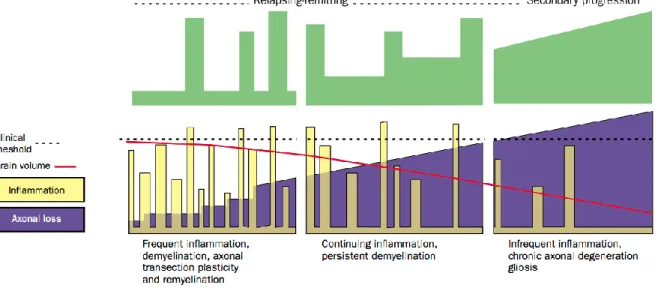
MS is a chronic, inflammatory and demyelinating disease of the CNS. Involved by the inflammation, the myelin degeneration impairs the communication ability of the impacted areas, resulting in physical, mental or psychiatric problems. However, the disease progression (i.e. inflammation events, axonal loss and brain atrophy) are not uniform across patients. Indeed, most of the time, the inflammation disappears and reparation mechanisms (called “remyelination”) could recover the myelin. Nevertheless, the inflammation and demyelination could be too high compared to the remyelination mechanism in some instances, leading to non-reversible connectivity (Compston and Coles, 2002). Depending on the disease progression over time, phenotypes of MS are defined (see Figure 2.7):

 Clinically Isolated Syndrome (CIS) patients, refers to a first episode of neurologic symptoms, caused by inflammation or demyelination.

 Relapsing Remitting MS (RRMS) patients (~85%) alternate over time between “spikes” of disability and (partial or full) recovery. Secondary Progressive MS (SPMS) patients present a constant and non-reversible progression of disability. SPMS follows an initial relapsing-remitting course.

 Primary Progressive MS (SPMS) patients (~15%) are characterized by a progression of the disability without early relapses or remissions. PPMS can be further characterized at different points in time as either active or not active, as well as with progression or without progression.

Note that we called disease progression when there is evidence of disease worsening over time ; and relapse an attack of new or increasing neurologic symptoms.

(26)

Figure 2.7: Course of the Multiple Sclerosis over time.

Cource of Multiple Scleoris over time (Compston and Coles, 2002), in terms of disability (green), inflammation (yellow), axonal loss (violet) and brain atrophy (red). The progression differs for

relapsing-remitting (left) or secondary progressive (right) MS patients.

Compston et al. et al. stated that MRI presents focal or confluent abnormalities in white matter in more than 95% of patients (Compston and Coles, 2002). Demyelination occurs in plaques with various sizes and shapes, in both brain and spinal cord. Figure 2.7 depicts some spinal cord lesions, with either a focal or diffuse appearance. The McDonald diagnostic criteria include the number and size of lesion in the brain and spinal cord detected with MRI (Polman et al., 2011). Briefly, the 2010 McDonald diagnostic criteria can be sum up as follows:

 Dissemination in space: At least one T2 lesion in two of the following areas: spinal cord,

periventricular area, juxtacortical area and infratentorial area

 Dissemination in time: A new T2 and/or gadolinium-enhancing lesion(s) on follow-up MRI as compared with a baseline scan, without regard of the timing of the baseline MRI

(27)

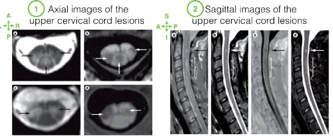
Figure 2.8: Axial and Sagittal views of cervical cord with lesions.

Axial (1) and Sagittal (2) images of the cervical cord. Arrows indicate focal lesions, visible on hyperintense (e.g. 1.a, 2.b) or hypointense abnormalities (e.g. 1.b, 2.c). Note that the lesions extent to grey matter on 1.c and 1.d axial images. Images were acquired with different sequences:

fast-field echo (1.a and 1.c), phase-sensitive inversion recovery (1.c, 1.d and 2.c), proton-density weighted (2.a), T2-weighted (2.b) and short tau inversion recovery (2.d). Note that lesion detectability differs a lot across images. For instance, the diffuse abnormality (indicated by bracket) is clearly visible on (2.a) while the focal lesion is especially clear on (2.b,c,d). Figure

adapted from (Kearney et al., 2015b).

In 1950, Fog observed a lesion predominance in the posterior and lateral white matter (Fog, 1950). In the last two decades, the lesion involvement in the grey matter has been shown, either through a grey-white matter extension, either confined in the grey matter (Bot et al., 2004; Lycklama et al., 2003). As explained in the section 2.1.2, the location of the white-matter lesions is correlated with their clinical impact (see Figure 2.2). However, the effects of grey-matter lesions are still not well understood (Kearney et al., 2013).

SC axonal loss can be vast in MS patients since Lovas et al. showed that axonal density can be reduced by 65% (Lovas et al., 2000). Spinal cord atrophy measured on MRI data has been shown to be a reliable biomarker to monitor the neurodegenerative process in MS patients (Bakshi et al., 2005). SC atrophy may be focal, around a lesion, or extended to a larger portion (Bastianello et al., 2000). It is however important to note that SC atrophy is a nonspecific measure of tissue injury since it includes axonal destruction, demyelination, and other tissue

(28)

degeneration (Bot et al., 2004). SC atrophy demonstrated moderate-to-strong correlation with disability in cross-sectional and longitudinal studies (Kearney et al., 2015a, 2014; Losseff et al., 1996; Stevenson et al., 1998). When comparing phenotypes populations, spinal cord atrophy was more pronounced in progressive forms of MS (i.e. SPMS and PPMS patients), and especially greatest in SPMS patient (Losseff et al., 1996). Among progressive forms, the rates of atrophy in the brain and in the spinal cord are different in PPMS patients, suggesting differences in the underlying pathological processes between the brain and the spinal cord (Ingle et al., 2003). Finally, cord atrophy holds an important diagnosis value since it is present already in the earliest stages of the disease (Biberacher et al., 2015).

2.3.2 Amyotrophic lateral sclerosis

ALS is a progressive and highly heterogeneous neurodegenerative disease, mainly affecting the motor neurons in the cerebral cortex, brainstem and spinal cord. The degeneration of the lower and upper motor neurons results in muscle weakness, atrophy or clumsiness. The muscle size decrease leads to loss of autonomy, speaking or breathing impairment, which can lead to death. ALS is characterized by a short survival rate (median survival from onset: 23–52 months) (Blumenfeld, n.d.; Brooks, 1996). Although implication of genetics has been recognized (Renton et al., 2014), the knowledge of the mechanisms leading to this disease are still insufficient and the cause is not known for most cases. At present, this disease remains incurable and there is a lack of proper treatment.

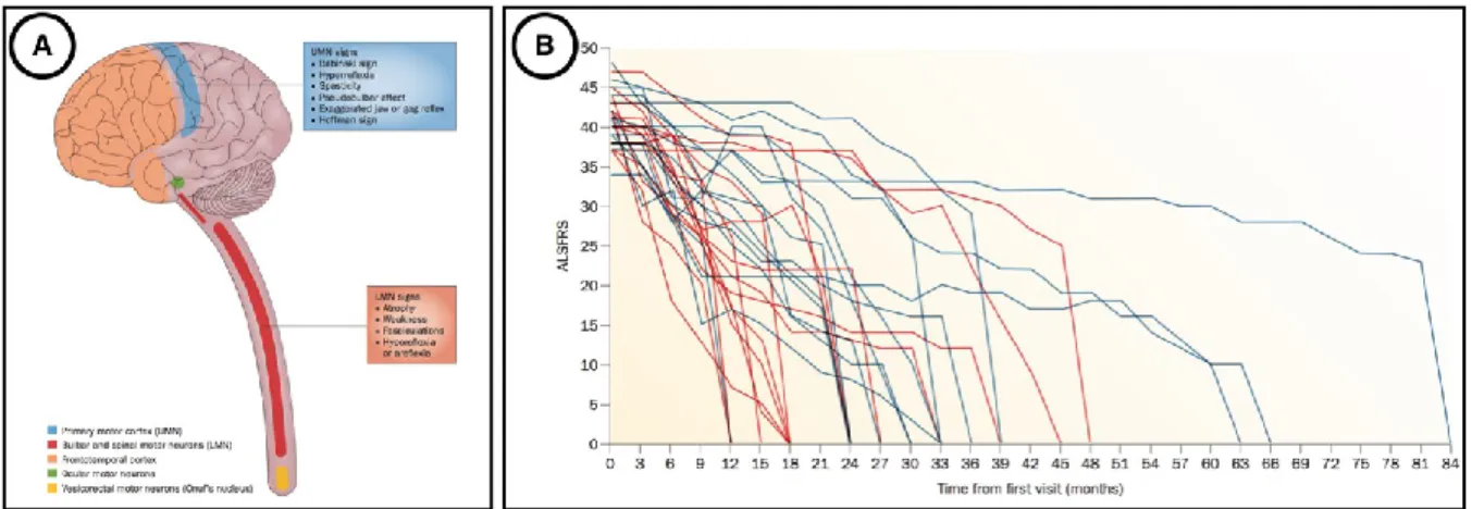
The large heterogeneity of clinical features present in the early course of ALS hampers an absolute diagnosis (Brooks, 1994). Briefly, the ALS diagnosis focuses on the presence of signs of upper and lower motor neuron dysfunction within the same body segments. In most cases, ALS onset is located in spinal or bulbar regions (see Figure 2.9 A). However, ALS clinical presentation and progression are highly heterogeneous among patients (see Figure 2.9 B). The assessment of the timing and the monitoring method of a patient account for an important reason for the clinical variability (Swinnen and Robberecht, 2014). The development of robust biomarkers could better categorize clinical phenotype, improve prognosis, identify the true biologic effects of drug testing in clinical trials, and more generally promote a better understanding of the physiopathology processes of the disease (Turner and Verstraete, 2015). In particular, biomarkers of the spinal cord can potentially provide a relevant measure of the

(29)

degeneration of lower motor neurons (Cohen-Adad et al., 2013; El Mendili et al., 2014; Turner and Benatar, 2015). El Mendili et al. established that cord atrophy measured with MRI was a valuable biomarker of disease progression, improving prediction of the arm-revised ALS Functional Rating Scale (ALSFRS-R) subscore at 1 year (El Mendili et al., 2014). Cohen-Adad et al. showed that local spinal cord atrophy was correlated with deficiency in the corresponding muscle territory (e.g. C4 level for deltoid and C7 level for hand muscles). The idea behind it is that detecting local SC atrophy on MRI data, corresponding to specifically altered muscles, could be a reliable non-invasive quantification of lower motor neuron degeneration.

Figure 2.9: Phenotypic variability of ALS patients.

(A) shows the preferential locations of neuronal areas impaired by ALS disease. The main involved regions are the upper motor neurons (UMN) in the motor cortex (blue) and the lower motor neurons (LMN) in bulbar or spinal regions (red). (B) illustrates the variability of disease progression scored by the ALSFRS (ALS Functional Rating Scale), from the diagnostic onset to

death. The 30 patients involved here had either a bulbar onset (red), either a spinal onset (blue). Figure adapted from (Swinnen and Robberecht, 2014).

(30)

2.4 Automatic segmentation of the spinal cord on MRI data

The automatic segmentation and/or detection of the spinal cord on MRI data is a necessary first step towards the segmentation of MS lesions within it. Moreover, the characterization and localization of the spinal cord impairments is clinically relevant and holds an important prognostic value for functional recovery. In this section, we present a literature review of the preprocessing methods (sub-section 2.4.1) frequently used before performing an automatic detection (sub-section 2.4.2) or segmentation (sub-section 2.4.3) of the spinal cord. A brief review of automatic segmentation methods used in the brain for MS lesions is also introduced (sub-section 2.4.4).

2.4.1 Preprocessing

Most automatic segmentation frameworks rely on a first stage of pre-processing for data preparation and/or enhancement. Overall, these preprocessing steps have to compromise the robustness across multi-center datasets, flexibility in terms of number of tunable parameters, computation time and efficiency to facilitate the subsequent segmentation.

2.4.1.1 Field of view cropping

FOV cropping or region of interest assumptions are required by some algorithms to guarantee the spinal cord to be approximately centered in the image (Koh et al., 2011, 2010; Perone et al., 2017). This cropping could certainly help the spinal cord detection and/or the class imbalance by reducing the background in the investigated volume to segment. However, an automatic cropping is not always feasible without prior knowledge or detection, especially in multi-center datasets where the FOV can substantially vary across centers. On sagittal scans commonly presenting a small Right-to-Left coverage, automatic cropping could suffer from an incorrect position of the patient in the scanner. Finally, because of the spinal cord curvature, the cord frequently spans a large portion of the Anterior-to-Posterior axis.

To overcome this problem, an automatic spinal cord detection module, prior to the segmentation, could be of interest, as done by De Leener et al. (De Leener et al., 2014).

(31)

2.4.1.2 Image denoising

Noise in an MRI image is produced by the static fluctuation of signal intensity, mainly caused by (i) the molecular movement of charged particles in the subject body, (ii) electrical resistance from some hardware components (e.g. receiver coils). Denoising is an important step to enhance image quality. However, a perilous issue in the restoration of the image is the dilemma of noise removal while preserving the relevant image information (Buades et al., 2005).

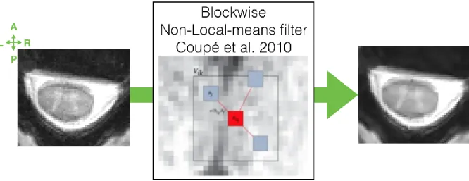
One of the most used method of denoising for 3D MRI data is certainly the one proposed by Coupe et al. (Coupe et al., 2008) based on block-wise non-local-means filters. Briefly, the non-local-means filter exploits the redundancy property of MRI images to remove the noise. Most of the previously proposed denoising approaches restore the intensity of each voxel by averaging the intensities of its neighboring voxels. In this approach, the weight involving voxels in the average is based on the intensity similarity between their neighborhoods (blue block in Figure 2.10) and the neighborhood of the voxel under study (red block in Figure 2.10). This method was confirmed to efficiently remove the noise while preserving the edges. Figure 2.10 depicts its utilization on spinal cord data, where it could be relevant for performing automatic grey matter segmentation since it increases the grey/white matter contrast.

Figure 2.10: Block-wise Non-Local-means filter.

The Block-wise Non-Local-means filter (Coupe et al., 2008) is applied to the left image, and results in the right one. This algorithm is illustrated: the restored value of the block of voxels Bik

results from the weighted average of all the Bj blocks within the volume Vik.

A critical review assessed the effects of denoising techniques (Gaussian filter, anisotropic diffusion, wavelet, and non-local-mean) on MRI brain tumor segmentation (Diaz et al., 2011).

(32)

Although the image noise was lessened by using denoising algorithms, they could introduce undesirable artifacts, harmful for the segmentation task. However, they recognized non-local-means algorithm as the most appropriated denoising technique for brain tumor segmentation. 2.4.1.3 Image normalization

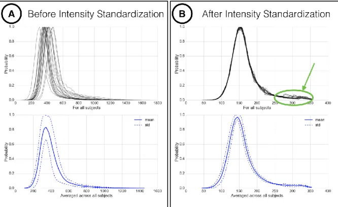
One of the main difficulties with non-quantitative MR scans is that intensity values do not have a fixed meaning, not even for data acquired with the same protocol or with the same scanner, for the same imaged organ...etc (see Figure 2.11 A). Therefore, a direct comparison of intensities between two MR scans is not feasible since the intensities are not standardized. Image normalization is a process of mapping similar tissue types to closer intensity values (see Figure 2.11 B). In particular, intensity normalization has played important role for a large number of parametric supervised automatic image segmentation methods, which rely on the intensity distributions on a standardized intensity range.

Nyúl et al. proposed a method including (i) a training stage to learn a set of intensity landmarks, based on the histogram percentiles and (ii) a transformation stage to map the original intensities between two landmarks, into the corresponding learned landmarks using linear transformations (Nyúl and Udupa, 1999). Improvements of this initial version were then proposed, especially using deciles piece-wise linear mapping (Nyúl et al., 2000). This method remains widely used as pre-processing step for MRI data analysis/segmentation (Koch et al., 2017; Pereira et al., 2016; Xiao et al., 2015) and was validated on MS MRI data (Shah et al., 2011). Pereira et al. showed that CNN-based classifiers also improve after Nyúl normalization (mean gain of 4.6% in their evaluation metrics), at least in the context of brain tumor segmentation on MRI data (Pereira et al., 2016). Recently, other methods were proposed (Roy et al., 2013; Sun et al., 2015), arguing that landmark-based methods could suffer from the difficulty of learning reliable landmarks and from time-consuming hyper-parameter tuning.

(33)

Figure 2.11: Intensity normalization proposed by Nyúl et al.

Illustration of the intensity normalization proposed by Nyúl et al. (Nyúl and Udupa, 1999) on 20 spinal cord MRI volumes of MS patients, acquired in the same center with the same sequence. The top row histograms represent the intensity distribution computed within the spinal cord of each patient, while the bottom row shows the mean (and standard deviation) histograms across patients. Spinal cord intensities across subjects have closer values after standardization (B). Moreover, some outliers (circled in green) are clearly more visible than before standardization

(A), which could help the detectability of MS lesions. 2.4.1.4 Bias field correction

In order to compensate for the effect of magnetic field inhomogeneities during image acquisition, bias field corrections methods are commonly employed (Vovk et al., 2007). Bias field correction is notably relevant for spinal cord images where intensity variation induced by the B1+ and B1- inhomogeneities are frequent (see section 2.2.2). N3 and N4 algorithms are

among the most prevalent techniques used in MRI (Sled et al., 1998; Tustison et al., 2010). Briefly, these methods perform a non-parametric, non-uniform, intensity normalization by estimating the multiplicative bias field among true tissue intensities, in order to correct it using B-spline least-squares fitting. Although N4 correction provides satisfying results (see Figure 2.12),

(34)

to find appropriated hyper-parameters is difficult and time-consuming. Moreover, issues are often noticed at the extreme slices of the data since they are related to the extreme points of the regularized mesh.

Figure 2.12:Bias field correction using N4ITK algorithm.

Comparison of a sagittal view of a spinal cord MRI data before (A) and after (B) bias field correction using N4ITK algorithm (Tustison et al., 2010). The field inhomogeneity (circled in green) has been partially corrected since the variation of the mean intensity per slice (along the

Superior-to-Inferior axis) has been reduced.

2.4.2 Automatic detection of the spinal cord

2.4.2.1 Rational and challenges

Detecting the spinal cord position within MRI volumes is an essential step for automating quantitative analysis pipelines. For instance, this step plays a key role in recent published pipelines such as spinal cord (De Leener et al., 2014; Horsfield et al., 2010) and grey matter (Dupont et al., 2017; Prados et al., 2017) segmentations, template registration (De Leener et al., 2018; Stroman et al., 2008) and B0 susceptibility-related distortion correction (R. Topfer et al., 2018; Vannesjo et al., 2017).

While detecting the spinal cord might appear as an elementary computer vision task, it is much more challenging to achieve it accurately and robustly across a large variety of spinal cord shapes (see Figure 2.13), craniocaudal vertebral length, pathologies (e.g. compressed or

(35)

atrophied cords or hyperintense lesion areas), image FOV, image resolution and orientation, types of contrast and image artifacts (e.g. susceptibility, motion, chemical shift, ghosting, blurring, Gibbs). In the particular case of spinal cord segmentation, a recent review paper identified 20 recently-published spinal cord segmentation methods requiring manual intervention for initialization (De Leener et al., 2016). Especially, a number of these methods require the user to manually identify specific anatomic landmarks within the spinal cord. Hence, these methods could potentially be made fully automatic if initialized with a robust automated spinal cord centerline detection module.

Figure 2.13:Samples of spinal cord MRI data in the cross-sectional plane.

This figure shows a large heterogeneity in terms of cord appearance depending on the MR contrast (T1-, T2*-, T2-weighted), the vertebral levels (yellow, C: cervical, T: thoracic, L: lumbar,

PMJ: pontomedullary junction), the resolution in the cross-sectional plane, the pathologies (compression, lesion). DCM: Degenerative cervical myelopathy, HC: healthy control, MS:

(36)

2.4.2.2 Related works

A common approach to automatically detect the spinal cord is to target the characteristic ellipsoid shape of the spinal cord in the cross-sectional plane. De Leener et al. proposed to detect ellipsoid shape resorting to the Hough transform combined with vesselness filtering (De Leener et al., 2014). While this approach has shown good performances, ellipsoid pattern detection is challenged by severe cord atrophy with poor CSF/SC contrast or by the important partial volume effect in the cross-sectional plane of sagittal scans. Koh et al. presented an approach based on gradient vector flow field to find the candidate structures combined with a connected component analysis (Koh et al., 2010). However, this method assumes a specific region of interest, and is designed to only work on 2D images, sagittal view, T2-weighted MR contrast.

Carbonell-Caballero et al. employed a template-based method by registering a cord pattern to the subjects’ scan using cross-correlation (Carbonell-Caballero et al., 2006). Although this method was extensively validated, a major drawback is its restriction to 2D T2-w axial slices of the cervical spine. Chen et al. resorted to a deformable atlas associated with topology constraints, while making no assumptions on image resolution or FOV (Chen et al., 2013). In particular, topology constraints (classification atlas of the spinal cord, CSF and background) are used to ensure the integrity of the detected spinal cord.

2.4.3 Automatic segmentation of the spinal cord

2.4.3.1 Rational

Spinal cord segmentation is a mandatory step towards automated interpretation of morphometric and multi-parametric spinal cord MRI data. For instance, we present below 2 recent studies using the spinal cord segmentation for 2 distinct applications:

 Hori et al. evaluated the sensibility of quantitative metrics as potential clinical biomarkers for degenerative cervical myelopathy patients (Hori et al., 2018). These metrics were computed from the atlas-based regions combining information from diffusion and magnetization transfer weighted images. To do so, they used spinal cord segmentation for co-registrating all available data to a common coordinate space, allowing atlas-based quantitative multi-parametric analyses.

 Ventura et al. aimed at characterizing the atrophy process of neuromyelitis optica spectrum disorder in light of the disease evolution (Ventura et al., 2016). The cross-sectional area of the

(37)

spinal cord, obtained from its segmentation, provided them a quantitative assessment of the cord atrophy.

Automatic segmentation methods have great potential for studies involving a large number of subjects or for longitudinal analyses. Indeed, manual segmentation is highly time-consuming and suffers from inter- and intra-variability.

2.4.3.2 Challenges

In this section, we summarized the main challenges of the automatic spinal cord segmentation on MRI data, even if most of them were already mentioned in the previous sections.

Although the spinal cord shape is roughly similar to an ellipsoid in the cross-sectional plane, it is not consistent across subjects and even within a subject. Papinutto et al. showed that age and gender had a significant impact on the total cross-sectional area: women having smaller values than men, elderly smaller values than younger (Papinutto et al., 2015). Within a subject, the ratio of the first and second radii can change along the Superior-to-Inferior axis (see Figure 2.13).

In general, the spinal cord exhibits a substantial intensity gradient with the surrounding CSF, which could be highly useful for the automation of the spinal cord delineation. However, this might be challenged by: (i) the natural cord curvature leading to portions where the spinal cord directly touches the spinal canal, (ii) the partial volume effects (cf Figure 2.6), (iii) pathological hyperintense signal (e.g. MS lesions) or cord deformation (e.g. trauma, ALS, SCI…), as illustrated in Figure 2.13.

Finally, the automatic spinal cord segmentation can be hindered by MR artefacts, as detailed in section 2.2.2, such as (i) CSF flow artifacts resulting in areas of hyperintensity or signal voids, (ii) Gibbs artifacts leading to ringing lines parallel to large intensity gradients in the image, (iii) static noise, (iv) signal loss due to B1- inhomogeneities, (v) contrast alterations due to B1+ inhomogeneities.

(38)

2.4.3.3 Related works

In 2014, De Leener et al. made a review of the existing semi-automatic or automatic methods for spinal cord segmentation on MRI data (De Leener et al., 2016). The authors classified spinal cord segmentation methods in the following categories:

 Intensity-based, examples: feature extraction (e.g. Hough transform), thresholding (e.g. Otsu), edge detection (e.g. Kalman)

 Surface-based, examples: active-contours (B-spline), deformable models (tubular surface propagation)

 Image-based, examples: template/atlas, clustering/classifiers

Among the 26 methods listed in this review paper, only 6 were fully automatized (Koh et al. 2010; De Leener et al. 2014; Carbonell-Caballero et al. 2006; Chen et al. 2013; Pezold et al. 2015; Tang et al. 2013). In most of the 20 semi-automatic methods, the required manual intervention consists in adding some landmarks within the spinal cord (as explained in the section 2.4.2.1). Regarding the 6 fully automatic methods, some assumptions or limitations hamper their utilization in clinical studies:

 Region of interest assumption, which limits its utilization for multi-center studies where the field of view is not necessary common across centers

 MR contrast restriction, which limits its utilization for studies with several modalities  2D data restriction, while most of MRI data are 3D

 Lack of validation on pathological cases, which are frequently substantially more challenging than healthy subjects (e.g. compressed cord, hyperintense lesions)

 Lack of validation across a variety of data features, which is a required validation step before considering its utilization in multi-center studies

 Repeatability limitation, since most of the methods are not publicly available, which hinder its wide dissemination through research groups and clinical routine

Among the previously published methods, PropSeg (De Leener et al., 2014) received sustained attention from the community. Figure 2.14 presents the gist of this automatic method.

(39)

Figure 2.14: PropSeg’ method for automatically segmenting the spinal cord.

The segmentation workflow begins with a spinal cord detection module (1): an elliptical Hough transform is applied around the median cross-sectional plane to find potential spinal cord position, then corrected thanks to a neighborhood analysis and a discriminant validation. The spinal cord segmentation is then performed (2) by propagation of a deformable model composed

of triangular meshes (Mi). Figure adapted from (De Leener et al., 2014).

PropSeg has many advantages, which might be valuable to mention. The authors devised a model specifically designed for the spinal cord, based on anatomical priors. For instance, the method takes advantage of the tubular shape of the spinal cord thanks to a deformable model combined with a global deformation, which guarantee the continuity and integrity of the output segmentation. Moreover, PropSeg is robust to different MR contrast (T1-, T2, T2*-weighted) and

makes no assumption about field of view, image resolution or orientation. This is an unsupervised method, which means there is no need for manual annotation to train a model. In case of segmentation failure with the default parameters, the model can be adjusted (e.g. radius of the SC, conditions on the deformation) in order to refine the segmentation. In volumes that include brain sections, the method accurately separates brain and spine regions using a criterion on the mesh radius to stop its propagation. Furthermore, the method is fast (less than 1 minute on a typical T2-weighted scan) and has been validated against MS patients with atrophy (Yiannakas

(40)

software, the Spinal Cord Toolbox (De Leener et al., 2017), and further improved thanks to a massive feedback received from the community (De Leener et al., 2015).

However, it is important to note some drawbacks of this existing solution. First, the Hough transform can be challenged in instances of deformed cords, which might be critical since the segmentation performance highly depends on the detection status. As user of this method, I also noticed that (i) under-segmentation is quite frequent for T2*-weighted images when the

contrast CSF/cord is low, (ii) the segmentation tends to leak out of the cord in instances of severe cord compression.

2.4.4 Automatic segmentation of MS lesions

2.4.4.1 Rational

Several studies show evidence of the importance of SC lesions for diagnosis and prognosis of MS at clinical presentation (Arrambide et al., 2018; Sombekke et al., 2013; Thorpe et al., 1996). Arrambide et al. stated that MR scans to image spinal lesions are valuable for predicting the disease evolution of CIS patients (Arrambide et al., 2018). Sombekke et al. found that the presence of spinal cord lesions promotes diagnosing MS (Sombekke et al., 2013), in particular in CIS patients who do not fulfill brain MRI criteria but with onset of symptoms originating from the brain.

To illustrate the utilization of MS lesion segmentation in the spinal cord, we have listed below 2 recent studies using it:

 Hua et al. aimed at evaluating the relation between the cervical spinal cord lesions and the presence of thoracic cord lesions (Hua et al., 2015). They determined that the cervical spinal cord lesion involvement could predict the thoracic lesion involvement, independently of the brain involvement or the clinical status. Based on the lesion count, Figure 2.15 (1) presents the spinal cord lesion distribution by vertebral level impacted.

 Valsasina et al. analyzed the spatial distribution of T1-weighted cervical cord lesions in MS

patients (Valsasina et al., 2018). They found that the lesion involvement was greater in the upper than lower cervical level, in the posterior than anterior cord. They also studied correlations between MS spinal cord damages and clinical disability.

(41)

Figure 2.15: Examples of 2 clinical studies using spinal cord MS lesions segmentation. (1) shows the spinal cord lesion distribution depending on the vertebral level (Hua et al., 2015). We observed that the lesional frequency of cervical (C1-C7) spinal levels is higher than thoracic (T1-T12) ones. (2) depicts T1-weighted MS lesion probability maps (Red-Yellow), overlapped by

significant cord atrophy clusters (Blues) when compared to healthy controls, depending of MS phenotype populations (Valsasina et al., 2018).

2.4.4.2 Challenges

The previous subsection illustrated the great interest in segmenting lesions within the spinal cord. To perform an automatic segmentation of lesions is however highly challenging. In addition to the challenges commonly faced when segmenting spinal cord MRI data, some are specific to the lesions. An intensity bias field in the Superior-to-Inferior axis (see Figure 2.12) could lead to a large intensity overlap between lesion and with spinal cord intensities. Moreover, the partial volume effect and the confounding intensities of lesions with normal structure (e.g. grey matter on T2*-weighted images) may mislead the segmentation. While the spinal cord

exhibits most of the time a consistent appearance, lesions are highly heterogeneous in terms of location, size and shape. Finally, lesions are small and sparse objects leading to a very small proportion of lesion voxels compared to the rest of the volume. Figure 2.16 depicts some of these aspects.

(42)

Figure 2.16: Intramedullary MS lesion – Segmentation challenges.

Sample of a spinal cord cross-sectional slice of MRI volume (T2*-weighted contrast). A MS

lesion is visible within the spinal cord (pink arrow). Lesion voxels represents less than 0.01% of the entire volume. The intensity histograms of the spinal cord and lesion voxels are shown: a large overlap between the two tissues. This is especially due to the healthy grey matter exhibiting

similar intensities than lesions. 2.4.4.3 Related works

At the writing time of this section, a thorough search of the relevant literature did not yield available related work. In contrast, automatic segmentation of brain MS lesions was largely investigated in the brain (García-Lorenzo et al., 2013; Lladó et al., 2012). For instance, in 2013, Garcia-Lorenzo et al. identified 47 automatic different methods applied to brain MS lesion segmentation (García-Lorenzo et al., 2013). In this subsection, we will review some recent approaches proposed for brain lesions.

As suggested by two recently-published review papers (García-Lorenzo et al., 2013; Lladó et al., 2012), the methods of automatic MS lesions segmentation on MRI data can be classified between the supervised and unsupervised methods. Supervised methods learn lesions’ characteristics based on manually labeled training data, which are used to optimize a function from inputs to the related labels. Contrary, unsupervised methods learn lesion properties by inferring a function to describe the structure or relationships between the "unlabeled" images.

Unsupervised approaches try to encode the clinical knowledge of MS disease to perform automatic segmentation on each image independently. However, the translation from the expert knowledge to the algorithm code is highly complex, mainly because of the high heterogeneity of