HAL Id: inserm-01304109
https://www.hal.inserm.fr/inserm-01304109
Submitted on 19 Apr 2016
HAL is a multi-disciplinary open access
archive for the deposit and dissemination of
sci-entific research documents, whether they are
pub-lished or not. The documents may come from
teaching and research institutions in France or
abroad, or from public or private research centers.
L’archive ouverte pluridisciplinaire HAL, est
destinée au dépôt et à la diffusion de documents
scientifiques de niveau recherche, publiés ou non,
émanant des établissements d’enseignement et de
recherche français ou étrangers, des laboratoires
publics ou privés.
Automatic graph cut segmentation of multiple sclerosis
lesions
Laurence Catanese, Olivier Commowick, Christian Barillot
To cite this version:
Laurence Catanese, Olivier Commowick, Christian Barillot. Automatic graph cut segmentation of
multiple sclerosis lesions. ISBI Longitudinal Multiple Sclerosis Lesion Segmentation Challenge, Apr
2015, New York, United States. �inserm-01304109�
AUTOMATIC GRAPH CUT SEGMENTATION OF MULTIPLE SCLEROSIS LESIONS
Laurence Catanese
?Olivier Commowick
?Christian Barillot
??
VisAGeS U746 INSERM / INRIA, IRISA UMR CNRS 6074, Rennes, France
ABSTRACT
A fully automated segmentation algorithm for Multiple Scle-rosis (MS) lesions is presented. Our method includes two main steps: the detection of lesions by graph cut initialized with a robust Expectation-Maximization (EM) algorithm and the application of rules to remove false positives. Our algo-rithm will be tested on the ISBI 2015 challenge longitudinal data. For each patient, a unique parameter set is used to run the algorithm.
Index Terms— Graph Cut, Expectation-Maximization, multiple sclerosis, tissue classification
1. INTRODUCTION
Manual and semi-automatic segmentation methods are very time consuming and can show a high variability among man-ual delineations, especially on longitudinal data. To solve this issue, we present a fully automated method for MS le-sions segmentation based on the combination of graph cut and robust EM tissues segmentation using multiple sequences of Magnetic Resonance Imaging (MRI). The algorithm is based on several previous segmentation algorithms. A fully auto-mated method implies that it does not include user interac-tions. Our process is applied to the ISBI 2015 challenge data for longitudinal MS lesion segmentation. Only one parameter set per patient is used. No training steps are involved in the workflow and we do not use the longitudinal information to obtain the segmentation of a given time point.
2. DATA AND PRE-PROCESSING
The challenge dataset includes T1-w, T2-w, PD and FLAIR sequences. The challenge data will not be described further in this paper, more details can be found on the challenge web-site1. In order to reduce the dependency of the segmenta-tion results on pre-processing performance, the data provided for the challenge is already rigidly co-registered in the same space, skull-stripped and the inhomogeneities are corrected. Therefore, in the following the described method will focus only on the MS lesions segmentation itself. Our algorithm re-quires a map of the brain to reduce the region of interest. As
1http://iacl.ece.jhu.edu/MSChallenge
the brain extraction has already been performed, we only add a pre-processing step and threshold the T2-w image to use it as a brain mask.
3. MS LESIONS SEGMENTATION WORKFLOW 3.1. Lesions detection using graph cut
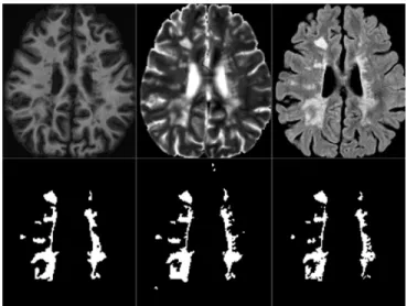
The segmentation algorithm relies on a graph cut previously presented in [1]. This algorithm requires 3 MR sequences. In our workflow, we choose to use T1-w, T2-w and FLAIR sequences and to discard PD as it generally shows less MS lesion contrast than T2-w and FLAIR. An example of seg-mentation result is shown figure 1.
Graph cut principle: The image is represented as a graph where each node is a voxel. Each node is connected to two particular nodes called terminal source and sink which re-spectively represent the object class for MS lesions and the background class for normal appearing brain tissues (NABT). Based on both contour and regional information, the graph cut allows computing an optimal segmentation of the object from a set of seed points. Spatially neighboring nodes are connected by n-links weighted by boundary values that re-flect the similarity of the two considered voxels. The con-tour information contained in the n-links weights is computed using a spectral gradient [1]. The regional term represents how the voxel fits into given models of the object and back-ground. The edges between a node of the image and the termi-nal source and sink nodes are called t-links. Normally these models are estimated using seeds given by the user. Instead, we use an automated version of the graph cut where the ob-ject and background seeds for the initialization are computed from the images. To do so we use a 3-class multivariate Gaus-sian mixture model (GMM), each class representing a tissue of the brain: Cerebrospinal Fluid (CSF), Grey Matter (GM) and White Matter (WM). MS lesions will not be a new class but considered as the outliers of this NABT model.
Seeds computation: The NABT model is estimated us-ing a robust EM algorithm [2] which optimizes a trimmed likelihood in order to be robust to outliers, controlled by the rejection ratio h that represents the portion of voxels that are removed from the estimation. The algorithm then alternates
Fig. 1. Dataset training 02 time point 1: Top, from left to right: T1-w, T2-w and FLAIR. Bottom, from left to right: ground truth 1, ground truth 2 and automatic segmentation.
between the computation of the GMM parameters and the h% outlier voxels. This parameter needs to be high enough to take into account that MS lesions need to be rejected from the model as well as other outliers like veins or skull stripping errors. To process the challenge data, we set h to 20% of the total number of voxels. From the GMM NABT parameters, we then compute a distance of each voxel to each class of the NABT model as a Mahalanobis distance. From this distance, a p-value can be computed, representing the probability not to fit into each of the 3 classes. For each voxel i, we keep the lowest p-value among the three classes, denoted pi. Sinks
represent voxels that are close to the NABT model, therefore they should have a high value when not outliers. The sinks t-links weights Wbiare then computed as:
Wbi = 1 − pi (1)
All voxels that do not fit in the NABT model have a high p-value. To differentiate MS lesions from other outliers (ves-sels,...), we use a priori knowledge: MS lesions are usually hyperintense compared to the WM in T2-w and FLAIR im-ages. Instead of using a clear threshold, we define fuzzy weights between 0 and 1, based respectively on T2-w hyper-intensities (WT 2) and FLAIR hyper-intensities (Wf lair) (see
[1] for more details). We compute the final sources weights Woi by taking the minimum value between the p-value and
the fuzzy weights WT 2and Wf lair:
Woi= AND(pi, WT 2, Wf lair) (2)
3.2. Refinement of the classification
After the detection of candidates lesions, some post-processing steps are performed as false positives may still remain in the
detected outliers. Intensity rules may not be enough to discard false positives, therefore we also use localization information. Considering that MS lesions are typically located in WM, we remove the detected ones that do not sufficiently achieve this condition. Those touching the brain mask border are also eliminated since they are probably false positives due to ves-sels or errors in the skull stripping. Finally, all candidate lesions having a size lower than 3mm3are discarded.
3.3. Contour adjustment
Even if a lesion is correctly detected, it does not mean that the contour of the lesion fits the ground truth since MS lesions do not always have a clear border and differ according to the sequence. This may lead to variability on the lesions load and the consideration of the evolution of lesions. When a lesion occurs, it is generally represented by a cavity that has very clear contours inside the WM mask. Thus we consider the whole cavity as a lesion if at least one voxel overlaps with a lesion voxel on the previously computed segmentation mask. 3.4. Computation time
The algorithm benefices of a multi-threaded implementation. The total computation time to process each time point of the dataset on a laptop with an Intel Core i7 CPU 2.40GHz (8 cores) is approximately 13 minutes.
4. CONCLUSION
We presented a fully automated method for MS lesions seg-mentation using a graph cut initialized with a robust EM, re-moving all the dependencies to human interactions. How-ever, MS lesion segmentation is a complicated task since the definition of MS lesion is not very precise. There is a high variability in the detection of lesions even in between manual delineations of experts (the Dice scores between two ground truth given for the training data vary from 0,59 to 0,88). Some of the MR acquisitions can have a low initial resolution, com-plicating the computation of a good segmentation. Therefore setting rules for the segmentation can be difficult as well as setting the input parameters.
5. REFERENCES
[1] D. Garcia-Lorenzo et al., “Multiple sclerosis lesion seg-mentation using an automatic multimodal graph cuts,” in MICCAI, 2009, vol. 5762 of LNCS, pp. 584–591. [2] D. Garcia-Lorenzo, S. Prima, and Douglas L. Arnold,
“Trimmed-likelihood estimation for focal lesions and tis-sue segmentation in multisequence mri for multiple scle-rosis,” in IEEE Trans. Med. Imag. IEEE, 2011, vol. 30, no. 8, pp. 1455–1467.