Use of artificial neural networks for helicopter load monitoring

(1)

Publisher’s version / Version de l'éditeur:

Proceedings of the 7th DSTO International Conference on Health & Usage Monitoring, 2011-03-03

READ THESE TERMS AND CONDITIONS CAREFULLY BEFORE USING THIS WEBSITE.

https://nrc-publications.canada.ca/eng/copyright

Vous avez des questions? Nous pouvons vous aider. Pour communiquer directement avec un auteur, consultez la

première page de la revue dans laquelle son article a été publié afin de trouver ses coordonnées. Si vous n’arrivez pas à les repérer, communiquez avec nous à PublicationsArchive-ArchivesPublications@nrc-cnrc.gc.ca.

Questions? Contact the NRC Publications Archive team at

PublicationsArchive-ArchivesPublications@nrc-cnrc.gc.ca. If you wish to email the authors directly, please see the first page of the publication for their contact information.

NRC Publications Archive

Archives des publications du CNRC

This publication could be one of several versions: author’s original, accepted manuscript or the publisher’s version. / La version de cette publication peut être l’une des suivantes : la version prépublication de l’auteur, la version acceptée du manuscrit ou la version de l’éditeur.

Access and use of this website and the material on it are subject to the Terms and Conditions set forth at

Use of artificial neural networks for helicopter load monitoring

Liu, Andrew; Cheung, Catherine; Martinez, Marcias

https://publications-cnrc.canada.ca/fra/droits

L’accès à ce site Web et l’utilisation de son contenu sont assujettis aux conditions présentées dans le site LISEZ CES CONDITIONS ATTENTIVEMENT AVANT D’UTILISER CE SITE WEB.

NRC Publications Record / Notice d'Archives des publications de CNRC: https://nrc-publications.canada.ca/eng/view/object/?id=9cd23c4d-7cd1-4568-9407-7c5a74c6331a https://publications-cnrc.canada.ca/fra/voir/objet/?id=9cd23c4d-7cd1-4568-9407-7c5a74c6331a

(2)

AIAC14 Fourteenth Australian International Aerospace Congress

7th DSTO International Conference on Health & Usage Monitoring (HUMS 2011)

This paper has been peer reviewed

Use of Artificial Neural Networks for Helicopter Load

Monitoring

Andrew Liu1, Catherine Cheung1*, Marcias Martinez1 1

Structures and Materials Performance Laboratory, Institute for Aerospace Research, National Research Council Canada, 1200 Montreal Rd, Ottawa, Ontario, Canada K1A 0R6

Abstract

The operational loads experienced by rotary-wing aircraft are more complex than those of fixed-wing aircraft due to the dynamic rotating components operating at high frequencies. As a result of the large number of load cycles produced by the rotating components and the wide load spectrum experienced from a rotary-wing aircraft’s broad range of manoeuvres, the fatigue lives of many components can be affected by even small changes in loads. Ongoing practical load monitoring methods have the potential to improve the accuracy of calculated component retirement times. Direct loads monitoring, however, can be difficult and often-times impractical with high equipment costs and large data storage requirements. This paper explores the potential of utilizing multi-layer artificial neural networks (ANNs) to determine airframe loads at fixed locations from flight state and control system (FSCS) parameters obtained during a Black Hawk flight load survey.

Keywords: usage monitoring, helicopters, artificial neural networks

Introduction

Operational requirements are significantly expanding the role of military helicopter fleets in many countries. This expansion has resulted in helicopters flying missions that are beyond the design usage spectrum, which was originally used to life fatigue critical components. Due to this change in usage, there is a need to monitor individual aircraft usage to compare with the original design usage spectrum in order to more accurately determine the life of critical components. One of the key components to tracking individual aircraft usage and calculating component retirement times is accurate determination of the component loads. Since direct loads monitoring is difficult and expensive, a method to estimate these loads indirectly would be extremely useful.

Extensive research has been carried out using artificial neural networks (ANN) to model operational loads experienced by fixed-wing aircraft structure [1]. Flight loads on a fixed-wing aircraft can generally be separated into gust and manoeuvre dominated loads, the majority of which tend to occur at frequencies of less than a few Hz. In the case of rotary-wing aircraft, the loading spectrum experienced by the airframe structure is significantly more complex. The dynamic rotating components operate at frequencies several orders of magnitude higher than gust

*

(3)

AIAC14 Fourteenth Australian International Aerospace Congress

and manoeuvre flight loads. The frequencies involved, along with synergistic effects of these load sources on the resultant loading spectrum, make direct loads monitoring difficult and often-times impractical, leading to high equipment costs and large data storage requirements. Due to the high number of cyclic loads produced by the rotating components and the wide load spectrum experienced from a rotary-wing aircraft’s broad range of manoeuvres, the fatigue lives of many components can be affected by even small changes in loads. Ongoing practical load monitoring methods have the potential to improve the accuracy of calculated component retirement times. There have been a number of attempts in the last few decades at estimating these loads on the helicopter indirectly from flight state parameters or fixed points on the airframe with varying success [2]. The National Research Council has collaborated with the Defence Science and Technology Organisation for several years to tackle this problem. The focus is on developing an effective method to more accurately determine flight loads.

In this work, the data gathered from a Sikorsky Black Hawk S-70A-9 operated by the Australian Army were analysed [3]. This paper describes the implementation details of an artificial neural network used to estimate the loads in the cabin, tail pylon and tail cone of the Black Hawk helicopter using only flight state and control system parameters (FSCS). These FSCS parameters are standard recorded parameters from instruments already present in the aircraft and consequently would not involve additional instrumentation. The presented results represent early findings in this research.

Test Data

This research work follows on from an initial study looking at the feasibility of using artificial neural networks for predicting dynamic components loads in a helicopter based on fixed airframe measurements [4]. While that work analysed the signals in the frequency domain and focused on dynamic component loads, this work concentrated on fixed airframe measurements predicted using flight state and control system parameters analysed in the time domain.

The data was obtained from a S-70A-9 Black Hawk (UH-60 variant) flight loads survey conducted in 2000 in a collaboration between the United States Air Force and the Australian Defence Force [3]. During these flight trials, 65 hours of useable flight test data were collected for a number of different steady state and transient flight conditions at several different altitudes and aircraft configurations. Access to this data was granted by the Defence Science and Technology Organisation.

The strain data from the Black Hawk flight load survey was captured by 321 strain gauges, with 249 gauges on the airframe and 72 gauges on dynamic components. These gauges were mounted on areas prone to cracking and structural distress, primarily in the upper cabin, tail cone, tail pylon, horizontal stabilator, External Stores Support System, and main rotor pylon. In addition to strain data, accelerometers were installed to measure accelerations at several locations on the aircraft and other sensors captured flight state and control system parameters. The parameters were recorded at one of three sampling frequencies: 52 Hz, 416 Hz, and 832 Hz. Full details of the instrumentation and flight loads survey are provided in [3].

(4)

Artifici brain, a layers o the rela function The arti MATLA two-lay layer, a There w the neu propaga network sent to through errors. layer vi 1 show network Figu Trainin used fo was det (MSE). then car sometim

AIAC14

7th DST al neural ne and are capa of nodes or n ationship be ns are used t ificial neura AB using th yer feed-forw and one outpu were three st ural network ated the inpu k was fully each of the h the network Nodes in th ia an activati ws the opera k structure. ure 1: Feed-network ng and valida or training, a termined and Training w rried out on mes using a d

Fourteenth

TO Internat T

Artificia

etworks (AN able of learn neurons that etween mul to represent al network im he Neural Ne ward back-p ut layer. tages in the k consisted o uts forward connected fr nodes in th k and update he hidden and ion function ations occurr -forward bac k - operation ation took p and the rema d the resulti was carried o new unseen different flig

h Australia

tional Confe (HU This paper ha

al Neural N

NNs) are insp ning comple t are intercon ltiple inputs this relation mplemented etwork Tool ropagation n ANN simul of two steps through the from one lay he next layer ed the weigh d output laye n. Each layer ring at each ck-propagat ns at each no place simulta aining 30% ing validatio out until the n data using ght condition

an Internat

erence on H UMS 2011) as been peer

Network I

pired by bio ex problems nnected. AN s and outpu ship [5]. in this work lbox. The n network, con lation: traini s: feed-forw e network to yer to the nex

r. Then the hts. The wei er transform r could have h node and tion neural ode aneously, fo was used fo on error was validation e a different d n altogether.

tional Aero

Health & Usa r reviewed

mplement

ological neur very quickl NNs learn by uts. Transf k was a mult network dev nsisting of o ing, validatio ward and bac obtain the xt, so that a e ANN propa

ight update r med the weig

e a different Figure 2 pr Fig or which 70% or validation calculated u error reached data file of t

ospace Con

age Monitor

tation

ral systems, ly. They ar y altering ne fer function ti-layer perc veloped for t one input lay

on and testin ck-propagati

outputs of e all of the nod

agated the e rule sought t hted sum fro activation fu rovides a sc gure 2: Neur structure % of a singl n. For valida using a mea d a minimum the same flig

ngress

ring

like the hum re comprised eurons to mo s or activat

eptron coded this work wa yer, one hid

ng. Training ion. The A every unit. T de outputs w errors backw to minimize om the previ unction. Fig chematic of ral network e [4] le data file w ation, the out an squared e m. Testing w ght condition man d of odel tion d in as a dden g of ANN The were ward the ious gure the was tput rror was n or

(5)

AIAC14 Fourteenth Australian International Aerospace Congress

The selection of the most appropriate performance measure or error function in evaluating the network performance was given much thought. A number of error functions were used throughout this work, including mean squared error (MSE), percentage error, and maximum manoeuvre range (MMR) error as defined in Table 1. Mean squared error was a standard error function used with artificial neural networks measuring the average square of the difference between the predicted and the target output. Percentage error or relative error provided a measure of how well each output was predicted independent of other networks. The maximum manoeuvre range error took into account the full range of the signal in the training data file thus better representing the significance of variations in the predicted values instead of how large the target values were. Use of MMR error also addressed the issue encountered when measured values approached zero, and the percentage error and MSE values became large.

Table 1: Error Functions Mean squared error (MSE): ∑

Percentage error:

Maximum manoeuvre range error (MMR):

range of where t is the target output and o is the network predicted output

Several activation functions were tested to find the most suitable combination for the hidden layer and the output layer. The options included a purely linear function, the log-sigmoid function and the hyperbolic tangent (tanh) function. The formulae for these functions are given in Table 2. The effect of varying the activation functions of each layer were evaluated for this work. It was found that the best performance was achieved using a log-sigmoid activation function from the input to the hidden layer. From the hidden layer to the output layer the choice of this second activation function did not make a significant difference in the network performance, but the sigmoid function provided slightly better results. Overall a log-sigmoid, log-sigmoid activation function combination was found to perform well for this work.

Table 2: Activation Functions

Linear Log-sigmoid Tanh

Output tanh

Derivative

Range -∞ to +∞ 0 to 1 -1 to 1

The effect of changing the number of hidden nodes was also evaluated by comparing the performance of networks using 10, 30, 40 and 60 hidden nodes. Using the same inputs and outputs as the eventual test scenario, the suitable number of hidden nodes was found to be 10. This result agrees with the relationship established between the number of hidden nodes H

(6)

AIAC14 Fourteenth Australian International Aerospace Congress

and the number of training examples M: H = log2M [6]. The number of training examples in this case was 922, corresponding to 10 hidden nodes.

Two learning methods were implemented: batch gradient descent and the Levenberg-Marquardt (LM) learning method. Gradient descent learning is the traditional learning method and uses the derivative of the activation function to locate a minimum. A variation is batch gradient descent learning where the weights are updated after several or all of the training data sets have been presented instead of after each data set. This method helps to avoid the network converging toward a local minimum instead of the global minimum [5]. LM learning makes use of the curvature (the second derivative) as well as the gradient (first derivative) to search for the minimum which results in quicker convergence. These two learning methods were tested and it was found that the Levenberg-Marquardt method trained much faster and more efficiently than gradient descent converging more quickly by several orders of magnitude. Furthermore, the errors during testing were much lower showing that the network performance was improved.

The final configuration for the artificial neural network therefore used Levenberg-Marquardt learning, consisted of 10 hidden nodes, and employed log-sigmoid activation functions for the hidden and output layers. This configuration was used for all test scenarios reported in the next section.

Test Results

One of the main goals of this research was to determine if loads on the aircraft could be predicted solely from flight state and control system parameters (FSCS). Thirty parameters were used as inputs to the artificial neural network, which are listed in Table 3.

Table 3: Flight State and Control System Parameters (FSCS) 1 2 3 4 5 6 7 8 9 10 11 12 13 14 15

Air speed (boom)

Vertical acceleration, load factor at CG Angle of attack (boom)

Sideslip angle (boom) Pitch altitude Pitch rate Pitch acceleration Roll attitude Roll rate Roll acceleration Heading Yaw rate Yaw acceleration

Longitudinal stick/cyclic position Lateral stick/cyclic position

16 17 18 19 20 21 22 23 24 25 26 27 28 29 30

Directional pedal position Collective stick position Stabilator position

% of max main rotor speed Retreating tip speed

Main rotor speed (shaft extender torque) Tail rotor speed (drive shaft torque) No.1 Engine torque

No.2 Engine torque

No.1 Eng power lever (temp) No.2 Eng power lever (temp) Barometric altitude (boom) Temperature (Kelvin) Altitude (height density)

(7)

While t gauges the neu frequen samplin The air pylon. network feasible 122 str strain g tail pyl structur The thr and log trained flight a network

-AIAC14

7th DST the FSCS pa on the airfra ural network ncy. Thus th ng frequency rframe loads Figure 3 sho k was used f e to use all ain gauges gauges which

lon used all ral groups, 7 ree ANNs ha g-sigmoid ou using data at maximum ks were then data from th 19-31); data from fo run 02-58); data from fo 39); and finally d

Fourteenth

TO Internat T arameters w ame varied f k as a data he output pa y of the FSC s to be predi ows the diffe for each grou 122 measure were random h were all u 32 strain g 70 different o Figure 3: ad the same s utput layer, from the ste

indicated ai n tested on fo he same flig orward level orward level data from a s

h Australia

tional Confe (HU This paper ha were recorded from 52 Hz a sample, th arameters w CS parameter icted were d ferent section up. Since th ements as o mly selected used as outpu gauges on th outputs were : Airframe se structure: 30 and the pre eady state fl irspeed achi our different ght condition l flight at hal l flight at ha steady 30° le

an Internat

erence on H UMS 2011) as been peer d at 52 Hz, to 832 Hz. he inputs an were down-sa rs. divided into ns of the Bla here were 12 utputs for o d as outputs uts for a sep he tail pylon e predicted. ections of th 0 inputs, 10 h eviously spe light conditi evable at m t data sets: n (VH) but a lf speed (0.5 alf speed (0. eft turn man

tional Aero

Health & Usa r reviewed the recordin Since each t nd outputs ampled to 5 3 groups: th ack Hawk he 22 strain gau one network. s for one AN parate netwo n as the outp e Black Haw hidden node ecified numb ion (flight ru max continuo a different d 5VH) on the 5VH) on a d oeuvre at 0.8

ospace Con

age Monitor ng frequenc time point w needed to 52 Hz corres he cabin, tai elicopter. A uges on the c . Therefore NN. The ta ork. The thir puts. Betw wk [4] es, log-sigmo ber of outpu un 02-63) o us engine po day than train same day as different day 8VH (flight r

ngress

ring cy for the str was presented have the sa sponding to il cone, and separate neu cabin, it was only 25 of ail cone had rd ANN for ween these th oid hidden la uts. They w of forward le ower (VH). T ning (flight s training (fli y (flight run run 19-50). rain d to ame the tail ural not f the d 13 the hree ayer were evel The run ight

(8)

19-AIAC14 Fourteenth Australian International Aerospace Congress

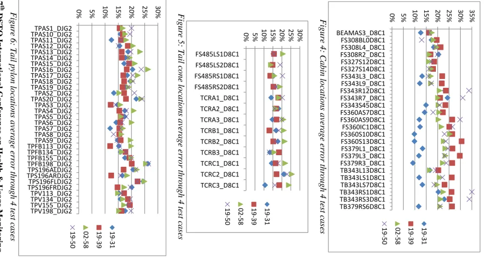
This last data set was included to observe the neural networks’ performance on a manoeuvre significantly different than the one used for training. Table 4 summarizes the performance of the 3 networks on the 4 flight conditions listing the mean squared error, the average percentage error over all outputs recorded in each of the 3 structural groups, and the maximum percentage error recorded among all outputs in each of the 3 structural groups. Note that the percentage error values are based on the maximum manoeuvre range. The plots in Figure 4 to Figure 6 show the average MMR errors for each component location through the 4 test cases.

Table 4: Errors in predicting outputs in the cabin, tail cone, and tail pylon Cabin (25 outputs) Tail Cone (13 outputs) Tail Pylon (32 outputs) Flight Condition MSE Avg Error Max Error MSE Avg Error Max Error MSE Avg Error Max Error Fwd VH 19-31 0.038 15.2% 80.5% 0.038 15.5% 75.1% 0.047 17.3% 90.1% Fwd 0.5VH 19-39 0.081 23.3% 92.4% 0.040 16.1% 74.8% 0.043 16.7% 71.6% Fwd 0.5VH 02-58 0.061 20.1% 77.7% 0.058 19.6% 81.4% 0.056 19.3% 75.4% 30°LT 0.8VH 19-50 0.081 22.5% 92.3% 0.050 17.9% 80.2% 0.054 18.7% 81.8% - MSE is the mean squared error

- Average and maximum error were calculated using maximum manoeuvre range error From the testing of the ANNs on the same flight condition as training, forward level flight at VH (flight run 19-31), all three neural networks predicted the majority of components

reasonably well. The average MMR error for the 25 cabin outputs was 15%, 15% for the 13 tail cone outputs, and 17% for the 32 tail pylon outputs. However, it is important to note that at any point in time the error could be as high as the max errors shown in Table 4. In general, components with higher errors were usually ones whose values were very small or varied through a narrow range. Components with lower errors usually had larger strain values or fluctuated through a wider range.

Overall, the maximum manoeuvre range errors varied from 9% at the location with the lowest average error, FS379R3 in the cabin, to 26% at the location with the greatest average error, TPFB198 in the tail pylon. Time history plots for these two locations during training and testing are shown in Figure 7 and Figure 8. In the first case, the network predicted the signal very well, only under-estimating the lower peaks which was also encountered in training. In the second case, although the average error was higher, the network predicted outputs were still within the correct range of the target signal. Figure 9 shows a magnified plot of cabin location TB379. While the average error for this component was 12%, the predicted signal followed the target output very well with the values in the correct range, the upper peak values closely estimated, the lower peaks sometimes underestimated, and the signal frequency matched well. Figure 10 shows the ANN output for this same load plotted against the target output. Consistent with the time history plot, more values were underestimated than overestimated but the number of outliers was small.

(9)

AIAC14 Fourteenth Australian In

ternational Aerospace Congress

7

th

DSTO Internationa

l Conference on

Health & Usage Monitoring

(HUMS 2011)

Figure 4: C

abin locations average

error through 4 test cases

Figure 5: Tail cone locations a

verage error thro

ugh 4 test cases

Figure 6: Tail pylon locations av

erage error thro

ugh 4 test cases

0% 5% 10% 15% 20% 25% 30% 35% BEAMAS3_D8C1 FS308BL0D8C1 FS308L4_D8C1 FS308R2_D8C1 FS327S12D8C1 FS327S14D8C1 FS343L3_D8C1 FS343L9_D8C1 FS343R12D8C1 FS343R7_D8C1 FS343S45D8C1 FS360AS7D8C1 FS360AS9D8C1 FS360IC1D8C1 FS360S10D8C1 FS360S13D8C1 FS379L1_D8C1 FS379L3_D8C1 FS379R3_D8C1 TB343L13D8C1 TB343LS1D8C1 TB343LS7D8C1 TB343RS1D8C1 TB343RS3D8C1 TB379RS6D8C1 19 ‐ 31 19 ‐ 39 02 ‐ 58 19 ‐ 50 0% 5% 10% 15% 20% 25% 30% FS485LS1D8C1 FS485LS2D8C1 FS485RS1D8C1 FS485RS2D8C1 TCRA1_D8C1 TCRA2_D8C1 TCRA3_D8C1 TCRB1_D8C1 TCRB2_D8C1 TCRB3_D8C1 TCRC1_D8C1 TCRC2_D8C1 TCRC3_D8C1 19 ‐ 31 19 ‐ 39 02 ‐ 58 19 ‐ 50 0% 5% 10% 15% 20% 25% 30% TPAS1_DJG2 TPAS10_DJG2 TPAS11_DJG2 TPAS12_DJG2 TPAS13_DJG2 TPAS14_DJG2 TPAS15_DJG2 TPAS16_DJG2 TPAS17_DJG2 TPAS18_DJG2 TPAS19_DJG2 TPAS2_DJG2 TPAS20_DJG2 TPAS3_DJG2 TPAS4_DJG2 TPAS5_DJG2 TPAS6_DJG2 TPAS7_DJG2 TPAS8_DJG2 TPAS9_DJG2 TPFB113_DJG2 TPFB134_DJG2 TPFB155_DJG2 TPFB198_DJG2 TPS196ALDJG2 TPS196ARDJG2 TPS196FLDJG2 TPS196FRDJG2 TPV113_DJG2 TPV134_DJG2 TPV155_DJG2 TPV198_DJG2 19 ‐ 31 19 ‐ 39 02 ‐ 58 19 ‐ 50

(10)

AIAC14 Fourteenth Australian International Aerospace Congress

This paper has been peer reviewed Figure 7: FS379 in cabin with the best

performance MMR error 9.2%

Figure 8: TPFB198 in tail pylon with the poorest performance MMR error 26.2%

Figure 9: TB379 cabin MMR error 11.7% Figure 10: Predicted output vs target output for TB379 0 2 4 6 8 10 12 14 16 18 −1000 −800 −600 −400 −200 0 200 400 Time (s) Output

Training of Neural Network FS379R3_D8C1 (output 87) − MSNE = 5.57737e−003

predicted training target training 0 1 2 3 4 5 6 7 8 9 10 −1400 −1200 −1000 −800 −600 −400 −200 0 200 Time (s) Output

Testing of Neural Network

FS379R3_D8C1 (output 87) − MSNE = 1.32702e−002 predicted testing target testing 0 2 4 6 8 10 12 14 16 18 −180 −160 −140 −120 −100 −80 −60 Time (s) Output

Training of Neural Network TPFB198_DJG2 (output 38) − MSNE = 3.10977e−002

predicted training target training 0 1 2 3 4 5 6 7 8 9 10 −180 −160 −140 −120 −100 −80 −60 Time (s) Output

Testing of Neural Network

TPFB198_DJG2 (output 38) − MSNE = 1.04171e−001 predicted testing target testing

(11)

AIAC14 Fourteenth Australian International Aerospace Congress

When testing the neural networks on forward level flight at 0.5VH, the errors slightly

increased when compared to those at VH. Even for the location with the greatest error of

30%, the predicted values were within the range of the actual target values.

When the neural networks were tested on a completely different manoeuvre, in this case a steady 30° left turn, only a slight increase in error was observed. The maximum manoeuvre range errors ranged from 13% to 35% over the 3 groups.

For the cabin, shown in Figure 4, the errors were lowest for the first test condition (run 19-31) as one would expect since it was the same flight condition as training. Most components had an error between 9% and 15% with a few falling outside that range up to 25% error. For the second and third test cases, forward level flight at 0.5VH on two different days (runs 19-39

and 02-58), the errors were consistent between the two cases and increased slightly from the baseline test case. For the last test condition, steady left turn (run 19-50), only half a dozen components had greatly increased errors (30-35%) and these outputs had higher errors in the baseline condition as well, while the error for the majority of components stayed at about the same level as for the 0.5VH flight condition.

For the tail cone, shown in Figure 5, almost all components were predicted with about 9-17% error for the forward flight maximum speed condition. Through the other test conditions the errors increased slightly.

For the tail pylon, shown in Figure 6, most components were predicted with about 12-17% error for the forward flight max speed condition. In the tail pylon, the errors maintained approximately the same level through the other test conditions which perhaps suggests that the loads in the tail pylon remain constant for these flight conditions.

Discussion

For each structural group (cabin, tail cone, tail pylon), there were several outputs that could be accurately predicted. There were also several outputs which consistently had high average error (these typically exhibited dynamic behaviour or had positive and negative values). It was noted that the testing errors were several times larger than the training errors in many cases, and this outcome may indicate the occurrence of overfitting of the ANNs and the global minima had not actually been reached. Alternatively, it could be an indication that the training data and the testing data were not statistically consistent, so that the testing data could have fallen outside the scope of the training data. These possibilities will be investigated in the work to follow.

Another limitation of this work was the normalization procedure that was used. The input and output parameters were normalized to the range of the parameters for that data file. Future work will look at using a more general normalization method, such as normalizing to the range of the parameter for the particular flight condition or to the range for the entire usage spectrum.

(12)

AIAC14 Fourteenth Australian International Aerospace Congress

It should be noted that for each of these ANNs there were a large number of outputs. The advantage of this configuration was that the analysis was made more compact instead of having an individual ANN for each output. The drawback was that since the convergence of the network was based on the average of the mean squared error for all the outputs reaching a minimum, the assumption then was that all the outputs would converge at the same time. With individual ANNs they would converge separately and as a result the errors would likely be lower.

The ultimate application for this work is to improve accuracy in the calculation of component retirement times (CRTs) so that they reflect more closely the actual usage of the aircraft. The current calculation method is based on a worst-case scenario for how the aircraft will be used in service. It has not been determined at this time what level of accuracy in predicting the loads is required to cause a significant change in the component retirement time calculation. However it is known that important characteristics of the loads for CRTs include the peak values, mean values, and frequency information. The ANNs used in this work have done reasonably well in those regards.

The results obtained thus far in this work are preliminary but encouraging. Raw data was used as input without any pre-processing. In addition, domain knowledge was not incorporated into the selection of the inputs but the results are nonetheless promising. Much more work in this area is needed and is planned to be undertaken. In particular, a step back will be taken to focus on the pre-modelling stage, that is, more intelligent input selection and an assessment of the predictive variables. Data pre-processing options will be explored including filtering, smoothing and signal modulation. Incorporating time history information as an input to the neural network will be investigated. Different models other than the multi-layer perceptron but still within the realm of machine learning may prove to be better analytical tools for this problem.

Concluding Remarks

In this work, the potential of utilizing multi-layer artificial neural networks (ANNs) to determine helicopter airframe loads at fixed locations from flight state and control system (FSCS) parameters was explored. The appeal of using only FSCS parameters is that the instrumentation required to record these parameters already exists and is active on most helicopters. The ultimate application for this work is to improve accuracy in the calculation of component retirement times (CRTs) so that they reflect more closely the actual usage of the aircraft.

A set of three artificial neural networks were coded in MATLAB to predict 70 previously measured outputs in the cabin, tail cone and tail pylon. The preliminary results presented in this paper show that although the ANNs were not successful for every location, 30 flight state and control system parameters could be used to model these fixed airframe components with reasonable accuracy (approx 15% error) for forward level flight, even when tested on flight manoeuvres at speeds different than the one performed during training. Work is currently being done to validate this assertion for other manoeuvres, and based on testing on a

(13)

AIAC14 Fourteenth Australian International Aerospace Congress

particular manoeuvre, steady left turn at 30 degrees, the results seem hopeful. Certainly there is much work to follow to improve the ANNs, in particular, incorporating pre-modelling and pre-processing techniques. However, the results obtained thus far demonstrate the strong potential for artificial neural networks to reliably estimate airframe loads on rotary-wing aircraft. Collectively, these results could eventually serve to predict dynamic loads on the main and tail rotor by means of different artificial neural networks.

Acknowledgments

This work was funded in part by Defence Research and Development Canada. The data used for this research was provided by Defence Science and Technology Organisation. The expertise and guidance from the Institute for Information Technology at the National Research Council were greatly appreciated.

References

1. Reed, S., Cole, D., “Development of a Parametric Aircraft Fatigue Monitoring System using Artificial Neural Networks”, Proceedings of the 22nd Symposium of the International Committee on Aeronautical Fatigue, Lucerne, Switzerland, Mar 2003.

2. Polanco, F., “Estimation of Structural Component Loads in Helicopters: A Review of Current Methodologies”, DSTO-TN-0239, Dec 1999.

3. Georgia Tech Research Institute, “Joint USAF-ADF S-70A-9 Flight Test Program”, Summary Report, A-6186, May 2001.

4. Cheung, C., Krake, L., “Helicopter Loads Synthesis using a Neural Network”, Proceedings of the 5th DSTO International Conference on Health & Usage Monitoring, Mar 2007.

5. Mitchell, T., Machine Learning, McGraw-Hill, New York, USA, 1997

6. Mirchandani, G., Cao, W., “On Hidden Nodes for Neural Nets”, IEEE Transactions on Circuits and Systems, Vol 36, p 661-664, 1989.