HAL Id: insu-01498483
https://hal-insu.archives-ouvertes.fr/insu-01498483
Submitted on 27 Aug 2020
HAL is a multi-disciplinary open access
archive for the deposit and dissemination of
sci-entific research documents, whether they are
pub-lished or not. The documents may come from
teaching and research institutions in France or
abroad, or from public or private research centers.
L’archive ouverte pluridisciplinaire HAL, est
destinée au dépôt et à la diffusion de documents
scientifiques de niveau recherche, publiés ou non,
émanant des établissements d’enseignement et de
recherche français ou étrangers, des laboratoires
publics ou privés.
LMD-MGCM predictions
Arnaud Stiepen, Sonal Kumar Jain, Nicholas M. Schneider, Justin I. Deighan,
Francesco Gonzalez-Galindo, Jean-Claude Gérard, Zachariah Milby, Michael
H. Stevens, Stephen Bougher, J. Scott Evans, et al.
To cite this version:
Arnaud Stiepen, Sonal Kumar Jain, Nicholas M. Schneider, Justin I. Deighan, Francesco
Gonzalez-Galindo, et al.. Nitric oxide nightglow and Martian mesospheric circulation from MAVEN/IUVS
observations and LMD-MGCM predictions. Journal of Geophysical Research Space Physics, American
Geophysical Union/Wiley, 2017, 122 (5), pp.5782-5797. �10.1002/2016ja023523�. �insu-01498483�
Nitric oxide nightglow and Martian mesospheric circulation
from MAVEN/IUVS observations and LMD-MGCM
predictions
A. Stiepen1 , S. K. Jain2 , N. M. Schneider2 , J. I. Deighan2, F. González-Galindo3 ,
J.-C. Gérard1, Z. Milby2 , M. H. Stevens4 , S. Bougher5 , J. S. Evans6 , A. I. F. Stewart2,
M. S. Chaffin2, M. Crismani2, W. E. McClintock2 , J. T. Clarke7 , G. M. Holsclaw2 ,
F. Montmessin8 , F. Lefèvre8, F. Forget9, D. Y. Lo10 , B. Hubert1, and B. M. Jakosky2
1Laboratoire de Physique Atmosphérique et Planétaire, Space sciences, Technologies and Astrophysics Research (STAR) Institute, University of Liège, Liège, Belgium,2Laboratory for Atmospheric and Space Physics (LASP), University of Colorado Boulder, Boulder, Colorado, USA,3Instituto de Astrofísica de Andalucía, CSIC, Granada, Spain,4Space Science Division, Naval Research Laboratory, Washington, District of Columbia, USA,5Climate and Space Sciences and Engineering Department, University of Michigan, Ann Arbor, Michigan, USA,6Computational Physics, Inc., Springfield, Virginia, USA, 7Center for Space Physics, Boston University, Boston, Massachusetts, USA,8LATMOS/IPSL, Guyancourt, France, 9Laboratoire de Météorologie Dynamique (LMD), Paris, France,10Lunar and Planetary Laboratory, University of Arizona, Tucson, Arizona, USA
Abstract
We report results from a study of nitric oxide nightglow over the northern hemisphere of Mars during winter, the southern hemisphere during fall equinox, and equatorial latitudes during summer in the northern hemisphere based on observations of the𝛿 and 𝛾 bands between 190 and 270 nm by the Imaging UltraViolet Spectrograph (IUVS) on the Mars Atmosphere and Volatile EvolutioN mission (MAVEN) spacecraft. The emission reveals recombination of N and O atoms dissociated on the dayside of Mars and transported to the nightside. We characterize the brightness (from 0.2 to 30 kR) and altitude (from 40 to 115 km) of the NO nightglow layer, as well as its topside scale height (mean of 11 km). We show the possible impact of atmospheric waves forcing longitudinal variability, associated with an increased brightness by a factor of 3 in the 140–200∘ longitude region in the northern hemisphere winter and in the −102∘ to −48∘ longitude region at summer. Such impact to the NO nightglow at Mars was not seen before. Quantitative comparison with calculations of the LMD-MGCM (Laboratoire de Météorologie Dynamique-Mars Global Climate Model) suggests that the model globally reproduces the trends of the NO nightglow emission and its seasonal variation and also indicates large discrepancies (up to a factor 50 fainter in the model) in northern winter at low to middle latitudes. This suggests that the predicted transport is too efficient toward the night winter pole in the thermosphere by ∼20∘ latitude north.1. Introduction
The upper atmosphere of Mars is an intermediate region whose properties (dynamics, structure, and composition) depend on its interactions with the lower atmosphere and the solar activity [Bougher et al., 2015a, 2015b]. The primary goal of NASA Mars Atmosphere and Volatile Evolution (MAVEN) [Jakosky et al., 2013] spacecraft is the study of escape rates and processes for the Martian atmosphere. Detailed analysis of the upper atmosphere of Mars advances our understanding of the coupling of Mars’s atmosphere with solar forcing and its evolution through atmospheric escape. In particular, nitric oxide nightglow is a key tracer of day-to-night hemispheric transport and of the winter polar descending circulation pattern that occurs in the upper atmosphere of Mars.
Nitric oxide UV nightglow comes from deexcitation of NO(C2Π) molecules that result from radiative
recombi-nation. In the dayside thermosphere of Mars, solar extreme ultraviolet radiation photodissociates CO2and N2
molecules. O(3P) and N(4S) ground state atoms are carried by the day-to-night hemispheric transport. They
preferentially descend in the nightside mesosphere (45 to 110 km) in the winter hemisphere. O(3P) and N(4S)
atoms can radiatively recombine to form NO(C2Π). These excited NO molecules directly relax by emitting
pho-tons in the UV𝛿 bands and in the 𝛾 bands through cascades via the A2Σ, v′= 0 state (see equations (1) to (4)).
RESEARCH ARTICLE
10.1002/2016JA023523
Special Section:
Major Results From the MAVEN Mission to Mars
Key Points:
• We study nitric oxide nightglow at equinox, summer, and winter and compare to the LMD-MGCM predictions
• This study reveals the seasonal control on the emission, as well as unexpected longitudinal variations caused by waves/tides
• We suggest future work on NO nightglow using GCMs and IUVS disk images and tangent limb data
Correspondence to:
A. Stiepen,
arnaud.stiepen@ulg.ac.be
Citation:
Stiepen, A., et al. (2017), Nitric oxide nightglow and Martian mesospheric circulation from MAVEN/IUVS observations and LMD-MGCM predictions, J. Geophys. Res.
Space Physics, 122, 5782–5797,
doi:10.1002/2016JA023523.
Received 26 SEP 2016 Accepted 24 MAR 2017
Accepted article online 29 MAR 2017 Published online 31 MAY 2017 Corrected 31 MAY 2017
This article was corrected on 31 MAY 2017. See the end of the full text for details.
©2017. American Geophysical Union. All Rights Reserved.
These emissions are thus indicators of the N and O atom fluxes transported by the dayside to nightside and the winter descending circulation pattern from the nightside thermosphere to the mesosphere.
N(4S) + O(3P)→ NO(C2Π) (1)
NO(C2Π)→ NO(X2Π) +𝛿 bands (2)
NO(C2Π)→ NO(A2Σ, v′= 0) + 1.22 μm (3)
NO(A2Σ, v′= 0)→ NO(X2Π) +𝛾 bands (4)
Bertaux et al. [2005] reported the first detection of the NO UV nightglow at Mars. The Spectroscopy for Inves-tigation of Characteristics of the Atmosphere of Mars (SPICAM) [Bertaux et al., 2006] spectrograph on board ESA-Mars Express (MEX) observed NO nightglow in two modes: tangent limb and stellar occultation. Bertaux et al. [2005] observed an emission peak reaching 2.2 kR at an altitude of ∼70 km during limb observations. Due to the relative abundance of O over N in the nightside mesosphere, the limiting factor for this emission is the nitrogen atom flux descending toward the atmospheric layer where N atoms recombine with O to pro-duce NO in the excited C2Π state. They estimated a downward flux of 2.5 × 10⁸N atoms cm−2s−1, about one
third of the estimated production of N atoms by EUV photodissociation of N2molecules on the dayside. Subsequently, using 21 limb observations performed by SPICAM, Cox et al. [2008] provided a detailed analysis of the correlations between the emission peak brightness and altitude and latitude, local time, the interplane-tary magnetic field, and solar activity. They noticed the large variability of the NO nightglow, with no apparent correlation among these factors. They found that the vertical emission profiles peaked at 1.2 ± 1.5 kR and the nightglow layer peak was located at 73 ± 8 km.
Gagné et al. [2013] used 2215 SPICAM stellar occultation observations, in which NO nightglow was detectable in 128. They reported an interannual variability of the number of detections of the emission, with more detections found at higher solar activity, in agreement with the paradigm of production of N(4S) by
photodis-sociation of N2on the dayside. They found that the peak altitude ranges from 40 to 130 km, with a mean value
of 83 ± 24 km, and an associated brightness of 4 ± 3.5 kR. They compared their observations to the Global Climate Model (GCM) for Mars developed at the Laboratoire de Météorologie Dynamique (LMD-MGCM) described by González-Galindo et al. [2009] and Lopez-Valverde et al. [2011a, 2011b]. They showed that the model predicts brighter NO nightglow during winter at polar latitudes than elsewhere and shows little latitude dependence during equinoxes, with the exception of polar latitudes. While overall reasonable agreement between the SPICAM and model peak intensities was found, some striking differences were identified. Dur-ing the northern winter, SPICAM observed intense emissions in the low-latitude regions, not predicted by the model. On the other hand, strong emissions were predicted by the model in the winter polar region at this season, while SPICAM did not observe particularly strong emissions there. During the equinox season, the model predicted strong emissions in both polar regions, while SPICAM was only able to detect emissions in the high latitudes in a few occasions.
Stiepen et al. [2015] compiled 10 years of stellar occultation and limb observations of the NO𝛿 and 𝛾 bands performed by SPICAM (5000 observations, out of which more than 200 present NO emissions) to study the variability of the summer-to-winter hemispherical circulation in the upper atmosphere of Mars. Their data set fully included and extended the ones used by Cox et al. [2008] and Gagné et al. [2013]. Stiepen et al. [2015] provided a statistical study of the vertical emission profile, which peaked at 5 ± 4.5 kR and was situated at 72 ± 10.4 km. Its brightness and altitude ranged from 0.23 to 18.5 kR and from 42 to 97 km, respectively. They showed that the number of detections increases at higher solar activity, yet the peak characteristics (brightness and altitude) remain unchanged for different solar activity levels, an unexpected result. Using the complete SPICAM NO database, they constructed maps of the brightness of the nitric oxide nightglow at different seasons. These maps showed large data gaps in the summer hemisphere and at polar latitudes, especially in the north (see their Figure 3). In comparison with the (Mars Atmosphere and Volatile EvolutioN Mission-Imaging UltraViolet Spectrograph) MAVEN-IUVS observations, the amount of SPICAM data is lower and covers different years and solar activity.
SPICAM observations and the LMD-MGCM model comparisons raise important questions that require fur-ther investigation. The variability of the NO𝛿 and 𝛾 bands indicates variability in the hemispheric circulation.
Knowledge of the morphology of the NO𝛿 and 𝛾 bands on Venus [e.g., Feldman et al., 1979; Stewart and Barth, 1979; Stewart et al., 1980; Bougher et al., 1990; Bougher and Borucki, 1994; Gérard et al., 1981, 2008; Stiepen et al., 2012, 2013] brought relevant information constraining the circulation of Venus’s upper atmosphere. At Venus, the NO nightglow layer peaks at 115 km ± 2 km [Gérard et al., 1981; Stiepen et al., 2012], within Venus’ thermo-sphere. At Mars, N atoms cross two different atmospheric regions (the thermosphere and the mesosphere) and then recombine with O atoms to produce NO(C2Π) molecules. Furthermore, the circulation patterns followed
by N atoms at Venus (subsolar to antisolar circulation) and Mars (summer dayside to winter nightside hemi-sphere in the thermohemi-sphere) are different. These important differences suggest that Martian NO nightglow is regulated by a circulation pattern that spans the dayside thermosphere (the peak of the dayside N production is ∼140 km), and the nightside thermosphere and mesosphere (as low as 40 km [Stiepen et al., 2015]). N atoms thus cross a ∼100 km vertical section of the Martian atmosphere, thereby following a complicated circulation pattern with different regimes between the mesosphere and the thermosphere.
Bertaux et al. [2005] explained that because the abundance of O atoms is much larger than N atoms, N down-ward flux is the limiting factor for the NO emission. Differences in peak brightness and altitude are thus indicators of variations of the delivery of N atoms to the nightside mesosphere. Considering Venus, Stiepen et al. [2012] used a one-dimensional chemical-diffusive model to simultaneously model the globally averaged NO and O2(a1Δg) airglow vertical distributions using CO2and O density profiles based on the Visible and Infrared Thermal Imaging Spectrometer (VIRTIS) and Spectroscopy for Investigation of Characteristics of the Atmosphere of Venus (SPICAV) observations. They conducted a sensitivity study of the eddy diffusion coeffi-cient and N downward flux at high altitude in the nightside and showed that the eddy coefficoeffi-cient influences both the NO nightglow peak altitude and brightness. They also show that the downward nitrogen flux only acts on the peak intensity at Venus. Bougher and Borucki [1994] also tested the impact of the variable eddy diffusion (Kz) on the nightside of Venus. They showed that a factor of 5 variation of the Kzhas a large impact
on the resulting N and O density profiles and the associated nightglow layers (see their Figure 14). Brecht et al. [2011] performed a numerical Venus study that suggested that the altitude location of the nightglow is con-trolled by both eddy diffusion and vertical winds, while the NO intensity is mainly concon-trolled by the vertical winds (see their Tables 3 and 4).
The current study uses periapse limb scans of the ultraviolet nightside of Mars obtained by the Imaging UltraViolet Spectrograph (IUVS) instrument on board the MAVEN spacecraft to provide a detailed analysis of the NO nightglow spectrum. We provide insights on the hemispherical thermospheric circulation through the NO nightglow emission in northern winter, around southern fall equinox, and close to the equator during northern summer. Based on the LMD-MGCM study by Gagné et al. [2013], the downward N and O fluxes are most important during winter, in contrast with summer, while equinoxes are transition periods during which the latitude is thought to play only a minor role in the NO nightglow distribution, with the exception of the polar regions. However, this prediction has not been confirmed by NO observations, so far. SPICAM limb and stellar occultations data provide, at best, one NO nightglow vertical profile for every orbit of Mars Express (i.e., 6 h). In this study, we use the IUVS capability to scan the atmosphere up to 12 times during the MAVEN peri-apse phase (22 min) to analyze the short-term (both spatial and temporal) variability of the NO nightglow and its drivers. This capability to provide high cadence data is crucial to characterize the aforementioned variabil-ity of the altitude and brightness of the NO nightglow to provide insight on the influence of the circulation in driving the spatial/seasonal characters of Mars NO nightglow.
2. Observation Geometry, Data Reduction, and Model Description
2.1. MAVEN and IUVS Geometry During NO Nightglow Observations
The MAVEN spacecraft carries one remote sensing instrument for the study of Mars’s upper atmosphere, the Imaging UltraViolet Spectrograph (IUVS) [McClintock et al., 2015]. IUVS has two channels: far-UV (110–180 nm) and mid-UV (180–340 nm) and is mounted on an Articulated Payload Platform (APP) that can orient its field of view relative to Mars. During the MAVEN orbit periapse phase, the APP orients IUVS to look to the side of spacecraft motion, allowing IUVS to use its scan mirror to repeatedly map out the vertical structure of the atmosphere. During the apoapse portion (∼6000 km above the surface) of the MAVEN orbit, IUVS uses its scan mirror to produce an image of the planet. The apoapse images of the NO nightglow will be analyzed in a future study.
The IUVS spectral resolution during limb scans is ∼0.6 nm [McClintock et al., 2015]. IUVS uses a long and narrow slit (10∘ × 0.06∘) placed in the focal plane of the telescope as an entrance to the spectrograph, which defines the instrument field of view. During limb scans, the long axis of the slit is approximately parallel to the limb. IUVS scans the nightside atmosphere between 40 and 250 km altitude, with a vertical resolution of 5 km. The slit image at the detector is divided into seven spatial bins along slit, each associated with its own tangent altitude depending on slit location and orientation. The scan data are altitude-binned to create a single ver-tical profile. Each periapse phase of the orbit provides up to 12 verver-tical scans (and thus 12 verver-tical emission profiles) taken during a 22 min time period in northern winter and up to 24 vertical emission profiles around southern fall equinox due to a change in the observing sequence, resulting in a coarser vertical resolution (10 km). During all observation periods, data were collected following the same latitude—local time track, i.e., predawn data are statistically taken at higher latitudes. At summer, morning data are statistically taken preferentially in the southern hemisphere at higher latitudes.
2.2. Spectral Analysis
Nightglow emissions at Mars have low signal compared to dayglow emissions. To minimize the error intro-duced by dark current and its subtraction, we used a reference superdark image created by coadding multiple dark images of the same binning and exposure in the relevant time period. The local superdark was then scaled by a multiplier and a constant to match the dark current for each orbit of the observations.
Nightside spectra consist primarily of emissions from nitric oxide, though solar spectra can contaminate the spectrum near the terminator, and auroral emissions can occur anywhere during an auroral event [e.g., Schneider et al., 2015, Figure 1]. To isolate the NO emission brightness, we used multilinear regression technique (MLR) to fit the observed spectrum [Stevens et al., 2015]. We used four fit vectors: CO Cameron band, CO+
2 ultraviolet doublet, NO, and a solar spectrum (only used near terminator). For CO Cameron and CO + 2
Ultraviolet doublet bands we used model spectra convolved with line spread function of the instrument [Stevens et al., 2015]. For the solar and nitric oxide templates we used coadded spectra measured by IUVS during disk and nightside observations, respectively. Spectra obtained over different spectral ranges were corrected for missing emission by scale factors derived from the template.
The IUVS was calibrated using UV-bright stars observations, scaled by instrument geometric factors appropri-ate for extended source observations. Intensities presented in this study are linearly dependent on the abso-lute calibration. The intensity values are affected by 30% systematic wavelength-independent uncertainty due to the calibration uncertainties.
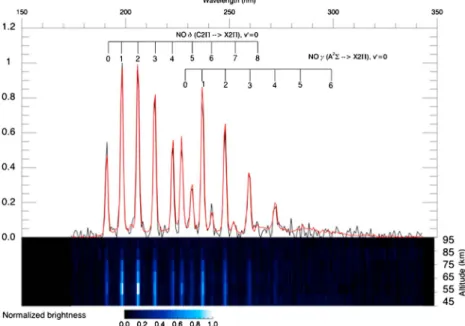
Figure 1 shows the normalized average of 84 spectra of the nitric oxide nightglow recorded by IUVS during MAVEN orbit 387 (10 December 2014, Ls= 250, first scan) (black) and the NO spectrum (red) used in the MLR fit process (top image), and a normalized spectrogram composed of these spectra presented versus altitude from 45 km (bottom) to 95 km (top). The NO spectrum in the MLR was constructed by averaging more than 10 min of IUVS observations during MAVEN orbit 387. In the following sections, we integrated over the wavelength range of the NO𝛿 and 𝛾 bands to characterize the NO nightglow emission in kiloRayleighs (kR).
2.3. Data Coverage
We use limb scans observations by IUVS during the periapse part of MAVEN’s orbit. The northern winter obser-vations were taken from MAVEN orbit 335 (1 December 2014, Ls= 240) to orbit 850 (8 March 2015, Ls= 300),
the southern fall equinox observations were taken from MAVEN orbit 1548 (16 July 2015, Ls= 13) to orbit 1744
(21 August 2015, Ls= 31), and summer data were taken from orbit 2300 (5 December 2015, Ls= 75) to orbit
2799 (8 March 2016, Ls= 115). The seasonal-latitudinal coverage is shown in Figure 2. The detection threshold
of the NO bands is ∼0.1 kR. Out of 592 orbits, this database contains 3586 vertical profiles of the NO night-glow. In addition to an automatic verification procedure (chi-square), the presence of the NO bands is visually verified for each profile, as well as the quality of the MLR fit.
First, we note that detections were made at all nightside solar zenith angles and local times. Cox et al. [2008] showed that local time does not significantly influence the emission on a restricted data set. Gagné et al. [2013], however, indicated (see their Figure 7) that the LMD-MGCM predicts local time influence on both the NO nightglow peak altitude and brightness for equatorial conditions at 180∘< Ls< 210∘. This result could not
be confirmed nor rejected by SPICAM observations, due to a lack of adequate coverage. Unfortunately, our data set also lacks the needed coverage to identify a possible effect of local time on the peak brightness and altitude. We restricted the data set to spectra taken at SZA higher than 110∘, in order to avoid solar radiance
Figure 1. Nitric oxide nightglow observed by IUVS. Normalized average of the NO spectra recorded by IUVS during
MAVEN orbit 387 (10 December 2014,Ls= 250) between 40 and 100 km (black) and MLR fit of the spectrum (red). The bottom image shows the data before fitting by the MLR. Spectra are arranged according to altitude from (top) 95 km to (bottom) 45 km. A weak solar component is visible for wavelengths larger than 270 nm at∼40–50 km. The MLR technique provides a good fit of the NO signal by subtracting this component in the cleaned data, as shown by the quality of the fit.
contamination. We note an increase of the emission toward morning hours; however, morning data are pref-erentially obtained at higher latitudes where the NO brightness increases. As the latitudinal impact on NO nightglow emission is expected to be more important than the local time effect on the emission [Gagné et al., 2013], we focus here on the latitudinal dependence for the emission.
Figure 2 shows the coverage of IUVS NO nightglow detections (white circles) superimposed on the LMD-MGCM prediction for limb brightness at LT = 21 (see section 4 for a discussion on the model
Figure 2. Locations of the NO observations by IUVS (white circles)
superimposed to the LMD-MGCM brightness intensity prediction at LT=21. IUVS observations cover middle to high latitudes in winter (northern hemisphere) and during fall equinox (southern hemisphere) and equatorial latitudes during summer in the northern hemisphere. NO nightglow was detected during all orbits with night limb observation geometry.
configuration and results). Figure 2 shows that the IUVS data set has three advantages compared to SPICAM [see Stiepen et al., 2015, Figure 2]: (i) it extends the observation cover-age toward the northern pole during winter and toward the southern pole around southern fall equinox, (ii) it provides unprecedented cov-erage and data density, including in regions previously observed by SPICAM [Stiepen et al., 2015], and (iii) it concentrates observations obtained under similar solar activity, while the SPICAM data were accumulated dur-ing 10 years of observations coverdur-ing large variations of the solar EUV flux along the 11 year cycle.
During the observations used in this study, solar activity was mod-erate in the descending phase of cycle number 24. We also note that
Schneider et al. [2015] reported an intense period of solar activity (energetic electron precipitation) from 17 December 2014 (MAVEN orbit 435) to 23 December 2014 (MAVEN orbit 453). We focus on short-term variability driven by latitude and solar longitude (i.e., we look for seasonal effects on the NO nightglow) and possible local changes (i.e., with longitude). We provide quantitative comparisons of the nitric oxide night-glow altitude, brightness, and scale height and the LMD-MGCM calculated values in the three seasons. The IUVS coverage will allow to revisit and provide additional insights into the data-model differences identified in Gagné et al. [2013]. In particular, the northern winter region and the equinox in the southern hemisphere are now much better covered, so the increase of emission toward the pole predicted by the model can be confirmed or rejected on the basis of this extended observational data set.
3. Observational Results
3.1. Mapping the NO Nightglow Layer
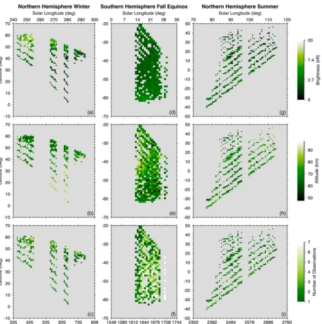
The detected limb brightness on individual profiles ranges from 0.16 kR to 12 kR in southern fall equinox, from 0.21 kR to 47 kR at the northern winter hemisphere, and from 0.15 to 20 kR close to the equator during summer in the southern hemisphere (see Table 1). The highest values thus exceed those observed by Stiepen et al. [2015] (from 0.2 to 18.5 kR). This difference is explained by the different coverage: IUVS data span closer to the northern winter pole. The lower values depend on the sensitivity to the emission of each instrument. Figure 3 shows solar longitude (Ls) maps of the NO nightglow intensity and altitude. We determine the
alti-tude, brightness, and location (latitude and Ls) of the peak of each observed profile of the NO nightglow. We
then display the average value within each 1∘ Ls/1∘ latitude bin of the peak brightness or altitude and the number of observations in each bin. Figures 3 have a different color scale than the LMD-MGCM map shown in Figure 2 to better display small-scale variations of the brightness. Overall, Figure 3 shows that the NO night-glow layer is brighter and at lower altitude in the atmosphere toward the pole in southern fall equinox and northern winter. This would confirm the behavior predicted by the LMD-MGCM and is an interesting differ-ence with respect to SPICAM results. A more detailed comparison with the LMD-MGCM results is presented in section 4. Note that both IUVs data and the simulations presented in this study share a vertical resolution of 5 km.
Figures 3a–3c show the peak brightness, peak altitude, and number of observations of the NO nightglow in each bin in northern winter, respectively. Figures 3d–3f show the same quantities at southern fall equinox and Figures 3g–3i show the same quantities during northern summer.
During northern winter, we observe NO nightglow brightness ranging from 0.21 kR to 47 kR. As we show averages in Figure 3, brightness in individual profiles may exceed the given values. The extreme and mean values for each season are provided in Table 1. The average peak altitude ranges from 47 to 107 km, with the layer lower in the atmosphere toward the pole. The number of observations in each bin depends on the geometrical constraints of IUVS and MAVEN along its orbit and does not reflect physical processes. During fall equinox, the NO nightglow brightness ranges from 0.16 kR to 12 kR. The peak altitude varies between 42 and 118 km, with a decrease of the altitude toward the pole, with very few exceptions. We also observe a variability of the peak altitude up to 45 km difference within two adjacent bins, suggesting extreme variability in the local dynamics of the mesosphere in the nightside. During northern summer, NO nightglow brightness ranges from 0.15 kR to 20 kR. The peak altitude ranges from 42 to 118 km.
Figure 3 and Table 1 show a large variability of the brightness during winter, up to almost 2o orders of mag-nitude. The longitudinal variability of the brightness of the NO nightglow emission will be analyzed in the next section. The properties of the emission differ from winter to equinox and summer. First, the latitudinal gradient of the emission altitude and brightness is less striking for equinox and summer conditions. Second, the variability of the peak brightness at midlatitudes in southern fall equinox is less than in northern winter (also, see Figure 7). Finally, the scale height is constant in southern fall equinox toward the pole and in equa-torial latitudes during summer in the northern hemisphere, while it decreases from 10 to 8 km in northern winter. The mean topside scale height of the emission was calculated by fitting each vertical profile topside part by an exponential function using a Levenberg-Marquardt method. The average scale height for northern winter, fall equinox, and northern summer are 9, 13, and 10 km, respectively. We note that the scale height derived from this data set is higher than that reported by Cox et al. [2008]: from 3.8 to 11.0 km, with a mean value of 6 ± 1.7 km.
Table 1. IUVS Data
Northern Winter Fall Equinox Northern Summer
Intensity (kR) Altitude (km) Intensity Altitude Intensity Altitude
Mean 4.7 70 1.9 71 1.7 70
1𝜎 5.2 8 1 10 1.6 9
Minimum 0.21 40 0.16 42 0.15 42.5
Maximum 47 107 12 118 20 117
Figure 3. Seasonal mapping of the NO nightglow. All Figures have 1∘latitude per 1∘solar longitude bins. Shown are the (a) average limb brightness of the emission peak, (b) the altitude of the emission layer, and (c) the number of observations in each bin, all color coded at winter. (d–f ) and (g–i) The same quantities as Figures 1a–1c but at fall equinox and summer in the northern hemisphere, respectively. The number of observations in each bin is dependent on observation geometry and does not reflect physical processes.
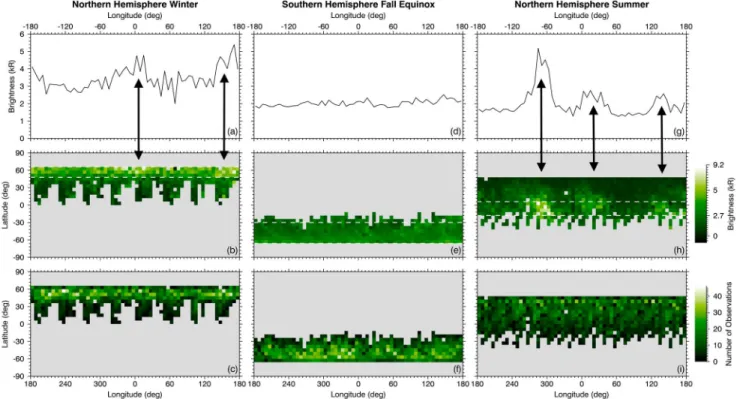
Figure 4. Geographical mapping of the NO nightglow. All maps have 1∘latitude per 1∘longitude bins. Shown are (a) the average limb brightness of the emission peak versus longitude, (b) the average brightness of the peak, and (c) the number of observations in each bin for winter in the northern hemisphere conditions. (d–f ) and (g–i) The same quantities as in Figures 4a–4c but at fall equinox and during summer in the northern hemisphere, respectively.
We used the technique described in Hubert et al. [2016] to retrieve volume emission rates (VER) of the emis-sion. VERs presented in this study will be used in a future study to quantitatively compare radiances from limb observations and disk images obtained by the IUVS instrument. We note that, during northern winter, VERs range from ∼15 to ∼150 photons cm−3s−1at the peak from the equator to the pole, thus an order of
magnitude higher at the winter pole. In fall equinox, the VER rate increases by a factor of ∼4 from the equa-tor to polar latitudes, ranging from 10 to 40 photons cm−3s−1. At northern summer, it ranges from 9 to 80
photons cm−3s−1, almost covering 1 order of magnitude. 3.2. Longitudinal Control of the NO Airglow Layer
Figure 3 shows the longitudinal and latitudinal variations of the NO emission. The emission is generally brighter at higher latitudes. Unexpected brightenings of the emission are observed in certain longitude sec-tors. This longitudinal analysis could not be performed by earlier studies and is now possible thanks to IUVS data higher density. The NO nightglow layer is brighter in one region at midlatitudes in the northern hemi-sphere during winter. The brightest emission is found between 140∘ and 200∘ longitude and is more intense by a factor ∼2 when compared to the mean brightness observed in this season. To a lesser extent, brightening can be seen in Figure 4a between −40∘ and 20∘ longitude. We calculated a paired Student’s t test between the average emission in these regions that indicates that the hypothesis that the 120∘ to 180∘ longitude region is statistically different from the other longitude regions is verified at the 99% confidence level. In contrast, the data suggest that no longitude region shows enhanced NO nightglow emission during fall equinox in the southern hemisphere. During northern summer, Figure 4i shows the most intense brightening of NO night-glow that occurs in the −102∘ to −48∘ longitude, between −5∘ and 55∘ and between 120∘ and 180∘ longitude regions close to the equator. In the −102∘ to −48∘ longitude region, the brightening of NO nightglow reach a factor as high as ∼3 when compared to the mean brightness observed in the data during that season. The unexpected structure during northern summer, with prominent wave 3 structure and a bright peak at geographic longitudes −102∘ to −48∘ during summer, merited closer examination. A possible explanation for the longitudinal control on NO nightglow is that the emission is enhanced in some longitude sectors by a combination of waves. The midlatitudes of the winter northern hemisphere are known to be significantly
Figure 5. Vertical profiles of the NO nightglow recorded by IUVS during
MAVEN orbit 588 (Ls= 255, winter in the northern hemisphere). The box indicates the latitude of the peak of each vertical emission profile, which is shown by the black arrows. Profiles observed at higher-latitude peak lower in the atmosphere and are brighter.
affected by large-scale planetary waves, including standing and trav-eling waves [e.g., Banfield et al., 2004; Hinson and Wang, 2010; Lewis et al., 2016; Medvedev et al., 2011]. Longi-tudinally dependent thermal tide activity has also been reported in the upper atmosphere of Mars during the northern hemisphere fall/winter sea-son [Keating et al., 1998; Wilsea-son, 2002; Lo et al., 2015; England et al., 2016]. The LMD-MGCM simulations suggest an effect on NO nightglow that migrates over local time with a dominant period of about 2 sols, suggesting traveling planetary waves [e.g., Forbes et al., 2002; Withers et al., 2003; Bougher et al., 2004]. We subdivided the data into quarters by time to test whether the brightness might be attributed to some transient phenomenon limited in time or might evolve in geographic longitude structure. The longitude pattern was consistent between the four quarters within the limit of noise in the data. We therefore find that the peaks are persistent in time and not due to temporal transients. Further-more, the lack of dependence on local time argues against a tidal explana-tion, as a shift of 6 h (each orbit with 12 complete scans covered about 2 h going forward in time about 30 min, then back 2 h; the data coverage for the whole season begins at 05:00 and ends at 22:00) would be expected to shift the longitude maxima in 90∘ in longitude for a diurnal tide. For the wave 3 structure detected, the longitudes of maximum emission at a given local time should correspond to minimum emission about 4 h later. We are therefore left with the conclusion that the longitudinal structure in nightglow is relatively fixed with geographic longitude at northern summer and must indicate some way in which circulation patterns are controlled by the underlying topography. We note that the brightest peak overlies the Tharsis bulge and Valles Marineris, but further analysis is not warranted until modeling is better able to reproduce the low altitudes of the emission.
3.3. Short Timescale Latitudinal Variability of the Emission During Winter
As the IUVS data set provides an unprecedented coverage of the NO nightglow closer to the winter northern pole, we focus on the latitudinal variations of the peak brightness and altitude during northern winter. We first analyze the correlation between the latitude and the peak brightness for the 12 vertical emission profiles IUVS takes during one sample orbit (Figure 5). The peak altitude, brightness and latitude are extracted from the multiple limb profiles to study their variations during the 22 min of the periapse phase. Within one orbit, we focus on the latitudinal variation of the nightglow layer. Figure 5 shows vertical profiles of the NO nightglow observed during orbit 588 (Ls = 255∘). The five-limb profiles showed in Figure 5 were measured at different
latitudes during the same orbit. Therefore, the changes in both altitude and brightness of the peak reflect the latitudinal control on the emission. We note that the profiles observed at higher latitude peak lower in the atmosphere and are brighter (ranging from 1 kR at 77 km at 50∘N to 9 kR at 59 km at 58∘N). These profiles were obtained at constant solar longitude and within less than 20 min. The altitude of the peak decreases from 77 km to 58 km toward the northern winter pole, thus, about two NO nightglow emission scale heights.
Figure 6. Time series of the NO brightness at the peak in northern winter
from 40 to 50∘N latitude. Data are presented by the black squares. Circles show the mean value in each 1∘ LSbin and vertical bars represent the 1𝜎 variability around the mean values in each bin. The period during which the SEP and IUVS instruments reported an intense precipitation of energetic electrons associated with diffuse aurora in Mars’s atmosphere is indicated in grey. The increase of brightness in not related with a quasi-simultaneous electron precipitation event.
This suggests large differences in N downward flux to the nightside meso-sphere as the brightness of the NO nightglow increases by 1 order of magnitude within 10∘ latitude toward the winter pole.
For each orbit, we calculate the lin-ear correlation coefficient of the peak brightness and altitude, on the one hand, and the latitude of the peak of the emission, on the other hand. Linear Pearson correlation coefficient values range from 0.56 (i.e., low control of the brightness with the latitude for this orbit) to 0.97 (i.e., high control of the brightness with the latitude in this orbit), with a mean value of 0.83 (i.e., mean of all coefficients, one per orbit). We note that all the coefficients are positive, indicating that the bright-ness of the peak increases toward polar latitudes. At fall equinox and northern summer, we found a nega-tive correlation coefficient (the peak altitude decreases toward higher latitudes), ranging from −0.2 to −0.96, with a mean value of −0.5. The latitudinal control on the emission is thus less striking under these conditions. The negative values indicate that the emission is brighter toward the south pole at fall equinox and northern summer.
3.4. Temporal Evolution of the Emission During Winter
We also examine the seasonal variation of the emission to determine the possible impact of energetic electron precipitation in Mars’s atmosphere on the NO nightglow emission. Photoelectron impact on N2is known to
be a significant source of dissociation and production of N(4S) atoms in Mars’s and Venus’s atmospheres. This
was demonstrated in a study of N atom production on the Venus dayside by Gérard et al. [1988] who showed that electron collisions with N2contribute significantly to the N atom production in the thermosphere. This source was included in the Venus Thermospheric General Circulation Model (VTGCM) [see Bougher et al., 1990; Brecht et al., 2011], and considered as an important source of N atoms on Mars ([Fox, 1993]). Schneider et al. [2015] reported an intense period of energetic electron precipitation in Mars’s atmosphere, associated with the detection of UV diffuse aurora on Mars’s nightside, from 17 December 2014 (orbit 435) to 23 December 2014 (orbit 453).
Figure 6 shows the brightness of the emission at northern midlatitudes (between 40∘ and 50∘ latitude) during winter (black squares). Circles show the mean value in each 1∘ LSbin, and vertical bars represent the standard deviation around the mean values in each bin. The brightness increases from Ls= 245∘ (orbit 385) to Ls= 252∘
(orbit 430), followed by a plateau from Ls = 252∘ (orbit 430) to Ls= 258∘ (orbit 453), followed by a decrease
from Ls = 258 (orbit 453) until Ls = 300 (orbit 735), when winter is coming to an end. This variation is not
predicted by the LMD-MGCM. The brightness of NO nightglow thus increased before the SEP event reported by Schneider et al. [2015], which is indicated in the figure by a grey zone. Furthermore, at lower latitudes (from equatorial to 40∘), the increase is absent from this time series. This suggests that the variability of the NO nightglow brightness is caused by the intrinsic seasonal variability and not driven by external processes such as electron precipitation.
4. Comparisons to the LMD-MGCM
We have used in this work the Global Climate Model (GCM) for Mars developed at the Laboratoire de Météorologie Dynamique (LMD-MGCM). This global model is able to simulate the thermal and dynamical state
of the Martian atmosphere, as well as its composition, from the surface to the exobase [González-Galindo et al., 2009]. A detailed description of the parameterizations included in the LMD-MGCM can be found in Forget et al. [1999], Montmessin et al. [2004], Lefèvre et al. [2004], and in Angelats i Coll et al. [2005] and González-Galindo et al. [2005, 2009] for the relevant processes in the upper atmosphere. Most important for this work, the LMD-MGCM includes a photochemical model of the upper atmosphere (both neutral and ions), able to simu-late the emission of NO nightglow by tracing the recombination of N and O atoms [Gagné et al., 2013]. More details about the photochemical model can be found in González-Galindo et al. [2011, 2013]. Note that in the standard version of the LMD-MGCM this photochemical model is only used at altitudes above the 0.1 Pa level (about 70 km). However, given that this altitude corresponds approximately to the observed peak altitude of the NO emission, in the simulations used here the upper atmosphere chemistry is extended downward up to the 10 Pa level. It is also important to note here that the current version of the photochemical model does not include the dissociation of neutral species by photoelectrons, including N2, which has been shown to be
a significant source of odd nitrogen at Venus [Bougher et al., 1990].
The simulation shown here was run using the latest available version of the LMD-MGCM, described in González-Galindo et al. [2015], and used to build the version 5.2 of the Mars Climate Database [Millour et al., 2016]. There are a number of differences with the model used in a previous comparison with Mars Express data [Gagné et al., 2013]. These include the radiative effect of water ice clouds, known to have a significant effect over the mesospheric temperatures [Navarro et al., 2014], an improved version of the non-LTE radia-tive transfer [Lopez-Valverde et al., 2014] and a dynamical core allowing for parallelization. The simulation covers a full Martian year simulation and uses a solar flux appropriate for solar average conditions and a cli-matology scenario for the dust load, representative of a standard Mars year without any global dust storm [Millour et al., 2016].
Now we provide a qualitative comparison of the observed NO nightglow brightness and altitude with the prediction of the LMD-MGCM. This will allow us to suggest future improvements to the model. We test two GCM predictions versus the IUVS observations:
1. The emission is predicted to be brighter at the winter pole, and the emission peak altitude is expected to be lower at higher latitudes. In southern fall equinox, the emission is not expected to be controlled by latitude for low and midlatitude conditions (from ∼70∘N to 60∘S at Ls∼ 0∘).
2. The latitudinal control of the NO nightglow in southern fall equinox is predicted to be similar to the one in northern winter: brighter and lower in the atmosphere toward the poles [see Gagné et al., 2013, Figures 5, 6a, and 6d; and Figure 2 here). The LMD-MGCM model predicts longitudinal variability of the emission caused by waves. These predictions need observational confirmation.
We also analyze the possibility for an impact of solar flares on the NO nightglow emission and provide sug-gestions for future studies using tangent limb and disk images obtained during the apoapse phase of the spacecraft orbit and GCMs.
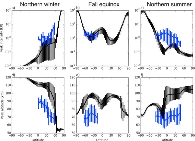
By comparing Tables 1 and 2, we note that the model underestimates the NO nightglow intensity by a mean factor of ∼10 in northern winter, predicts the brightness accurately during fall equinox, and is ∼8.5 too low at equatorial latitudes during summer in the northern hemisphere. The discrepancies are beyond the sys-tematic uncertainties of the IUVS absolute calibration (∼30%). We note also that the LMD-MGCM predicts NO nightglow brightness as low as 0.01 kR that cannot be observed as it is below IUVS threshold of detection. The intensity and altitude comparison are best illustrated in Figure 7, where we compare IUVS observations to the LMD-MGCM. The shown model results are 30∘ Ls averages (Ls = 240∘ –270∘ for northern winter,
Ls= 0∘ –30∘ for fall equinox, and Ls= 90∘ –120∘ for northern summer) during nighttime hours. Blue and black
lines show the average data and model values in 5∘ and 3.75∘ latitude bins, respectively. Vertical bars show the 1𝜎 deviation around the mean values. Figures 7a–7c show the brightness of the peak of the emission and Figures 7d–7f show its altitude versus latitude during northern winter, fall equinox, and northern summer, respectively.
We note that the LMD-MGCM correctly reproduces to first order the latitudinal variability of the peak emission and peak altitude during northern winter and fall equinox, but not during northern summer. The model also predicts the emission scale height well: average of 10, 11, and 10 km at northern winter, fall equinox, and northern summer, respectively. This is in agreement with the IUVS data within less than 20%. In addition,
Table 2. LMD
Northern Winter Fall Equinox Northern Summer
Intensity (kR) Altitude (km) Intensity Altitude Intensity Altitude
Mean 0.5 101 1.7 95 0.3 95
1𝜎 1.1 20 1.4 8 0.4 11
Minimum 0.01 48 0.2 54 0.02 60
Maximum 13.6 124 13.6 110 6 112
there are significant differences in the mean values between the model and the observations at all seasons, with a predicted emission peak generally much weaker and higher in the atmosphere than observed. During northern winter (Figures 7a and 7d) the model underestimates the brightness of the NO nightglow by a factor up to 50 in the low latitudes, and between about 4 and 15 in the middle to high latitudes. An important increase of brightness is predicted by the model at latitudes higher than 60∘N, while IUVS observations show an increase of emission from about 30∘N. Note that the observed behavior differs from that inferred from SPICAM observations. At this season, maximum emission was observed by SPICAM around 30∘N, with many negative detections around 60∘N [Gagné et al., 2013; Stiepen et al., 2015], while IUVS data clearly show intensity increasing with increasing latitude. Regarding the peak altitude, while both model and data show a general decrease when approaching the winter pole, the predicted peak is about 30 km higher than observed. During fall equinox (see Figures 7c and 7d), the LMD-MGCM correctly predicts the brightness of the emis-sion. Both model and data show a modest latitudinal variation, with brightness increasing toward the pole, although the increase is steeper in the model than in the data. Note that this is again a difference with respect to SPICAM previous observations, which did not show strong emissions in the poles during equinox. Regarding the peak altitude, it is again overestimated by about 20 km.
Figure 7. Comparison between IUVS data and the LMD-MGCM calculations. Black and blue lines show the average data and model values in the 1∘latitude bin, respectively. Vertical bars show the 1𝜎deviation around the mean values. Shown are the brightness of the peak of the emission and its altitude versus latitude during (a, d) northern winter, (b, e) fall equinox, and (c, f ) northern summer.
During northern summer (see Figures 7e and 7f ), the peak intensity is again underestimated, with differences up to a factor of 10. Note also that the model predicts a strong increase of the emission with increasing latitude in the southern hemisphere, not seen in the data. Regarding the peak altitudes, the model predicts a strong decrease of the peak altitude when going from the northern to the southern hemisphere, which is neither confirmed by the observations. As in the other seasons, overall, the peak altitudes are significantly higher in the model than in the observations.
5. Discussion
The important data-model differences at all the studied seasons clearly suggest that there are significant deficiencies in the treatment of the chemical and dynamical processes considered in the GCM.
One possibility to explain the underestimation of the peak intensity during northern winter and summer is that the LMD-MGCM transports N atoms too efficiently toward the winter poles, producing a strong concen-tration of N in the polar regions and a depletion in the low and middle latitudes. We note that the model predicts very strong emissions in the polar regions, where observations are lacking. We also note that Clancy et al. [2013] found, by comparing 1.27 μm O2airglow observations from MRO-CRISM and LMD-MGCM pre-dictions, that the model overestimates the transport of oxygen toward the poles by 25%, in agreement with our results.
Another possibility is that the model underestimates the formation of N in the dayside. As mentioned above, the formation of N atoms by photoelectron impact dissociation of N2, known to be important on Venus, is not
considered in the model. Also, a precise computation of the N2photodissociation requires the use of very high
spectral resolution, usually not achievable by GCMs. However, this underestimation in N production would in principle affect all seasons, while the model predicts correctly the observed brightness at the southern fall equinox. A more conclusive answer would require observations at all latitudes and an integration over the whole planet.
The strong overestimation of the peak altitude suggest that the model is not correctly representing the ver-tical O and/or N density profiles. A possibility is that the temperatures predicted by the model are too high in the mesosphere, producing a N and O peak too high in the atmosphere. However, comparisons with Mars Climate Sounder data, although they indicate some model deficiencies in the polar regions, do not show a warm bias in the modeled mesosphere [Forget et al., 2014]. It is also possible that the chemistry conducing to the production and destruction of N and O atoms is not adequately represented in the model.
The unexpected longitudinal variability of the NO nightglow brightness suggests the importance of dynami-cal impact of waves on the emission. We note that the observed variations cannot be caused by tides, as they are observed at all nightside local times and during a large period of time. Impact of geographic structure on the nightside mesosphere was not observed before using the NO nightglow as a tracer of propagating waves in this region of Mars’s atmosphere. A full analysis of these waves cannot be performed on the basis of this data set. It would require distinguishing between local time and longitude effects which are not well distin-guished in the existing data set. In order to expand this research, the complementary analysis of LMD-MGCM, MGITM-GCM, and IUVS observations of Mars’s disks revealing NO nightglow will address the question of the impact of waves on the NO nightglow emission.
6. Conclusions and Future Work
We selected nitric oxide nightglow vertical profiles obtained by the IUVS instrument on board the MAVEN spacecraft to conduct an analysis of the variability of the NO𝛿 and 𝛾 bands in the winter northern hemi-sphere, the southern hemisphere during fall equinox, and equatorial latitudes during summer in the northern hemisphere.
For these conditions, under moderate solar activity, we showed that the NO nightglow exhibits important variations in brightness and altitude with latitude, solar longitude and geographic longitude. This indicates changes in the N flux, in addition to changes in the O density profile in the nightside mesosphere during the time and location this data set was obtained. We compared our results to LMD-MGCM predictions for the brightness and altitude of the peak, as well as the topside scale height of the NO nightglow vertical pro-file. The model correctly represents the emission in southern fall equinox, but in contrast during northern
winter and summer, the observed brightness are higher by a factor between about 4 and 50 than predicted. The peak altitudes are systematically overestimated by the model in about 20 km.
Comparison of the three seasons suggests that the model dynamics transports N atoms to the nightside thermosphere at higher (polar) latitudes than observed toward the winter pole and reproduces correctly the dynamics in southern fall equinox. We however cannot rule out the possibility that the model underpredicts the production of N on the dayside, as it would require data at all latitudes during one season.
We provided the first analysis of multiple scans during a short timescale (less than an hour) and found that profiles from different latitudes during one periapse phase of the MAVEN orbit have brighter peaks lower in the atmosphere for high latitudes, a result similar to the statistical study we also provided.
We showed the possible impact of planetary traveling waves on Mars’s nightside mesosphere by quantifica-tion of the longitudinal control on the NO nightglow emission. Data show longitudinal structures (brightening of the emission) that are persistent during the night and during the observation period. This suggests that Mars’s nightside mesosphere was impacted during the period of observations by a combination of planetary waves. A detailed analysis of that hypothesis is beyond the scope of this study and is an interesting topic for future work.
These recent NO nightglow measurements from the Mars Atmosphere and Volatile EvolutioN Mission-Imaging UltraViolet Spectrograph (MAVEN/IUVS) will next be compared to Mars Global Ionosphere-Thermosphere Model (M-GITM) simulations. The M-GITM model is described in great detail in Bougher et al. [2015a, 2015b]. Its odd nitrogen chemistry will be updated according to that presented in Brecht et al. [2011], thereby enabling the model to simulate self-consistently the chemistry and dynamics of NO nightglow for-mation above ∼40 km. In addition, the production of dayside N(4S) atoms will include a source by electron
impact, based on the VTGCM at Venus and motivated by the comparison presented in this study. The strong data-model differences clearly show that an in-depth revision of the implementation in the LMD-MGCM of the chemical and dynamical processes at the origin of N and O production, destruction, and transport is needed. In particular, the effects of photoelectrons, important for N production on Venus, is currently being implemented in the GCM. A revision of the current implementation of the N2photodissociation, including comparisons with high-resolution calculations, will also be performed. The photochemical scheme will also be reviewed; the effects of uncertainties in chemical reaction rates will be assessed and possible missing reactions will be incorporated if needed. A more precise and faster photochemical core is currently being implemented at the LMD, which may also affect the results shown here. This new photochemical core will be used in the future to unify the two different photochemical schemes used for the lower and the upper atmosphere.
Other pending questions, such as the morphology of the emission and the local time control of the emission, will be analyzed in a future study by using nadir images of the NO nightglow obtained by IUVS/MAVEN. Improved understanding of the N and O density distributions can also be obtained by comparing simultane-ous observations of the NO UV nightglow from IUVS and the O2IR emission with SPICAM-IR on board Mars
Express and the CRISM instrument on board the Mars Reconnaissance Orbiter. These concurrent measure-ments of airglow at two atmospheric levels involving two species with different lifetimes would provide strong constraints on the transport from the dayside to the nightside.
We now can combine to the specific observation goals inherited from SPICAM studies a higher density of IUVS data that allows in-depth comparison to GCMs. Our understanding of Mars’s upper atmosphere complex circulation patterns will benefit from these improvements.
References
Angelats i Coll, M., F. Forget, M. A. Lopez-Valverde, and F. González-Galindo (2005), The first Mars thermospheric general circulation model: The Martian atmosphere from the ground to 240 km, Geophys. Res. Lett., 32, L04201, doi:10.1029/2004GL021368.
Banfield, D., B. J. Conrath, P. J. Gierash, R. J. Wilson, and M. D. Smith (2004), Traveling waves in the Martian atmosphere from MGS TES Nadir data, Icarus, 170, 365–403.
Bertaux, J.-L., et al. (2005), Nightglow in the upper atmosphere of Mars and implications for atmospheric transport, Science, 307, 566–569. Bertaux, J.-L., et al. (2006), SPICAM on Mars Express: Observing modes and overview of UV spectrometer data and scientific results,
J. Geophys. Res., 111, E10S90, doi:10.1029/2006JE002690.
Bougher, S. W., J. C. Gérard, A. I. F. Stewart, and C. G. Fesen (1990), The Venus nitric oxide night airglow: Model calculations based on the Venus thermospheric general circulation model, J. Geophys. Res., 95, 6271–6284.
Acknowledgments
A. Stiepen is supported by the Fund for Scientific Research (F.R.S.-FNRS). The MAVEN mission is supported by NASA through the Mars Exploration Program in association with the University of Colorado and NASA’s Goddard Space Flight Center. M. Stevens is supported by the NASA MAVEN Participating Scientist program. B. Hubert and J.-C. Gerard acknowledge support from the SCOOP/BRAIN program of the Belgian Federal Government. A. Stiepen also thanks M. Dumont for her help in the finalization of the figures. F.G.-G. is funded by the European Union Horizon 2020 Programme (H2020 Compet-08-2014) under grant agreement UPWARDS-633127. The LMD-MGCM results used in this paper are available under request to F.G.-G. (ggalindo@iaa.es). IUVS level 1B data used in this study are archived in the Planetary Data System. They are labeled v07r01 periapse.
Bougher, S. W., and W. J. Borucki (1994), Venus O2visible and IR nightglow: Implications for lower thermosphere dynamics and chemistry,
J. Geophys. Res., 99, 3759–3776.
Bougher, S. W., S. Engel, D. P. Hinson, and J. R. Murphy (2004), MGS Radio Science electron density profiles: Interannual variability and implications for the Martian neutral atmosphere, J. Geophys. Res., 109, E03010, doi:10.1029/2003JE002154.
Bougher, S. W., T. E. Cravens, J. Grebowksy, and J. Luhmann (2015a), The aeronomy of Mars: Characterization by MAVEN of the upper atmosphere reservoir that regulates volatile escape, Space Sci. Rev., 195, 423–456, doi:10.1007/s11214-014-0053-7.
Bougher, S. W., D. Pawlowski, J. M. Bell, S. Nelli, T. McDunn, J. R. Murphy, M. Chizek, and A. Ridley (2015b), Mars Global
Ionosphere-Thermosphere Model: Solar cycle, seasonal, and diurnal variations of the Mars upper atmosphere, J. Geophys. Res. Planets,
120(2), 311–342.
Brecht, A. S., S. W. Bougher, J.-C. Gérard, C. D. Parkinson, S. Rafkin, and B. Foster (2011), Understanding the variability of nightside temperatures, NO UV and O2IR nightglow emissions in the Venus upper atmosphere, J. Geophys. Res., 116, E08004, doi:10.1029/2010JE003770.
Clancy, T., et al. (2013), Correction to ‘Extensive MRO CRISM observations of 1.27μm O2airglow in Mars polar night and their comparison to MRO MCS temperature profiles and LMD GCM simulations’, J. Geophys. Res. Planets, 118, 1148–1154, doi:10.1029/2011JE004018. Cox, C., A. Saglam, J.-C. Gérard, J.-L. Bertaux, F. González-Galindo, F. Leblanc, and A. Reberac (2008), Distribution of the ultraviolet nitric
oxide Martian airglow: Observations from Mars Express and comparisons with a one-dimensional model, J. Geophys. Res, 113, E08012, doi:10.1029/2007JE003037.
England, S. L., et al. (2016), Simultaneous observations of atmospheric tides from combined in situ and remote observations at Mars from the MAVEN spacecraft, J. Geophys. Res. Planets, 121, 594–607, doi:10.1002/2016JE004997.
Feldman, P. D., H. W. Moos, J. T. Clarke, and A. L. Lane (1979), Identification of the UV nightglow from Venus, Nature, 279, 221–222. Forbes, J., et al. (2002), Nonmigrating tides in the thermosphere of Mars, J. Geophys. Res., 107, 5113, doi:10.1029/2001JE001582. Forget, F., F. Hourdin, R. Fournier, C. Hourdin, O. Talagrand, M. Collins, S. R. Lewis, P. L. Read, and J.-P. Huot (1999), Improved general
circulation models of the Martian atmosphere from the surface to above 80 km, J. Geophys. Res., 104, 24,155–24,175.
Forget, F., et al. (2014), Simulating the Mars Climate with the LMD Mars Global Climate Model: validation and issues, The Fifth International
Workshop on the Mars Atmosphere: Modelling and Observation, edited by F. Forget and M. Millour, Oxford, U. K.
Fox, J. L. (1993), The production and escape of nitrogen atoms on Mars, J. Geophys. Res., 98, 3297–3310.
Gagné, M.-E., J.-L. Bertaux, F. González-Galindo, S. Melo, F. Montmessin, and K. Strong (2013), New nitric oxide (NO) nightglow measurements with SPICAM/MExas a tracer of Mars upper atmosphere circulation and comparison with LMD-MGCM model prediction: Evidence for asymmetric hemispheres, J. Geophys. Res. Planets, 118, 2172–2179, doi:10.1002/jgre.20165.
Gérard, J.-C., A. I. F. Stewart, and S. W. Bougher (1981), The altitude distribution of the Venus ultraviolet nightglow and implications on vertical transport, Geophys. Res. Lett., 8, 633–636.
Gérard, J. C., E. J. Deneye, and M. Lerho (1988), Sources and distribution of odd nitrogen in the Venus daytime thermosphere, Icarus, 75(1), 171–184.
Gérard, J.-C., C. Cox, A. Saglam, J. L. Bertaux, E. Villard, and C. Nehmé (2008), Limb observations of the ultraviolet nitric oxide nightglow with SPICAV on board Venus Express, J. Geophys. Res., 113, E00B03, doi:10.1029/2008JE003078.
González-Galindo, F., M. A. Lopez-Valverde, M. Angelats i Coll, and F. Forget (2005), Extension of a Martian general circulation model to thermospheric altitudes: UV heating and photochemical models, J. Geophys. Res., 110, E09008, doi:10.1029/2004JE002312. González-Galindo, F., F. Forget, M. A. Lopez-Valverde, M. Angelats I Coll, and E. Millour (2009), A ground-to-exosphere Martian general
circulation model: 1. Seasonal, diurnal and solar cycle variations of thermospheric temperature, J. Geophys. Res., 114, E04001, doi:10.1029/2008JE003246.
González-Galindo, F., A. Maatanen, F. Forget, and A. Spiga (2011), The Martian mesosphere as revealed by CO2cloud observations and
general circulation modeling, Icarus, 216, 10–22, doi:10.1016/j.icarus.2011.08.006.
González-Galindo, F., J.-Y. Chaufray, M. A. Lopez-Valverde, G. Gilli, F. Forget, F. Leblanc, R. Modolo, S. Hess, and M. Yagi (2013), Three-dimensional Martian ionosphere model: 1. The photochemical ionosphere below 180 km, J. Geophys. Res. Planets, 118, 2105–2123, doi:10.1002/jgre.20150.
González-Galindo, F., M. A. Lopez-Valverde, F. Forget, M. García-Comas, E. Millour, and L. Montabone (2015), Variability of the Martian thermosphere during eight Martian years as simulated by a ground-to-exosphere global circulation model, J. Geophys. Res. Planets, 120, 2020–2035, doi:10.1002/2015JE004925.
Hinson, D. P., and H. Wang (2010), Further observations of regional dust storms and baroclinic eddies in the northern hemisphere of Mars,
Icarus, 206, 290–305.
Hubert, B., C. Opitom, D. Hutsemékers, E. Jehin, G. Munhoven, J. Manfroid, D. V. Bisikalo, and V. I. Shematovich (2016), An inversion method for cometary atmospheres, Icarus, 277, 237–256, doi:10.1016/j.icarus.2016.04.044.
Jakosky, B., et al. (2013), Mars atmosphere and volatile evolution (MAVEN) mission to Mars, Space Sci. Rev., 195(1–4), 3–48, doi:10.1007/s11214-015-0139-x.
Keating, G. M., et al. (1998), The structure of the upper atmosphere of Mars: In situ accelerometer measurements from Mars Global Surveyou, Science, 279, 1672–1676.
Lefèvre, S., S. Lebonnois, F. Montmessin, and F. Forget (2004), Three-dimensional modeling of ozone on Mars, J. Geophys. Res., 109, E07004, doi:10.1029/2004JE002268.
Lewis, S. R., D. P. Mulholland, P. L. Read, L. Montabone, R. J. Wilson, and M. D. Smith (2016), The solsticial pause on Mars: 1. A planetary wave reanalysis, Icarus, 264, 456–464.
Lo, D. Y., et al. (2015), Nonmigrating tides in the Martian atmosphere as observed by MAVEN IUVS, Geophys. Res. Lett., 42(21), 9057–9063. Lopez-Valverde, M. A., G. Sinnabend, M. Sornig, and P. Kroetz (2011a), Modelling the atmospheric CO210μm non-thermal emission in Mars
and Venus at high spectral resolution, Planet. Space Sci., 59(10), 999–1009, doi:10.1016/j.pss.2010.11.011.
Lopez-Valverde, M. A., F. González-Galindo, and M. Lopez-Puertas (2011b), Revisiting the radiative balance of the mesosphere of Mars,
The Fourth International Workshop on the Mars Atmosphere: Modelling and Observation, edited by F. Forget and E. Millour, pp. 359–362,
Paris, France.
Medvedev, A. S., E. Ygit, P. Hartogh, and E. Becker (2011), Influence of gravity waves on the Martian atmosphere: General circulation modeling, J. Geophys. Res., 116, E10004, doi:10.1029/2011JE003848.
McClintock, W. E., et al. (2015), The Imaging Ultraviolet Spectrograph (IUVS) for the MAVEN mission, Space Sci. Rev., 195(1–4), 75–124, doi:10.1007/s11214-014-0098-7.
Millour, E., et al. (2016), Exploring the Interannual Variability of the Martian Atmosphere with the Mars Climate Database v5.2, Abstract from the 41st COSPAR Scientific Assembly that was to be held 30 July–7 August at Istanbul Congress Center (ICC), Turkey, but was cancelled.
Montmessin, F., F. Forget, P. Rannou, M. Cabane, and R. M. Haberle (2004), Origin and role of water ice clouds in the Martian water cycle as inferred from a general circulation model, J. Geophys. Res., 109, E10004, doi:10.1029/2004JE002284.
Navarro, T., J.-B. Madeleine, F. Forget, A. Spiga, E. Millour, F. Montmessin, and A. Maattanen (2014), Global climate modeling of the Martian water cycle with improved microphysics and radiatively active water ice clouds, J. Geophys. Res. Planets, 119, 1479–1495, doi:10.1002/2013JE004550.
Schneider, N., et al. (2015), Discovery of diffuse aurora on Mars, Science, 350, 6261, doi:10.1126/science.aad0313.
Stevens, M. H., et al. (2015), N2in the upper atmosphere of Mars observed by IUVS on MAVEN, Geophys. Res. Lett, 42, 9050–9056. Stewart, A. I., and C. A. Barth (1979), Ultraviolet night airglow of Venus, Science, 205, 59–62.
Stewart, A. I. F., J. C. Gérard, D. W. Rusch, and S. W. Bougher (1980), Morphology of the Venus ultraviolet night airglow, J. Geophys. Res., 85, 7861–7870.
Stiepen, A., L. Soret, J.-C. Gérard, C. Cox, and J.-L. Bertaux (2012), The vertical distribution of the Venus NO nightglow: Limb profiles inversion and one-dimensional modeling, Icarus, 220, 981–989.
Stiepen, A., J.-C. Gérard, M. Dumont, C. Cox, and J.-L. Bertaux (2013), Venus nitric oxide nightglow mapping from SPICAV nadir observations,
Icarus, 226, 428–436.
Stiepen, A., J. Gérard, M. Gagné, F. Montmessin, and J.-L. Bertaux (2015), Ten years of Martian nitric oxide nightglow observations, Geophys.
Res. Lett., 42, 720–725, doi:10.1002/2014GL062300.
Wilson, R. J. (2002), Evidence for nonmigrating thermal tides in the Mars upper atmosphere from the Mars Global Surveyor Accelerometer Experiment, Geophys. Res. Lett., 29, 1120, doi:10.1029/2001GL013975.
Withers, P., S. W. Bougher, and G. M. Keating (2003), The effects of topographically-controlled thermal tides in the Martian upper atmosphere as seen by the MGS accelerometer, Icarus, 164(1), 14–32.
Erratum
The authorship byline has been corrected to reflect additional contributions by M. Crismani. The present version may be considered the authoritative version of record.